Environmental Regulations and Competitiveness:Evidence based on Chinese firm data∗

Ankai Xu†

(Preliminary Draft)

Abstract

This paper provides empirical evidence in support of the Porter hypothesis that

tighter environmental regulations can increase productivity under certain circum-

stances. It builds on a theoretical model in which environmental regulations induce

firms to adopt more efficient technologies. Using Chinese firm-level data covering

a ten-year period, the empirical study examines the effects of two specific policy

instruments - the pollution levy and regulatory standards - on firm productivity. It

finds a bell-shaped relationship between water pollution levies and the total factor

productivity of firms, indicating that an increase in the pollution levy rate can be

associated with higher productivity. In addition, the study investigates the effect of

pollution emission standards on firm productivity and identifies an initial negative

effect which diminishes after a period of three years.

Keywords: Environmental regulations, Innovation, Productivity, Porter hypothesis, China

JEL Classifications: D2, F18, Q52, Q55, Q56

∗The opinions expressed in this paper should be attributed to its author. They are not meant torepresent the positions or opinions of the WTO and its Members and are without prejudice to Members’rights and obligations under the WTO.†Graduate Institute of International and Development Studies. Email: ankai.xu@graduateinstitute.ch.

1 Introduction

The effects of environmental regulations on the competitive performance of industries have

been the subject of heated debate since the start of the environmental movement in the

early 1970s. Two opposing arguments are at the heart of this debate. On the one hand,

opponents of stricter environmental regulations argue companies tend to locate their busi-

ness activities in countries or regions where environmental regulations are relatively lax,

resulting in so-called “pollution havens”. On the other hand, Porter and Van der Linde

(1995) argue that the costs of compliance with environmental regulations will be offset by

cost reductions resulting from technological innovation stimulated by these regulations.

This argument is also known as the “Porter hypothesis”. According to Porter, an increase

in environmental standards can actually improve competitiveness, offset compliance costs

and encourage firms to upgrade to new and cleaner technologies.

Empirical analysis on the economic cost of environmental regulations can be traced back

to the 1970s, and most studies were conducted in the United States. Jaffe et al. (1995)

provides a review of the literature. Notably, Levinson (1996) examines the effect of state

environmental regulations of varying stringency on the location choice of firms, and shows

that interstate differences in environmental regulations do not systematically affect the

location choices of most manufacturing plants. Becker (2011) measures the effects of en-

vironmental regulations on plant-level productivity in all U.S. manufacturing industries

employing spatial-temporal variations in environmental compliance costs. The results

suggest that, for the average plant, there is no statistically significant effect on produc-

tivity. Greenstone et al. (2012) used detailed production data from 1.2 million U.S. plant

observations drawn from the 1972-1993 Annual Survey of Manufacturers, and conclude

that among surviving polluting plants, stricter air quality regulations are associated with

a roughly 2.6 percent decline in total factor productivity (TFP).

Since Porter and Van der Linde (1995) introduced the concept that properly designed en-

vironmental standards can trigger innovation and induce technological change, a growing

literature has looked at the positive effects of innovation. See Ambec et al. (2013) for an

overview of the theory and empirical evidence on the Porter hypothesis. Most empirical

research focuses on the relationship between regulations and innovation, and the evidence

remains inconclusive. For example, Jaffe and Palmer (1997) find that lagged environ-

mental compliance expenditures have a significant positive effect on R&D expenditures.

Berman and Bui (2001) show increases in productivity among oil refineries in the United

States, despite heavy compliance costs in response to local air pollution regulations. Stud-

ies focusing on environmentally related patents find a positive relationship between the

number of successful green patents with environmental regulations (Johnstone et al., 2010;

1

Popp, 2006; Lanoie et al., 2011).

This study employs a rich Chinese firm-level dataset to evaluate the effects of Chinese envi-

ronmental regulations on productivity of firms. As a rapidly-growing developing country,

China provides a unique context to study the effects of environmental regulations. In the

last three decades, China’s remarkable economic growth dwarfed many other economies,

but it has also brought serious environmental degradation. In recent years, recognizing

the danger of environmental degradation and the increasing popular demand for better

environmental quality, the Chinese government has implemented various pollution control

policies.

A few studies in the literature investigate the impacts of environmental regulations and

industrial pollution controls in China. For example, Jiang et al. (2014) examine firm-

level emission data and find that both foreign-owned firms and domestic publicly-listed

firms show less intensive pollutant emissions compared to state-owned enterprises (SOEs).

The study also finds that larger firms, firms in industries that export more, and firms

with more educated employees pollute less; and that better property rights protection is

negatively correlated with pollutant discharges over and beyond the national standards.

Jefferson et al. (2013) exploit the plausibly exogenous variation in regulatory stringency

generated by the Two Control Zone policy in China to find evidence that environmental

regulations induce pollution-intensive firms to improve economic performance, whereas

energy-intensive firms suffer from negative externalities of the regulations.

The current paper is one of the first studies to systematically look at the effect of different

pollution control regulations on firm productivity. Environmental regulations may affect

productivity at the firm-level in at least two ways. First, compliance with environmental

regulations may require firms to divert inputs - capital, labor, material inputs, etc. -

towards the production of environmental quality, resulting in lower productivity. Second,

regulations may necessitate changes in the production process and induce firms to adopt

more efficient, cleaner technologies. This study presents evidence in favour of a more

recent approach which views environmental policy as a positive force leading to increased

productivity and enhanced competitiveness.

The analysis builds on a theoretical model where tighter environmental regulations in-

duce firms to upgrade production technologies, resulting in both pollution reduction and

productivity increase under certain conditions. The empirical analysis examines two par-

ticular policy instruments - the pollution levy (or pollutant tax) and pollution emission

standards - and their effects on the total factor productivity (TFP) of firms. It finds evi-

dence in support of the Porter hypothesis. With regards to the pollution levy, it discovers

a non-linear correlation between the effective water levy and firm productivity, suggest-

2

ing that a pollution levy does not necessarily harm productivity; on the contrary, higher

pollution levy could induce firms to upgrade to cleaner technologies and at the same time

increase productivity. In particular, the study identifies a threshold of the pollution levy

where a higher levy rate corresponds to higher productivity. The paper also investigates

the effects of industry-specific pollution emission standards on productivity and finds that,

although the introduction of a pollution emission standard can lead to an initial drop in

productivity, the negative effect diminishes over a period of three years.

The findings in this paper are different from similar studies conducted in industrialized

countries, where a negative correlation is often observed between environmental regu-

lations and productivity. The discovery of a non-linear relationship between pollution

control measures and productivity in China is of important policy relevance. Compared

with industrialized countries which find themselves at the efficient production frontier,

firms in a developing country like China tend to rely on low production technologies, and

are therefore more likely to switch to cleaner and more efficient technologies in response to

stringent environmental regulations, resulting in both productivity increases and emission

reductions. The findings in the study can also be potentially relevant in other developing

countries going through a rapid economic transition.

The remainder of the paper proceeds as follows. Section 2 gives a brief introduction of

China’s environmental regulations. Section 3 presents a simple model where environ-

mental regulations in the form of a pollution levy and emission standards lead to higher

productivity. Section 4 introduces the data. Section 5 specifies the empirical strategy and

reports the results. Section 6 concludes.

2 Institutional background1

China’s legal and institutional development of environmental protection goes back to the

1970s. The Environmental Protection Law (EPL), which was first enacted in 1979 on

a provisional basis and which formally came into effect in 1989, is the main legal basis

for environmental management in China. The EPL lays out general principles for envi-

ronmental protection and describes key instruments for environmental management. It

requires enterprises to assess the environmental impacts of proposed projects and comply

with all relevant environmental standards. This statute also clarifies which environmental

regulations should be managed and enforced at national level, and which ones at local

1Summary based on OECD (2006), Environmental Compliance and Enforcement in China: An As-sessment of Current Practices and Ways Forward (Draft study presented at the second meeting of theAsian Environmental Compliance and Enforcement Network, 4-5 December 2006, in Hanoi, Vietnam).http://www.oecd.org/environment/outreach/37867511.pdf

3

level. In addition, the EPL recognizes the rights of organizations and individuals to report

cases of pollution and file charges against polluters.

In 1988, the State Environmental Protection Agency (SEPA) was formed alongside nu-

merous local Environmental Protection Bureaus (EPBs) throughout the nation. In 2008,

SEPA was replaced by the Ministry of Environmental Protection (MEP). Over the past

30 years, many environmental protection organizations other than the EPBs have also

been formed at both the national and local (provincial, city, or county) levels. Accord-

ing to the data released by MEP, China had established 12,215 environmental protection

institutions by the end of 2008, with 393 at the national and provincial levels.2

Due to the different levels of economic development across different regions in China,

local governments and authorities are encouraged to institute local rules and regulations

that are adapted to local circumstances - as long as they do not conflict with those at

the national level. By 2009, China had established or passed one environmental protec-

tion law, 26 individual environmental laws, over 50 administrative regulations concerning

environmental protection and over 1600 local environmental decrees and rules.

There are a number of regulatory and economic instruments dealing with industrial pol-

lution control in China. The most important ones include (1) the Pollution Levy System,

(2) Emission/discharge and environmental quality standards, (3) the Discharge Permit

System, and (4) Shutting down, merging and transferring of existing polluting plants. In

addition, newly-constructed industrial plants have to conduct an Environmental Impact

Assessment and integrate pollution treatment into the design, construction and operation

of a new plant (the so-called “Three Simultaneities” requirement). Below I briefly de-

scribe the two most commonly used policy instruments - the Pollution Levy System and

Emission/Discharge Standards.

2.1 Pollution Levy System

China’s pollution levy system was first introduced as a legal provision in the Water Pollu-

tion Prevention and Control Law of 1984. Subsequently, regulations such as the Interim

Measures for Pollution Levy were established to stipulate the implementation of the sys-

tem. In 2003, the Administrative Regulations on Pollution Discharge Levy were enacted

by the State Council, which marked a major shift in the system.

Originally, pollution that exceeded emission/discharge standards were subject to a fine.

Since the introduction of the new pollution regulation in 2003, the calculation of the

pollution levy is no longer based on the amount of pollution exceeding the standards, but

2China Environment Yearbook, 2009 (in Chinese)

4

on the total amount of emissions generated by the firm. The formula used for calculating

the levy incorporates both the volume of total wastewater/air discharge and the degree to

which each pollutant concentration exceeds the standard. The polluter is required to pay

levies on the sum of the highest three pollutant-specific levies rather than for a cumulative

amount of all pollutant emissions. A detailed description of the pollution levy system in

China can be found in Appendix B.

Although the formulas to calculate the pollution levy is determined by the national

pollution levy regulation, in practice, the levy rate varies substantially across different

provinces. There are four major sources of variations in provincial pollution levy rates.

First, concentration standards of hazardous pollutants are set jointly by the national and

local governments and can vary by region. Second, the pollution levy standards differ by

pollutant. According to China’s pollution levy regulations, the actual levy is the greatest

of all potential levies for each pollutant discharged by a plant before 2003, and the sum

of the three highest potential levies calculated for each pollutant after 2003, differences

in the composition of pollutants in pollution emissions could lead to different levy rates.

Third, there are significant differences in enforcement capacity at the local level. Stud-

ies indicate that more frequent inspections by local EPBs can lead to higher reported

pollution and thus higher pollution levies (Lin, 2013). Finally, the levy can be reduced

or even eliminated at the discretion of local regulators after inspections. Such leeway

introduces considerable variation into regional enforcement practices of the pollution levy

system.

Until recently, the revenue collected from the pollution levy was used to cover the oper-

ating expenses of environmental authorities. Currently, the revenue is directed towards

environmental protection measures and the purchasing of monitoring equipment. Of the

total pollution levy revenues, 10% is transferred to the central government and 90% re-

mains at the sub-national level.

2.2 Environmental Standards

The 1989 Environmental Protection Law authorized SEPA to establish two types of na-

tional standards: environmental quality (ambient) standards and pollution emission stan-

dards. Ambient standards designate the maximum allowable concentrations of pollutants

in the atmosphere. Emission standards, on the other hand, designate the maximum al-

lowable concentrations of pollutants in industrial pollution emissions. Local governments

may create ambient and emission standards for pollutants not specified in the national

standards, and they may also establish stricter upper limits for pollutants compared to

those set by the national standards. The pollution emission/discharge standards provide

5

a basis for the EPB inspection activities.

China issued the first ambient environmental quality standard for surface water in 1983.

The standard was subsequently updated in 1988, 1999 and 2002. In addition, the first

Integrated Wastewater Discharge Standard was issued in 1988 and updated in 1998. The

wastewater discharge standard establishes the upper limits for 69 pollutant concentrations

and the allowable water discharges for some industries. In addition, a range of water dis-

charge and emission standards target specific industries including chemicals, coal mining

and processing, electroplating, iron and steel, municipal wastewater treatment, pharma-

ceuticals, pesticides, pulp and paper, etc.

Ambient air quality has been regulated in China since 1982, when initial limits were set

for TSP (Total Suspended Particulates), SO2, NO2, lead, and BaP (Benzo(a)pyrene).

In 1996, the standard was both strengthened and expanded under the new National

Ambient Air Quality Standard. In February 2012, China released a new ambient air

quality standard, GB 3095-2012, which sets limits for the first time on PM2.5. The new

standards will take full effect nationwide in 2016, but many cities and regions in China

are required to implement the standards earlier than the national timeline. China also

issued a range of air pollution emission standards targeting specific industries and sectors,

such as cement, ceramics, coal, minerals, thermal power industries, etc., at the national

and provincial level.

Appendix C lists the national and provincial pollution emission standards published since

1996.

3 A model of regulation and productivity

In this section, I describe a simple general equilibrium model where innovation may al-

leviate or even completely offset the costs of environmental regulations (Mohr, 2002).

I then discuss two environmental policy instruments - the pollution levy and technical

regulations - and their effect on productivity.

Assume an economy with perfect information and a constant population consisting of N

agents. The market is perfectly competitive. To begin with, all producers in the economy

use the same technology. Later I extend the model to allow for the possibility of an

additional new technology.

Each agent is endowed with li unit of labor per period of time. Aggregated labor supply

is L =∑N

i=1 li. The agent devotes this labor to the production of a single consumption

good ci. The output of ci depends on the input of li and a cumulative capital ki specific

6

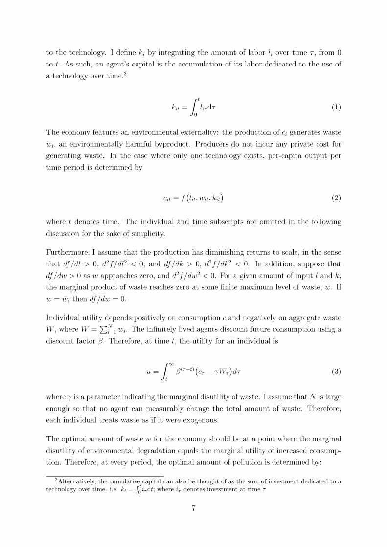
to the technology. I define ki by integrating the amount of labor li over time τ , from 0

to t. As such, an agent’s capital is the accumulation of its labor dedicated to the use of

a technology over time.3

kit =

∫ t

0

liτdτ (1)

The economy features an environmental externality: the production of ci generates waste

wi, an environmentally harmful byproduct. Producers do not incur any private cost for

generating waste. In the case where only one technology exists, per-capita output per

time period is determined by

cit = f(lit, wit, kit

)(2)

where t denotes time. The individual and time subscripts are omitted in the following

discussion for the sake of simplicity.

Furthermore, I assume that the production has diminishing returns to scale, in the sense

that df/dl > 0, d2f/dl2 < 0; and df/dk > 0, d2f/dk2 < 0. In addition, suppose that

df/dw > 0 as w approaches zero, and d2f/dw2 < 0. For a given amount of input l and k,

the marginal product of waste reaches zero at some finite maximum level of waste, w. If

w = w, then df/dw = 0.

Individual utility depends positively on consumption c and negatively on aggregate waste

W , where W =∑N

i=1wi. The infinitely lived agents discount future consumption using a

discount factor β. Therefore, at time t, the utility for an individual is

u =

∫ ∞t

β(τ−t)(cτ − γWτ

)dτ (3)

where γ is a parameter indicating the marginal disutility of waste. I assume that N is large

enough so that no agent can measurably change the total amount of waste. Therefore,

each individual treats waste as if it were exogenous.

The optimal amount of waste w for the economy should be at a point where the marginal

disutility of environmental degradation equals the marginal utility of increased consump-

tion. Therefore, at every period, the optimal amount of pollution is determined by:

3Alternatively, the cumulative capital can also be thought of as the sum of investment dedicated to atechnology over time. i.e. kt =

∫ t0iτdt; where iτ denotes investment at time τ

7

df

dw= Nγ (4)

However, the individual agent does not take into account the degree to which its output

reduces environmental quality. Therefore, without any government intervention, the agent

produces until the marginal product of waste reaches zero. The market equilibrium results

in df/dw = 0 and w = w in every period.

3.1 New technology

Now I assume that there is a new technology g, which can also be used to produce c.

For any given level of inputs, the new technology is more efficient than the old technol-

ogy. With the same amount of inputs, production using the new technology yields more

output:

f(l, w, k

)< g(l, w, k

)for any given l, w, k (5)

Equation (5) implies that technology g is also “cleaner” than technology f in the sense

that, for a given level of labor and capital, it can produce the same amount of output with

less waste. To clarify this point, suppose that all agents initially use technology f . I now

define a function b(l, w, k

)that equals the unit waste the producer could abate without

sacrificing output. In other words, the waste abatement b satisfies

f(l, wf , k

)= g(l, wf − b, k

)for any given l, w, k (6)

The subscripts f and g designate the two technologies: the new and the old. From any

starting value of wf , the function b identifies the maximum environmental benefits that

can be achieved without imposing any long-term production costs. Alternatively, the new

technology g can produce more output with the same amount of l, w and k.

In every period, the agent chooses a technology of production. The total supply of labor L

can be divided into the amount of labor for each of the two technologies: L =∑lf +

∑lg.

Likewise, total waste is the sum of the waste produced by the two technologies at time t.

Therefore, W =∑wf +

∑wg. For the whole economy, N = Nf +Ng.

Capital is divided between the two technologies. Assuming that at time ts the agent

switches from technology f to technology g, the capital used in technology f at time t is

kft =∫ ts0lfτdτ , and the capital dedicated to technology g is kgt =

∫ ttslgτdτ .

8

Technology switching has short-term costs. In the initial period after g is introduced, the

agent has larger cumulated investment in f than in g. There exists some period of time

α, such that

if(t− ts

)< α , then f

(l, w, k

)> g(l, w, k

)for any given l, w (7)

In the long-run, the agent accumulates capital in the new technology g, and productivity

increases to a higher level.

Figure 1: Output as a function of cumulative capital

Figure 1 depicts the two technologies and the short-term switching cost. It represents

output as a function of cumulative capital k for technologies f and g, with identical levels

of l and w. Consistent with equation (5), the curve depicting output for technology g is

everywhere above the curve for output using technology f . Furthermore, if the cumulated

capital for technology f is greater than kf , then abandoning technology f and switching to

technology g means that output will temporarily decline. This is consistent with equation

(7). The productivity increases again when the producer gradually accumulates capital

kg dedicated to the new technology.

Equations (5) and (7) present technical barriers that hinder the application of a new

technology. A switch to the new technology results in a short-term decline in productivity

due to technology-specific capital accumulation. The fear of short-term productivity loss

prevents firms from applying a cleaner and more efficient technology.

9

3.2 Environmental regulations

Consider a scenario in which the government introduces a regulation that favors or requires

the use of a new, clean technology. As a result, agents switch to the new technology, and

firms can all increase long-term productivity.

For the society, the optimal level of pollution is decided by equating the marginal social

cost of pollution with the marginal benefit of production in every period. Therefore, the

government, recognizing that society has t years of experience with technology f , will

choose to switch to technology g if:

∫ ∞t

β(τ−t)(g(lg, w

∗g , kgτ

)− γW ∗

g

)dτ >

∫ ∞t

β(τ−t)(f(lf , w

∗f , kfτ

)− γW ∗

f

)dτ (8)

where the technology-specific capital depends on cumulative investment in technology f

and g respectively, i.e. kfτ =∫ τ0lsds and kgτ =

∫ τtlsds. Note that w∗g is the level of waste

that satisfies equation (4) for technology g, and w∗f is the level of waste that satisfies

equation (4) for technology f .

Alternatively, suppose that the government mandates that producers must reduce waste

by some amount ε, where 0 < ε < b(l, wf , k

). This is equivalent to a pollution emission

or discharge standard.

Agents who adopt the new technology choose wg at every point in time to solve the

problem:

max

∫ ∞t

β(τ−t)(g(lgτ , wgτ , kgτ

)− γWgτ

)dτ

subject to wgτ ≤(wf − ε

)for all τ (9)

Since producers face no private cost for producing waste, each agent produces the maxi-

mum allowable level of waste in every period. Nonetheless, environmental quality im-

proves because ε > 0, and productivity increases in the long-run because 0 < ε <

b(l, wf , k

).

Now consider a scenario where, instead of imposing technical standards, the government

decides to impose a pollution levy/tax. An optimal levy would equal the marginal disu-

tility of waste γ, thus internalizing the externality of pollution and inducing firms to

produce at the socially optimal level of pollution. The levy would reduce emissions, but

it would also impose a compliance cost measured in lost productivity. In the presence of

a new technology, however, the levy could induce agents to switch to the new, cleaner

technology.

10

Suppose now that the government charges a pollution levy r on waste w. The agent

produces until the marginal product of waste equals the levy rate. The agent switches to

technology g if the profit (i.e. total output minus the levy payment) using technology g

is bigger than the profit using technology f .

g(lg, w

∗g , kgτ

)− rw∗g > f

(lf , w

∗f , kfτ

)− rw∗f (10)

In the ideal situation where the levy rate equals the social cost of pollution, each agent’s

decision would equal the socially optimal.

To sum up, the model allows conditions under which a government intervention induces

firms to switch to a more efficient technology and thus raises the productivity in the

long-run, even though output in the short-run might be compromised. To do so, however,

two strong assumptions must hold. First, a more productive but unused technology must

be available. Second, environmental policy can only improve productivity if it favors a

new technology - one that is cleaner and more efficient. Although I cannot fully describe

the time paths for waste and output without assigning a functional form to f or g, the

model does show that Porter’s arguments which states that environmental regulations can

simultaneously alleviate pollution and benefit productivity is consistent with economic

theory.

This model builds on Mohr (2002) but differs from the original model in several ways.

First, instead of assuming identical agents, the model imposes no specific restriction on

the agents’ production function and therefore can be applied to an economy with hetero-

geneous firms. Secondly, as opposed to the technology spillover effect assumed in Mohr’s

paper, the model sees the capital as cumulative and technology-specific. The produc-

tivity effect of a technology switch would thus be affected by agents’ past investment

decisions.

Finally, the model extends the analysis to take into account various forms of government

interventions, including technological standards and pollution levy. The model predicts

that a higher pollution levy can induce firms to adopt new and cleaner technologies, re-

sulting in productivity increase. Government-imposed technological standards can also

reduce emission and increase long-term productivity, although productivity can decline

temporarily due to the cost of switching to a new technology. This important exten-

sion provides the theoretical background for the subsequent discussion of environmental

regulatory measures.

11

4 Data

The data in the empirical analysis are gathered from two main sources. The firm-level

information on industrial enterprises is taken from annual surveys conducted by the Chi-

nese National Bureau of Statistics (NBS). The data used to calculate the pollution levy,

industrial pollution intensity and other environment-related variables are collected from

the China Environment Yearbooks from the years 1998 to 2007. In this section, I describe

the source of the data and the calculation of key variables used in the analysis.

4.1 Annual Survey of Industrial Firms

The Chinese Annual Survey of Industrial Firms (ASIF) conducted by NBS contains key

business and financial information concerning all state-owned enterprises (SOEs) and

private enterprises with an annual turnover higher than 5 million RMB. For each firm, the

survey reports detailed information concerning its financial and operational characteristics

such as total sales, costs, investment, ownership type, etc.

The ASIF data pertains to a large share of the total manufacturing sector in China. The

total sales of all sample enterprises in the dataset amount to about 19,560 billion RMB in

2004. Comparatively, the National Economic Census reports total sales of manufacturing

enterprises at 21,844.281 billion RMB for the same year. Thus the database covers roughly

90% of total sales in China.

The dataset comprises a total of 2 million observations. The per-year numbers of obser-

vations increases from 160,000 in 1998 to 330,000 in 2007. Due to closure, restructuring

and the exclusion of small-scale private firms, only 40,184 enterprises (about 10% of the

total sample) appear continuously throughout the period studied.

Table 1 summarizes the number of enterprises by ownership type during the 1998-2007

period. The ownership type is defined by the firm’s initial source of capital investment.

For example, SOEs are those whose majority registered capital (over 51%) is owned by

the State; collectively-owned enterprises are those whose majority registered capital (over

51%) is owned by a commune. The percentage of state-owned and collectively-owned

enterprises decreased significantly over the ten years studied, dropping from 2/3 of the

sample in 1998 to less than 1/10 in 2007. Conversely, the ratio of private enterprises

increased rapidly from less than 20% in 1998 to more than 70% at the end of the pe-

riod.

12

Table 1: Types of Chinese industrial enterprises by ownership

Year Total number State Collectively Private Foreign HK, Macao,

of Firms -owned -owned -invested TW-invested

1998 165,118 60,719 50,934 26,621 17,637 12,400

1999 162,033 54,900 46,479 29,466 17,086 13,151

2000 162,883 46,652 40,376 37,212 16,588 14,132

2001 171,240 40,023 34,823 50,391 17,295 15,443

2002 181,557 34,758 30,769 63,439 19,058 15,930

2003 196,222 28,628 24,637 78,448 20,181 17,913

2004 274,763 27,002 23,822 123,310 28,427 25,400

2005 271,835 21,724 20,476 126,928 29,480 24,604

2006 301,961 19,847 20,061 148,004 32,147 26,136

2007 336,768 13,305 16,431 166,824 32,543 28,357

Notably, the unit of observation in the dataset is a firm, defined as a legal unit in China.

In most cases, the enterprises contained in the data are single-plant manufacturing firms.

In 1998, for example, 88.9% of the firms reported having a single production plant, 1.4%

had two plants, and 2.0% more than two. In 2007, the share of single-plant firms increased

to 96.6%. It is important to note that most of the firms in the dataset only have one

plant, since the environmental regulations are specific to firms’ locations, the potential

measurement error arising from multi-location firms is marginal.

4.2 Dependent variable: Total Factor Productivity

The dependent variable in the empirical analysis is the total factor productivity (TFP)

of firms, calculated using the Olley and Pakes (1996)(OP) method. The OP method

addresses two key problems in firm-level data analysis - simultaneity issue and the selection

bias. Simultaneity issue stems from the dynamic relationship of firm productivity and

their investment decisions - more productive firms tend to invest more in capital, and

thus calculating the productivity based on the observed capital stock could under-estimate

the TFP for the most productive firms. The selection bias comes from the fact that less

productive firms are likely to exit the market, and counting total factor productivity based

only on surviving firms is therefore likely to over-estimate productivity.

The OP method is the most suitable to calculate the firm total factor productivity in the

Chinese firm-level dataset because it allows the best use of the large unbalanced data where

only a small percentage of firms survive over the entire period. As the OP method takes

into account the firm entry and exit, it also avoids an over-estimation of the TFP by only

including surviving firms. It is worth noting that there are a few alternative approaches

13

to estimate firm TFP. For example, Levinsohn and Petrin (2003)(LP) use an intermediate

input demand function to reveal productivity. LP consider intermediate inputs such as

electricity, fuel, or materials as a “proxy” for unobserved productivity. However, Acker-

berg et al. (2006) point out that the LP estimation suffers from a collinearity problem in

the first stage estimation.

Below I briefly describe the OP method. Olley and Pakes (1996) assume that productivity

ωit evolves exogenously following a first-order Markov process. Capital is assumed to be

a dynamic input subject to an investment process. In every period, the firm decides on

an investment level iit, which adds to future capital stock deterministically. In contrast,

labor is a non-dynamic input. A firm’s choice of labor for a period t has no impact on

the future profits of the firm.

OP address the simultaneity problem by assuming that a firm’s optimal investment level iit

is a strictly increasing function of their current productivity ωit. The investment function

can then be inverted to obtain a function of productivity ωit with regards to investment iit

and capital kit. OP use this inverse function to control for ωit in the production function.

The first stage of OP involves estimating the equation:

yit = βkkit + βllit + βmmit + f−1(iit, kit) + εit

= βkkit + βllit + βmmit + φ(iit, kit) + εit

where yit is the output or value-added of firm i in year t, kit indicates the capital stock,

lit is the labor input in production, and mit is the intermediate input also assumed to be

non-dynamic. The second stage of OP proceeds given the estimations of βl and φit.

To address the sample selection bias, Olley and Pakes model a firm’s survival probability

by assuming that, at each period, a firm compares the sell-off value of its plant to the

expected discounted returns of staying in business. If the current state variable indicating

continuing operations is not worthwhile, the firm closes down the plant. If not, the firm

chooses an optimal investment level (constrained to be non-negative). To identify βk, OP

use estimates of survival probabilities:

Pr[χt+1 = 1 | wt+1(kt+1), It

]=Pr

[ωt+1 ≥ wt+1(kt+1) | wt+1(kt+1), ωt

]

χt equal to 1 indicates the firm survives. From the assumption that kit is decided before

the full realization of ωit, one can estimate βk by minimizing the sample analogue of the

deviation of ωit from the expectations in the previous period.

14

Table 2 reports the estimated share of the production inputs - capital stock, labor and

intermediate input - in the OP estimation. The dependent variable is the log of firms’

real value-added, defined as the price-deflated RMB value of output minus raw material

input. It therefore captures the value that a firm creates in the economy.

The log of capital stock kit is used as a state variable, and investment iit is used as a proxy

for productivity. Both log labor lit and intermediate input mit are used as free variables

in the sense that a firm’s choice of lit and mit has no impact on the future profits of the

firm.

Table 2: Olley-Pakes productivity estimator

Coefficient Standard error

lnCapital 0.152248 0.0023732lnLabor 0.2251768 0.0012411lnInput 0.6280465 0.0015613

Number of firm-year observations 1314897Number of firms 550830

Productivity estimation using the Olley and Pakes method

Dependent variable: log real value-added

State variable: log capital stock kitProxy: log investment iitFree variables: log labor lit and log intermediate input mit

Capital stock kit is calculated as the original purchasing value of the fixed capital minus the

accumulated depreciation. Since annual investment is not directly observed in the data,

I calculate investment iit as the net fixed capital in time t minus the net fixed capital in

the pervious period. Labor input lit is calculated as the natural log of the annual wage

bill and payment of employment benefits,4 and intermediate input mit is calculated as the

log value of raw material inputs used in production. All variables are normalized using

the input and output price deflators provided in Brandt et al. (2014).

After estimating the share of capital, labor and intermediate input in the firm production

function, I calculate the total factor productivity as the residual of the firm value added.

Figure 2 shows the density distribution of the natural logarithm of the calculated TFP.

The estimates are consistent with the literature on Chinese firms’ total factor productivity

estimations (Guo and Jia, 2005; Brandt et al., 2012; Yang and He, 2014).

4It is common in the literature to use the wages and employment benefit payments to proxy laborinput in the calculation of TFP. This measure reflects the labor input in production more accurately thanthe number of employees.

15

Figure 2: Log of TFP calculated using Olley and Pakes

4.3 Effective pollution levy

The China Environment Yearbooks report the annual total pollution levy by province,

and breaks the total pollution levy down by water pollution, air pollution and solid waste

pollution. Although the calculation of the pollution levy is determined by the national

pollution levy regulation, in practice, the levy rate varies substantially across different

provinces.

I construct the effective pollution levy as an indicator of the stringency of environmental

regulations in a province. The effective pollution levy rates are calculated as the water

and air pollution levy collected in each province every year, divided by the amount of

water and air pollution emissions in the corresponding year.5

The effective water levy rate is calculated as the total water pollution levy divided by the

total chemical oxygen demand (COD). COD is the most common water pollutant in China.

I divide the provincial pollution levy by the total COD discharge by province to measure

the stringency of water levy regulations. For years prior to 2003, the China Environment

Yearbooks report above-standard pollution levies and wastewater discharge fees separately.

I calculate the provincial water pollution levy by adding the two items.

The effective air levy rate is calculated as the total air pollution levy divided by the total

SO2 emission in the corresponding province. SO2 is the most common air pollutant in

China and a key focus for monitoring and levy collection. For the period before 2003, I

calculate the total air pollution levy as the sum of above-standard air pollution levies and

5For the period between 2003 and 2006, the China Environment Yearbooks do not report the break-down of the pollution levy by pollutants. I construct the water and air pollution levy based on the totalpollution levy multiplied by the proportion of water levy over total levy in year 2007 and 2008.

16

the SO2 emission fee reported in the China Environment Yearbook.

To remove the effect of inflation over the years studied, I adjust the effective pollution

levy rates by the provincial producer price index (PPI), released by China’s National

Bureau of Statistics. Table 3 summarizes the effective pollution levy rate by year. After

adjusting for inflation, the effective pollution levy displays a rising trend over time. The

water pollution levy per unit of pollutant is consistently higher than the air pollution

levy.

Figure 3 plots the average provincial effective pollution levy on a map of China. Darker

colors indicate higher effective levy rates. With the exception of the Tibet Autonomous

Region, the effective pollution levy rate is correlated with income levels in most provinces

- coastal regions in China, which are more economically developed, tend to charge higher

effective pollution levies.

Table 3: Effective water and air pollution levy rate(RMB / kilogram of pollution emission)

Effective Water Levy Rate Effective Air Levy Rate

Year Obs Mean Std. Dev. Min Max Obs Mean Std. Dev. Min Max

1998 30 0.3143 0.2016 0.0636 0.8725 30 0.0839 0.0524 0.0156 0.2228

1999 30 0.3619 0.2506 0.0632 1.2030 30 0.1198 0.0777 0.0134 0.3658

2000 30 0.4045 0.3025 0.0148 1.5067 30 0.1037 0.0619 0.0150 0.2696

2001 31 0.4730 0.3132 0.0874 1.3956 30 0.1441 0.1409 0.0227 0.8164

2002 30 0.5637 0.3742 0.1310 1.6778 30 0.1695 0.2195 0.0301 1.2727

2003 31 0.6178 0.5208 0.0539 2.4243 31 0.2132 0.1486 0.0553 0.8637

2004 31 0.5972 0.5529 0.0441 2.2679 31 0.3766 0.2370 0.0701 1.1048

2005 31 0.6842 0.8278 0.0713 3.7088 31 0.4344 0.3164 0.0779 1.5598

2006 31 0.8695 1.1982 0.0681 5.4640 31 0.4795 0.3316 0.0651 1.3225

2007 31 1.0271 1.3582 0.0812 6.7528 31 0.5278 0.3730 0.0224 1.4864

2008 31 0.9000 1.1614 0.0745 5.1387 31 0.5175 0.3226 0.1257 1.4005

Note: The effective pollution levy rates are calculated as the total water and air pollution levies

collected in each province each year, normalized by the COD and SO2 emissions. The effective levy

rates increase over time and varies across provinces.

4.4 Pollution Emission Standards

Emission standards are the maximum allowable concentrations of pollutants in industrial

emissions or discharges. China issued the first Integrated Wastewater Discharge Standard

in 1988 and updated it in 1998. A range of water discharge standards were issued sub-

sequently targeting specific industries. Similarly, China issued the Integrated Emission

17

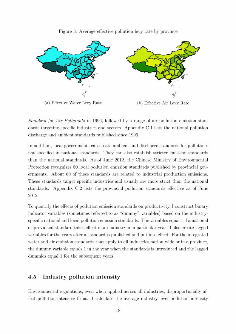
Figure 3: Average effective pollution levy rate by province

(a) Effective Water Levy Rate (b) Effective Air Levy Rate

Standard for Air Pollutants in 1996, followed by a range of air pollution emission stan-

dards targeting specific industries and sectors. Appendix C.1 lists the national pollution

discharge and ambient standards published since 1996.

In addition, local governments can create ambient and discharge standards for pollutants

not specified in national standards. They can also establish stricter emission standards

than the national standards. As of June 2012, the Chinese Ministry of Environmental

Protection recognizes 80 local pollution emission standards published by provincial gov-

ernments. About 60 of these standards are related to industrial production emissions.

These standards target specific industries and usually are more strict than the national

standards. Appendix C.2 lists the provincial pollution standards effective as of June

2012.

To quantify the effects of pollution emission standards on productivity, I construct binary

indicator variables (sometimes referred to as “dummy” variables) based on the industry-

specific national and local pollution emission standards. The variables equal 1 if a national

or provincial standard takes effect in an industry in a particular year. I also create lagged

variables for the years after a standard is published and put into effect. For the integrated

water and air emission standards that apply to all industries nation-wide or in a province,

the dummy variable equals 1 in the year when the standards is introduced and the lagged

dummies equal 1 for the subsequent years.

4.5 Industry pollution intensity

Environmental regulations, even when applied across all industries, disproportionally af-

fect pollution-intensive firms. I calculate the average industry-level pollution intensity

18

in order to capture the degrees to which industries are affected by the environmental

regulations.

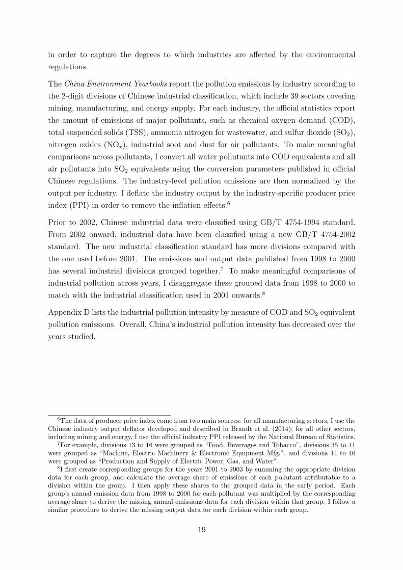
The China Environment Yearbooks report the pollution emissions by industry according to

the 2-digit divisions of Chinese industrial classification, which include 39 sectors covering

mining, manufacturing, and energy supply. For each industry, the official statistics report

the amount of emissions of major pollutants, such as chemical oxygen demand (COD),

total suspended solids (TSS), ammonia nitrogen for wastewater, and sulfur dioxide (SO2),

nitrogen oxides (NOx), industrial soot and dust for air pollutants. To make meaningful

comparisons across pollutants, I convert all water pollutants into COD equivalents and all

air pollutants into SO2 equivalents using the conversion parameters published in official

Chinese regulations. The industry-level pollution emissions are then normalized by the

output per industry. I deflate the industry output by the industry-specific producer price

index (PPI) in order to remove the inflation effects.6

Prior to 2002, Chinese industrial data were classified using GB/T 4754-1994 standard.

From 2002 onward, industrial data have been classified using a new GB/T 4754-2002

standard. The new industrial classification standard has more divisions compared with

the one used before 2001. The emissions and output data published from 1998 to 2000

has several industrial divisions grouped together.7 To make meaningful comparisons of

industrial pollution across years, I disaggregate these grouped data from 1998 to 2000 to

match with the industrial classification used in 2001 onwards.8

Appendix D lists the industrial pollution intensity by measure of COD and SO2 equivalent

pollution emissions. Overall, China’s industrial pollution intensity has decreased over the

years studied.

6The data of producer price index come from two main sources: for all manufacturing sectors, I use theChinese industry output deflator developed and described in Brandt et al. (2014); for all other sectors,including mining and energy, I use the official industry PPI released by the National Bureau of Statistics.

7For example, divisions 13 to 16 were grouped as “Food, Beverages and Tobacco”, divisions 35 to 41were grouped as “Machine, Electric Machinery & Electronic Equipment Mfg.”, and divisions 44 to 46were grouped as “Production and Supply of Electric Power, Gas, and Water”.

8I first create corresponding groups for the years 2001 to 2003 by summing the appropriate divisiondata for each group, and calculate the average share of emissions of each pollutant attributable to adivision within the group. I then apply these shares to the grouped data in the early period. Eachgroup’s annual emission data from 1998 to 2000 for each pollutant was multiplied by the correspondingaverage share to derive the missing annual emissions data for each division within that group. I follow asimilar procedure to derive the missing output data for each division within each group.

19

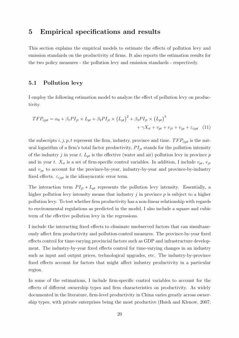
5 Empirical specifications and results

This section explains the empirical models to estimate the effects of pollution levy and

emission standards on the productivity of firms. It also reports the estimation results for

the two policy measures - the pollution levy and emission standards - respectively.

5.1 Pollution levy

I employ the following estimation model to analyze the effect of pollution levy on produc-

tivity.

TFPijpt = α0 + β1PIjt × Lpt + β2PIjt ×(Lpt)2

+ β3PIjt ×(Lpt)3

+ γXit + vpt + vjt + vjp + εijpt (11)

the subscripts i, j, p, t represent the firm, industry, province and time. TFPijpt is the nat-

ural logarithm of a firm’s total factor productivity, PIjt stands for the pollution intensity

of the industry j in year t, Lpt is the effective (water and air) pollution levy in province p

and in year t. Xit is a set of firm-specific control variables. In addition, I include vpt, vjt

and vjp to account for the province-by-year, industry-by-year and province-by-industry

fixed effects. εijpt is the idiosyncratic error term.

The interaction term PIjt ∗ Lpt represents the pollution levy intensity. Essentially, a

higher pollution levy intensity means that industry j in province p is subject to a higher

pollution levy. To test whether firm productivity has a non-linear relationship with regards

to environmental regulations as predicted in the model, I also include a square and cubic

term of the effective pollution levy in the regressions.

I include the interacting fixed effects to eliminate unobserved factors that can simultane-

ously affect firm productivity and pollution-control measures. The province-by-year fixed

effects control for time-varying provincial factors such as GDP and infrastructure develop-

ment. The industry-by-year fixed effects control for time-varying changes in an industry

such as input and output prices, technological upgrades, etc. The industry-by-province

fixed effects account for factors that might affect industry productivity in a particular

region.

In some of the estimations, I include firm-specific control variables to account for the

effects of different ownership types and firm characteristics on productivity. As widely

documented in the literature, firm-level productivity in China varies greatly across owner-

ship types, with private enterprises being the most productive (Hsieh and Klenow, 2007;

20

Song et al., 2011). Moreover, the size of a firm, the number of years since its establish-

ment, whether the firm exports to foreign markets and the capital-labor ratio could also

affect productivity (Syverson, 2011). I include the ownership type, firm size, age, export

status and capital-labor ratio to control for the factors likely to affect the productivity of

a firm.

The size of a firm is defined by the number of employees. The capital labor ratio is defined

as the capital stock divided by the number of employees. The age is the number of years

since the firm was established. A binary indicator variable Foreign equals 1 if more than

25% of the firm’s registered capital is from investors outside of China; hkmctw indicates

if an enterprise has over 25% of its capital from investors based in Hong Kong, Macao

or Taiwan; S.O.E. indicates a state-owned enterprise if over 51% of the registered capital

is state-owned; variable Private equals 1 if over 50% of the firm’s registered capital is

privately owned; Exporter equals 1 if the firm export to a foreign market.

Table 4 reports the estimates for the water and air pollution levy rates. Columns (1)

to (3) report the regression results without firm control variables, and columns (4) to

(6) report the results with firm-specific control variables. I include the equivalent water

and air pollution intensities interacting with the linear, quadratic and cubic forms of the

effective pollution levy.

Looking at the water pollution levy first, when excluding firm control variables, the simple

interaction of the water pollution levy and industrial pollution intensity is not statistically

significant. However, in column (2) the quadratic term of the effective water pollution

levy interacting with pollution intensity displays a statistically significant relationship

with productivity at a 95% confidence interval. In column (3), where I also include the

cubic term of the effective water pollution levy, the coefficients of the linear, quadratic

and cubic terms are all statistically significant. The results display a similar pattern when

control variables are included.

A positive coefficient of the quadratic term and negative coefficients of the linear and cubic

terms indicate a bell-shaped relationship between the pollution levy and firm productivity.

As the levy rate increases, TFP first increases and then goes down beyond a certain point.

Based on the estimation results, Appendix A plots the relationship between the pollution

levy and TFP. A turning point appears at 3.5 RMB. For a pollution levy rate below that

point, an increase in pollution levy is associated with a increase in total factor productivity.

When the water pollution levy rate is above 3.5 RMB, total factor productivity decreases

with the pollution levy. The unit can be roughly interpreted as pollution levy per thousand

RMB output, since the explanatory variable is measured by effective pollution levy (RMB

per kg pollution emission) times industry pollution intensity (kg pollution per thousand

21

Table 4: Water and Air Levy Rate on TFP

(1) (2) (3) (4) (5) (6)TFP TFP TFP TFP TFP TFP

COD Equivalent Pollution Intensity

× Water Levy 0.0013 -0.0014 -0.0064∗∗ 0.0018 -0.0002 -0.0045∗

(0.0012) (0.0017) (0.0027) (0.0012) (0.0017) (0.0026)

× Water Levy2 0.0020∗∗ 0.0085∗∗∗ 0.0015 0.0070∗∗

(0.0009) (0.0029) (0.0009) (0.0029)

× Water Levy3 -0.0014∗∗ -0.0012∗∗

(0.0006) (0.0006)

SO2 Equivalent Pollution Intensity

× Air Levy -0.0062∗∗∗ -0.0141∗∗∗ -0.0208∗∗∗ -0.0069∗∗∗ -0.0135∗∗∗ -0.0181∗∗∗

(0.0012) (0.0026) (0.0037) (0.0012) (0.0025) (0.0037)

× Air Levy2 0.0066∗∗∗ 0.0206∗∗∗ 0.0055∗∗∗ 0.0151∗∗

(0.0019) (0.0063) (0.0019) (0.0062)

× Air Levy3 -0.0075∗∗ -0.0051(0.0033) (0.0033)

S.O.E. -0.1653∗∗∗ -0.1653∗∗∗ -0.1653∗∗∗

(0.0023) (0.0023) (0.0023)

Foreign 0.0002 0.0002 0.0002(0.0023) (0.0023) (0.0023)

Hong Kong, Macao, Taiwan -0.0619∗∗∗ -0.0619∗∗∗ -0.0619∗∗∗

-invested (0.0022) (0.0022) (0.0022)

Private 0.0204∗∗∗ 0.0204∗∗∗ 0.0204∗∗∗

(0.0012) (0.0012) (0.0012)

Size 0.0629∗∗∗ 0.0629∗∗∗ 0.0629∗∗∗

(0.0027) (0.0027) (0.0027)

Exporter -0.0739∗∗∗ -0.0739∗∗∗ -0.0739∗∗∗

(0.0014) (0.0014) (0.0014)

Capital-labor ratio -0.0000∗∗ -0.0000∗∗ -0.0000∗∗

(0.0000) (0.0000) (0.0000)

Age -0.0060∗∗∗ -0.0060∗∗∗ -0.0060∗∗∗

(0.0001) (0.0001) (0.0001)

Province#Year FE Yes Yes Yes Yes Yes YesIndustry#Year FE Yes Yes Yes Yes Yes YesIndustry#Province FE Yes Yes Yes Yes Yes YesObservations 2092038 2092038 2092038 2091663 2091663 2091663R2 0.1071 0.1071 0.1071 0.1236 0.1236 0.1236F 14.7618 11.7539 9.6628 3140.8290 2618.2590 2244.6553

Standard errors in parentheses∗ p < 0.10, ∗∗ p < 0.05, ∗∗∗ p < 0.01

22

RMB output).

The effect of the air pollution levy on total factor productivity suggest a more clear

negative correlation. The linear term of the levy interacting with air pollution intensity

is negatively correlated with productivity, suggesting that a negative relationship exists

between the air pollution levy and firm productivity. On average, a one-unit increase in

the effective pollution levy is associated with a drop of 0.6% in total factor productivity.

The interaction of industry pollution intensity with the quadratic and cubic terms of the

air pollution levy is also significantly correlated with firm productivity. I plot the cubic

and quadratic relationship of the air pollution levy and productivity in Appendix A.

In general, I find a bell-shaped relationship between water pollution levy and productivity,

while air pollution levy displays a more clear negative correlation with productivity. At

first glance, it may seem paradoxical that higher productivity can be associated with a

higher pollution levy. However, the theoretical model discussed in Section 3 presents such

a possibility: when the pollution levy is low, firms may opt for paying the pollution levy

or for diverting some of their resources towards pollution abatement, resulting in lower

productivity. However, when the pollution levy rate is above a certain level, firms may

find it more profitable to switch to new, cleaner technologies, resulting in both reductions

in pollution and increases in productivity.

5.2 Pollution emission standards

In this part of the analysis, I estimate the effects of regulatory pollution emission standards

on firm productivity using the following linear model:

TFPijpt = αjt +T∑t=1

βtSjpt + µi + εijpt (12)

where the subscripts i, j, p, t indicate firm, industry, province and time. TFPijpt is the

natural logarithm of a firm’s total factor productivity. Sjpt is a set of binary indicator

variables that equal 1 if an industry-specific pollution standard is put into effect in industry

j by province p during a specific year t. Sjpt equals one for all provinces if a nation-wide

industry pollution emission standard is introduced in industry j during year t. The

indicator variable equals zero otherwise. Lagged binary variables are also included for

the years after the standards were introduced to capture the dynamic effect of pollution

emission standards.

To control for omitted unobserved variables at the firm and sectoral level, I estimate the

equation in first difference to eliminate time-invariant plant and sector heterogeneity. In

23

order to control for time-varying industry trends that might affect productivity and pollu-

tion emission standards, I include in the differenced question two-digit industry dummies

that account for unobserved trends at broad sector levels.

∆TFPijp = ∆αj +T∑t=1

βt∆Sjp + ∆εijp (13)

Still, there can still be important differences between provinces that are likely to affect

environmental standards. In order to control for these factors, I include in some specifica-

tions the following control variables: per capita GDP of the province, the effective water

and air pollution levies as indicators of environmental stringencies in the province.

∆TFPijp = ∆αj +T∑t=1

βt∆Sjp + γ1GDPpt + γ2Lpt + ∆εijp (14)

Table 5 reports the effects of industry-specific pollution emission standards. Standard year

1 equal 1 when an industry pollution standard took effect in a region and Standard year

2 to 6 indicate the subsequent years after the issuance of an industry pollution standard.

Column (1) reports the lagged effects of an industry pollution standard for four years

and column (2) reports the lagged effects six years following the adoption of a standard.

Columns (3) and column (4) present the results of the same specifications including the

per capita GDP of the province as control. Columns (5) and column (6) report results

including both per capita GDP and effective water/air pollution levy by province.

A negative and significant coefficient of around -0.02 to -0.04 can be observed in the

first year when a regulatory standard is introduced. The coefficient suggests that the

issuance of an industry-specific pollution standard is associated with a decline in the total

factor productivity of 2-4 percentage points for the affected industry in the year when the

standard is put into effect. The negative effect gradually declines over the years and turns

insignificant the third year following the introduction of the environmental standard.

The findings confirm the prediction that a pollution emission standard can lead to an

initial decline in productivity but that it eventually induce firms to improve productivity

in the long run.

24

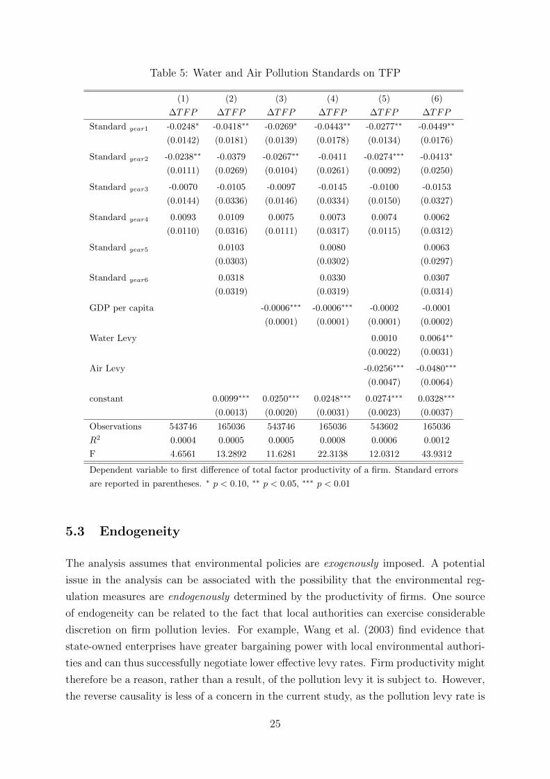
Table 5: Water and Air Pollution Standards on TFP

(1) (2) (3) (4) (5) (6)

∆TFP ∆TFP ∆TFP ∆TFP ∆TFP ∆TFP

Standard year1 -0.0248∗ -0.0418∗∗ -0.0269∗ -0.0443∗∗ -0.0277∗∗ -0.0449∗∗

(0.0142) (0.0181) (0.0139) (0.0178) (0.0134) (0.0176)

Standard year2 -0.0238∗∗ -0.0379 -0.0267∗∗ -0.0411 -0.0274∗∗∗ -0.0413∗

(0.0111) (0.0269) (0.0104) (0.0261) (0.0092) (0.0250)

Standard year3 -0.0070 -0.0105 -0.0097 -0.0145 -0.0100 -0.0153

(0.0144) (0.0336) (0.0146) (0.0334) (0.0150) (0.0327)

Standard year4 0.0093 0.0109 0.0075 0.0073 0.0074 0.0062

(0.0110) (0.0316) (0.0111) (0.0317) (0.0115) (0.0312)

Standard year5 0.0103 0.0080 0.0063

(0.0303) (0.0302) (0.0297)

Standard year6 0.0318 0.0330 0.0307

(0.0319) (0.0319) (0.0314)

GDP per capita -0.0006∗∗∗ -0.0006∗∗∗ -0.0002 -0.0001

(0.0001) (0.0001) (0.0001) (0.0002)

Water Levy 0.0010 0.0064∗∗

(0.0022) (0.0031)

Air Levy -0.0256∗∗∗ -0.0480∗∗∗

(0.0047) (0.0064)

constant 0.0099∗∗∗ 0.0250∗∗∗ 0.0248∗∗∗ 0.0274∗∗∗ 0.0328∗∗∗

(0.0013) (0.0020) (0.0031) (0.0023) (0.0037)

Observations 543746 165036 543746 165036 543602 165036

R2 0.0004 0.0005 0.0005 0.0008 0.0006 0.0012

F 4.6561 13.2892 11.6281 22.3138 12.0312 43.9312

Dependent variable to first difference of total factor productivity of a firm. Standard errors

are reported in parentheses. ∗ p < 0.10, ∗∗ p < 0.05, ∗∗∗ p < 0.01

5.3 Endogeneity

The analysis assumes that environmental policies are exogenously imposed. A potential

issue in the analysis can be associated with the possibility that the environmental reg-

ulation measures are endogenously determined by the productivity of firms. One source

of endogeneity can be related to the fact that local authorities can exercise considerable

discretion on firm pollution levies. For example, Wang et al. (2003) find evidence that

state-owned enterprises have greater bargaining power with local environmental authori-

ties and can thus successfully negotiate lower effective levy rates. Firm productivity might

therefore be a reason, rather than a result, of the pollution levy it is subject to. However,

the reverse causality is less of a concern in the current study, as the pollution levy rate is

25

calculated at the provincial-level while total factor productivity is calculated at the firm-

level. It would be difficult to argue that the overall productivity of all polluting firms in

a province would affect the province-wide effective pollution levy.

Another possible source of endogeneity can come from unobserved variables that affect

both firm productivity and the pollution levy. For example, one might expect that in high-

income provinces, firms tend to be more productive and that pollution levies charged tend

to be higher. Out of such concern, I include in the empirical models various fixed effects to

account for factors associated with time-variant effects of location and industry. The rich

fixed effects included in the estimation should largely eliminate any unobserved factors

that affect environmental policy and productivity simultaneously.

6 Conclusions

This paper investigates the effects of two important environmental policy instruments

- the pollution levy and regulatory standards - on firm productivity in China. It finds

evidence in support of the Porter hypothesis that an increase in environmental standards

can actually improve competitiveness under certain circumstances.

The analysis is informed by a theoretical model where a technological upgrade simulta-

neously alleviates pollution and benefits productivity. Without government intervention,

however, firms may be reluctant to upgrade to the new technology due to the switching

costs. The model predicts that tighter environmental regulations can induce firms to

upgrade technology, leading to productivity increase in the long-run. The model shows

Porter’s argument that environmental regulations can simultaneously reduce pollution

and benefit productivity is consistent with economic theory.

To empirically test the hypothesis, I calculate total factor productivity of Chinese indus-

trial firms based on data from the annual survey of industrial enterprises covering 90% of

China’s total manufacturing sales over ten years. I also construct policy indicators for the

provincial-level effective pollution levy, industry pollution intensity and pollution emission

standards based on the statistics published in the China Environment Yearbooks. The

calculated effective pollution levy rates range from 0.01 RMB to 6.7 RMB per kilogram of

water pollution discharges, and from 0.015 RMB to 1.5 RMB per kilogram of air pollution

emissions; significant variations can be observed across provinces and over time.

The empirical analysis of the relationship between the effective pollution levy and firm

productivity finds a positive or non-linear correlation for the water levy. In some of the

estimations, productivity increases with the pollution levy when the levy rate is below

26

3.5 RMB for roughly per thousand RMB output, and decreases when the pollution levy

rate exceeds 3.5 RMB. For the air pollution levy, one can observe a negative correlation

between the levy rate and productivity. On average, a one-unit increase in the pollution

levy is associated with a drop of 0.6% in total factor productivity.

An analysis of China’s regulatory standards finds that emission standards have a negative

initial effect on firm productivity but a positive effect in the long-run. An industry-specific

pollution standard can be associated with a 2-4% reduction in productivity in the same

year that the standard is adopted. The negative effects can last up to three years, but

higher environmental standards eventually diminishes and are sometimes correlated with

higher productivity. The finding is consistent with the Porter hypothesis whereby environ-

mental standards can induce firms to upgrade technology and increase productivity.

The empirical study in this paper focuses on the correlation, not causality, between pol-

lution control policies and productivity. However, as provincial-level pollution levies and

industry-specific pollution emission standards are not likely to be affected by the produc-

tivity of individual firms, the policy measures discussed in the study can be thought of as

largely exogenous.

The empirical analysis in this paper finds evidence in support of the Porter hypothesis.

While similar studies conducted in industrialized countries often find negative correla-

tion between environmental regulations and productivity, the discovery of a positive or

sometimes non-linear relationship between pollution control measures and productivity

in China suggests that environmental regulations can be associated with productivity

increases. As firms in a developing country like China tend to rely on low production

technologies, they are more likely to switch to cleaner and more efficient technologies in

response to stringent environmental regulations.

27

Appendix A - Correlation of pollution levy and TFP

Estimated relationship of water levy and productivity excluding control variables. The blue dots are theactual effective pollution levy rates.

Estimated relationship of water levy and productivity including control variables. The blue dots are theactual effective pollution levy rates.

28

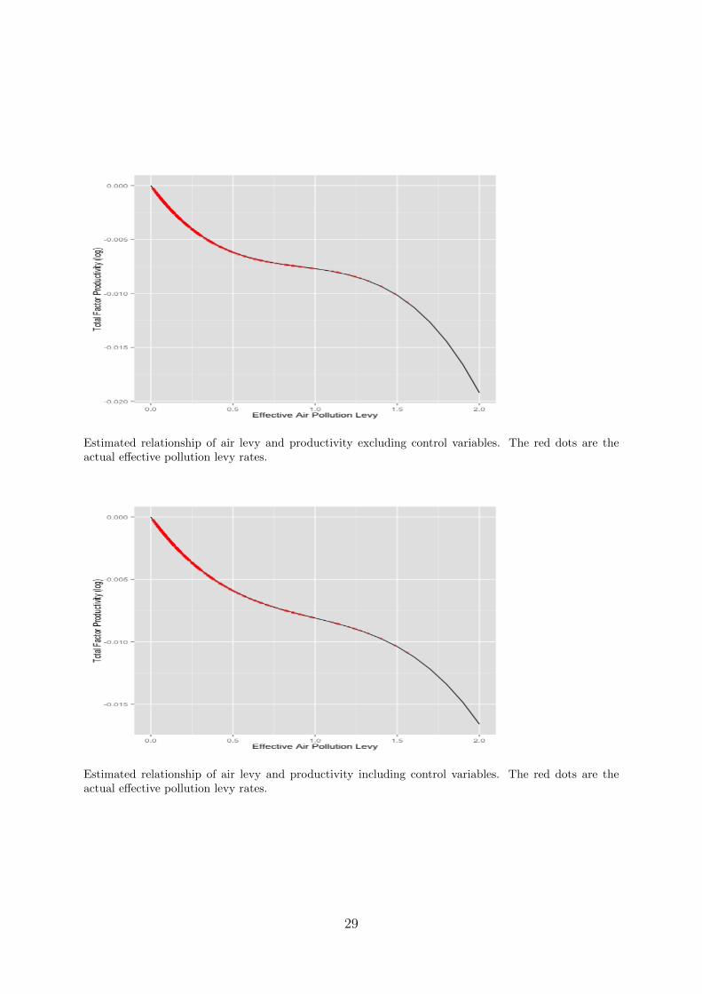
Estimated relationship of air levy and productivity excluding control variables. The red dots are theactual effective pollution levy rates.

Estimated relationship of air levy and productivity including control variables. The red dots are theactual effective pollution levy rates.

29

Appendix B - The pollution levy system in China

This Appendix summarizes China’s pollution levy system, and in particular, a regulatory

change introduced in 2003. Most of the contents are summarized from Wang and Wheeler

(2005) and Jin and Lin (2014).

Discussion of a possible pollution charge system began in China after the 1972 Stockholm

Conference on the Human Environment. In February 1982, the Central Government

of China issued an Interim Procedure on Pollution Charges that defined the system’s

objectives, principles, levy standards, levy collection methods, and the principles for how

funds collected through the levy should be used. Nationwide, the implementation of the

national levy procedure followed rapidly. In January 2003, the State Council of China

passed a new pollution levy regulation which replaced the Interim Procedure. The new

regulation substantially reformed the pollution levy system.

The pollution levy system is based on universal self-reporting, with verification conducted

by local regulatory authorities. At the beginning of the year, plants must register with

environmental authorities by providing basic economic information and their expected

volume of emissions for the coming year. Environmental authorities verify the registration

reports and then issue pollution discharge licenses to plants. During the year, plants are

required to modify their reports if their actual emissions are different from those predicted

at the beginning of the year. Environmental authorities verify plant reports by conducting

field inspections, in most cases without prior warning. At the end of each quarter, based

on plant reports and inspections, authorities announce the pollution levies that plants

should pay at the end of the quarter. False reporting caught by the authorities is subject

to penalties.

Pollution charges are levied for 29 water pollutants and 22 air pollutants, as well as for

solid waste and radioactive waste and noise. Among the pollutants, the major focus of

monitoring and levy collection is on COD (chemical oxygen demand) and TSS (total

suspended solids) for water, and SO2 and flue dust for the air.

Pre-2003 pollution levy system

The evolution of China’s pollution levy system can be divided into two distinct periods:

pre- and post-2003. Table 6 summarizes the composition of the levy collections in China

from 1992 to 2002.

Prior to 2003, water pollution charges contributed the largest share of the total pollution

levies. The water pollution levy charge varies by both the concentration of hazardous

30

chemicals and the volume of wastewater.

Table 6: Pollution levy collection in China, 1992-2002(10 000 RMB)

Year Total From Emissions above standards From From From

Water Air Solid waste Noise Radioactive wastewater penalties SO2 fee

wastes discharge fee

1992 239,452 118,673 50,859 3,079 8,930 1,037 8,485 48,389

1993 268,013 122,838 56,021 3,747 11,930 20 12,637 60,821

1994 309,757 132,197 64,498 3,199 15,551 89 20,046 74,177

1995 371,281 150,365 74,297 4,846 19,019 166 25,384 97,204

1996 409,594 155,135 67,212 3,743 21,413 183 28,791 118,542 14,575

1997 454,332 164,194 67,682 5,015 24,417 151 30,521 139,799 22,553

1998 490,194 163,746 65,491 4,394 26,410 77 28,281 150,285 51,510

1999 554,512 166,521 69,757 5,956 30,549 383 29,089 166,124 86,133

2000 579,607 172,217 76,104 6,998 34,234 472 27,320 184,658 77,603

2001 621,802 175,803 72,052 8,592 34,864 139 23,521 196,475 110,358

2002 674,376 179,524 79,063 8,983 37,539 252 27,920 218,673 122,424

For a plant i that discharges within the pre-specified concentration standards, the levy

for wastewater discharge is based on the total volume of wastewater discharge W and the

levy rate R0. For within-standard polluters, the uniform levy rate is set at 0.05 RMB per

ton of wastewater discharge:

Li = R0Wi (15)

whereas for a plant that exceeds the concentrate standards, the levy formula for wastew-

ater discharges is:

Pij = WiCij − CsjCsj

Lij =

L0j +R1jPij if Pij > Tj

R2jPij if Pij < Tj(16)

where for plant i and pollutant j,

Pij = Discharge factor Wi = Total wastewater discharge

Cij = Pollution concentration Csj = Concentration standard

Lij = Total levy L0j = Fixed payment factor

Tj = Regulatory threshold parameter

R1 and R2 are pollution levy charge standards with R2 > R1; and for continuity at

Tj, R2jTj = L0j + R1jTj. The pollutant concentration standard Cs is jointly set by the

31

central and local governments. The charge rate R is determined relative to a critical

factor T ; both R and T are set by the central government and vary by pollutant, but not

by industry. The potential levy Lj is calculated for each pollutant; the actual levy is the

greatest of the potential levies.

Table 7 lists the national standards on the pollution levy rates R, threshold parameters

T and fixed payment L0j for the most common water pollutants9.

Table 7: Pollution charge standards for common water pollutants

Regulatory Levy Charge Levy Charge Fixed Payment

Pollutant Threshold Tj Standard R2 Standard R1 Factor L0j

(RMB/tons) (RMB/tons) (RMB)

COD 20000 0.18 0.05 2600

TSS 800000 0.03 0.01 16000

Mercury 2000 2.00 1.00 2000

Cadmium 3000 1.00 0.15 2550

Petroleum 25000 0.20 0.06 3500

Ammonia Nitrogen 25000 0.10 0.03 1750

Hexavalent Chrome 150000 0.09 0.02 10500

Arsenic 150000 0.09 0.02 10500

Lead 150000 0.08 0.03 7500

Volatile Hydroxybenzene 250000 0.06 0.03 7500

Cyanide 250000 0.07 0.04 7500

Sulfide 250000 0.05 0.02 7500

The levy formula for air pollution is

Lij = Max[0, RjVi(Cij − Csj)

](17)

where, for plant i and pollutant j, Rj is the charge rate for pollutant j, Vi the total volume

of air emissions, Cij the pollution concentration, Csj the concentration standard, Lij the

total levy. The charge is zero when the pollutant concentration C is less than or equal to

the standard Cs. Unlike the water levy, the air levy is assessed on the absolute, rather

than percentage, deviation from the concentration standard. Again, a firm is assessed

only by the highest of its potential levies.

There are four major sources of provincial variation in pollution tax rates. First, as noted

above, concentration standards Csj are set jointly by the national and local governments

and can vary by region. Second, the standard differs by pollutant, thus differences in

the concentration of industries across provinces will lead to different effective levy rates.

9NEPA, SPB, and MOF (National Environmental Protection Agency, State Price Bureau and Ministryof Finance), 1991, A Notice on Adjustment of the Pollution Discharge Fee Rate for Wastewater and thePollution Levy Rate for Noise. Document 262-91, Beijing.

32

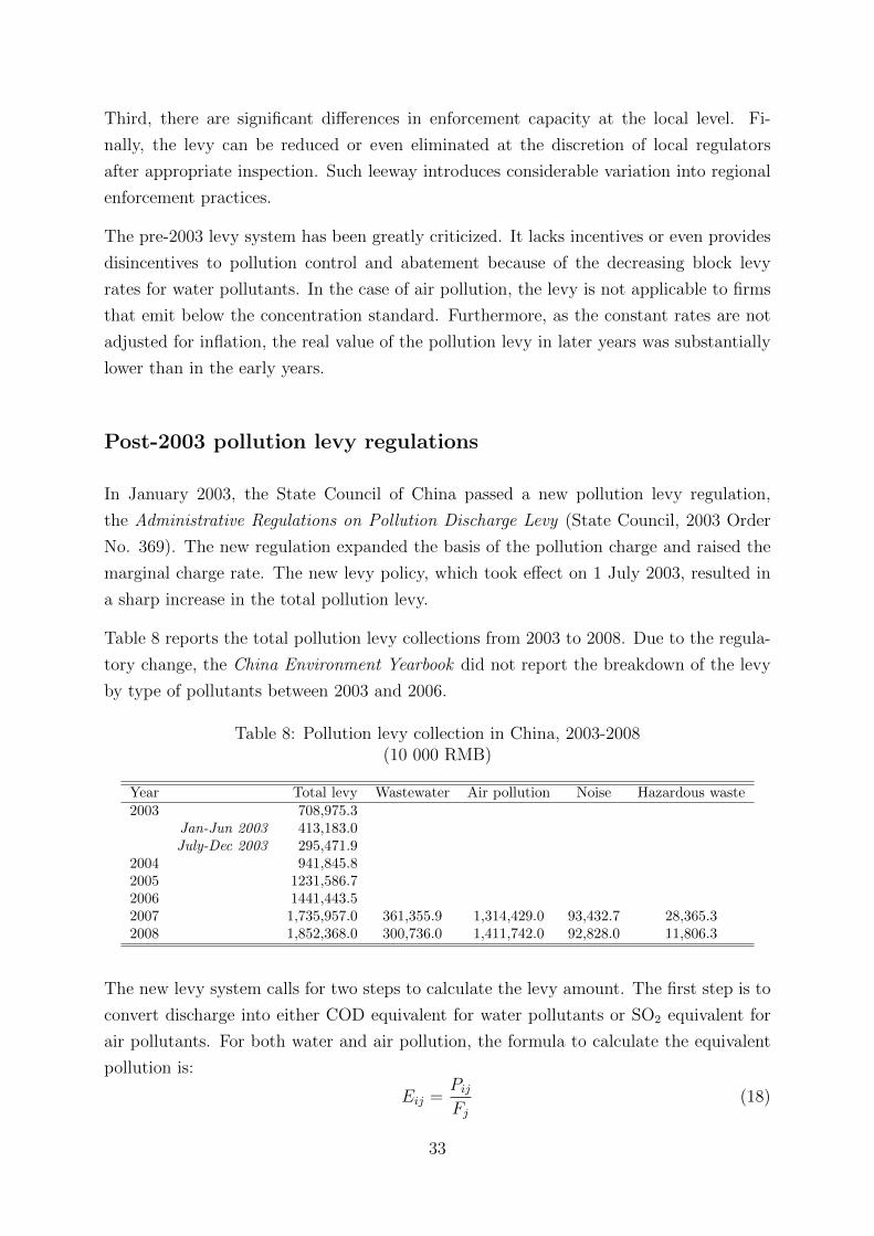
Third, there are significant differences in enforcement capacity at the local level. Fi-

nally, the levy can be reduced or even eliminated at the discretion of local regulators

after appropriate inspection. Such leeway introduces considerable variation into regional

enforcement practices.

The pre-2003 levy system has been greatly criticized. It lacks incentives or even provides

disincentives to pollution control and abatement because of the decreasing block levy

rates for water pollutants. In the case of air pollution, the levy is not applicable to firms

that emit below the concentration standard. Furthermore, as the constant rates are not

adjusted for inflation, the real value of the pollution levy in later years was substantially

lower than in the early years.

Post-2003 pollution levy regulations

In January 2003, the State Council of China passed a new pollution levy regulation,

the Administrative Regulations on Pollution Discharge Levy (State Council, 2003 Order

No. 369). The new regulation expanded the basis of the pollution charge and raised the

marginal charge rate. The new levy policy, which took effect on 1 July 2003, resulted in

a sharp increase in the total pollution levy.

Table 8 reports the total pollution levy collections from 2003 to 2008. Due to the regula-

tory change, the China Environment Yearbook did not report the breakdown of the levy

by type of pollutants between 2003 and 2006.

Table 8: Pollution levy collection in China, 2003-2008(10 000 RMB)

Year Total levy Wastewater Air pollution Noise Hazardous waste2003 708,975.3

Jan-Jun 2003 413,183.0July-Dec 2003 295,471.9

2004 941,845.82005 1231,586.72006 1441,443.52007 1,735,957.0 361,355.9 1,314,429.0 93,432.7 28,365.32008 1,852,368.0 300,736.0 1,411,742.0 92,828.0 11,806.3

The new levy system calls for two steps to calculate the levy amount. The first step is to

convert discharge into either COD equivalent for water pollutants or SO2 equivalent for

air pollutants. For both water and air pollution, the formula to calculate the equivalent

pollution is:

Eij =PijFj

(18)

33

where Eij is the equivalent discharge for pollutant j; Pij is the emission/discharge of

pollutant j in plant i, and Fj is a conversion parameter for pollutant j. The equivalent

discharge for each pollutant j is calculated as the plant i’s total emission of pollutant

j (in kg) divided by the conversion parameter Fj. The pollutants that are more likely

to cause environmental damage are assigned a smaller conversion parameter and have

greater amount of the equivalents.

The new formula suggests that any polluter needs to pay for pollution discharge, regardless

if their emission meets the concentration standard. Table 9 lists the conversion parameter

Fj for selected water and air pollutants.

Table 9: Pollution conversion parameter for selected pollutants

Pollutant conversion parameter Fj (kg)

Water pollutants:

COD 1

TSS 4

Petroleum 0.1

Ammonia Nitrogen 0.8

Mercury 0.0005

Cadmium 0.005

Hexavalent Chrome 0.02

Arsenic 0.02

Lead 0.025

Volatile Hydroxybenzene 0.08

Cyanide 0.05

Sulfide 0.125

Air pollutants:

SO2 0.95

NOx 0.95

CO 16.7

Chlorine 0.34

Dust 4

Soot 2.18

Under the new pollution levy regulation, plants are required to pay levies on the sum of

the highest three of the calculated pollution equivalents. The second step to calculate the

pollution levy is:

Li = Rj ∗3∑j=1

Eij (19)

where Rj is the marginal levy rate, and the total pollution levy Li is for plant i will

be the marginal levy rate multiplying the sum of the three highest calculated potential

charges.

For water pollutants, the marginal levy rate Rj equals 0.7 RMB per unit of COD equiva-

34

lent, and for air pollutants, the marginal levy rate is 0.6 RMB per unit of SO2 equivalent

for the within-standard discharge. The rates are doubled for discharges that are higher

than the standards, i.e. 1.4 RMB and 1.2 RMB for COD and SO2 equivalent, respec-

tively.

To illustrate the difference between the pre- and post-2003 levy systems, I assume there

are two plants, each emitting a total of 500,000 tons of wastewater with three particular

pollutants: COD, TSS and Ammonia Nitrogen. One plant emits within the standards

and the other exceeds the standards. Table 10 shows the potential levy charge under

the pre- and post-2003 regulations. For the within-standard polluter, the levy under the

new pollution regulation increased slightly. For the above-standard polluter, the levy

under the new regulation is almost five times the levy under the pre-2003 regulations.

The comparisons show that the post-2003 system penalizes heavy polluters substantially

more.

Table 10: Comparison of potential levy under different pollution levy regulations

Actual Concentration Pollutant Levy Amount

Concentration Standard Discharge Pre-2003 Post-2003

(mg/L) (mg/L) (kg) (RMB) (RMB)

Within-standard polluter:

COD 50 100 25,000 17,500

TSS 50 70 25,000 4,375

Ammonia Nitrogen 10 30 5,000 4,375

Total actual levy (RMB) 25,000 26,250

Above-standard polluter:

COD 200 100 100,000 27,600 103,500

TSS 350 70 175,000 36,000 55,125

Ammonia Nitrogen 50 30 25,000 2,500 21,875

Total actual levy (RMB) 36,000 180,600

35

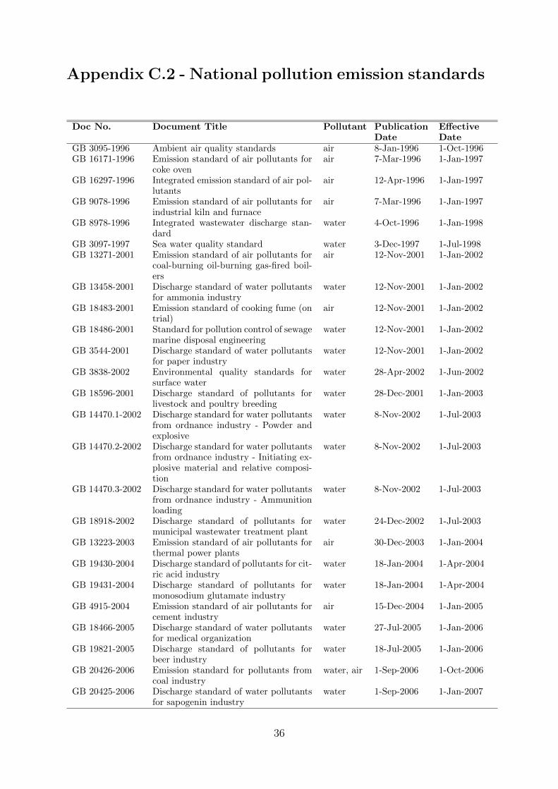
Appendix C.2 - National pollution emission standards

Doc No. Document Title Pollutant PublicationDate

EffectiveDate

GB 3095-1996 Ambient air quality standards air 8-Jan-1996 1-Oct-1996GB 16171-1996 Emission standard of air pollutants for

coke ovenair 7-Mar-1996 1-Jan-1997

GB 16297-1996 Integrated emission standard of air pol-lutants

air 12-Apr-1996 1-Jan-1997

GB 9078-1996 Emission standard of air pollutants forindustrial kiln and furnace

air 7-Mar-1996 1-Jan-1997

GB 8978-1996 Integrated wastewater discharge stan-dard

water 4-Oct-1996 1-Jan-1998

GB 3097-1997 Sea water quality standard water 3-Dec-1997 1-Jul-1998GB 13271-2001 Emission standard of air pollutants for

coal-burning oil-burning gas-fired boil-ers

air 12-Nov-2001 1-Jan-2002

GB 13458-2001 Discharge standard of water pollutantsfor ammonia industry

water 12-Nov-2001 1-Jan-2002

GB 18483-2001 Emission standard of cooking fume (ontrial)

air 12-Nov-2001 1-Jan-2002

GB 18486-2001 Standard for pollution control of sewagemarine disposal engineering

water 12-Nov-2001 1-Jan-2002

GB 3544-2001 Discharge standard of water pollutantsfor paper industry

water 12-Nov-2001 1-Jan-2002

GB 3838-2002 Environmental quality standards forsurface water

water 28-Apr-2002 1-Jun-2002

GB 18596-2001 Discharge standard of pollutants forlivestock and poultry breeding

water 28-Dec-2001 1-Jan-2003

GB 14470.1-2002 Discharge standard for water pollutantsfrom ordnance industry - Powder andexplosive

water 8-Nov-2002 1-Jul-2003

GB 14470.2-2002 Discharge standard for water pollutantsfrom ordnance industry - Initiating ex-plosive material and relative composi-tion

water 8-Nov-2002 1-Jul-2003

GB 14470.3-2002 Discharge standard for water pollutantsfrom ordnance industry - Ammunitionloading

water 8-Nov-2002 1-Jul-2003

GB 18918-2002 Discharge standard of pollutants formunicipal wastewater treatment plant

water 24-Dec-2002 1-Jul-2003

GB 13223-2003 Emission standard of air pollutants forthermal power plants

air 30-Dec-2003 1-Jan-2004

GB 19430-2004 Discharge standard of pollutants for cit-ric acid industry

water 18-Jan-2004 1-Apr-2004

GB 19431-2004 Discharge standard of pollutants formonosodium glutamate industry

water 18-Jan-2004 1-Apr-2004

GB 4915-2004 Emission standard of air pollutants forcement industry

air 15-Dec-2004 1-Jan-2005

GB 18466-2005 Discharge standard of water pollutantsfor medical organization

water 27-Jul-2005 1-Jan-2006

GB 19821-2005 Discharge standard of pollutants forbeer industry

water 18-Jul-2005 1-Jan-2006

GB 20426-2006 Emission standard for pollutants fromcoal industry

water, air 1-Sep-2006 1-Oct-2006

GB 20425-2006 Discharge standard of water pollutantsfor sapogenin industry

water 1-Sep-2006 1-Jan-2007

36

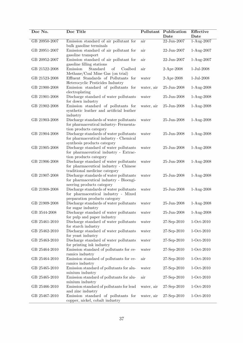
Doc No. Doc Title Pollutant PublicationDate

EffectiveDate

GB 20950-2007 Emission standard of air pollutant forbulk gasoline terminals

air 22-Jun-2007 1-Aug-2007

GB 20951-2007 Emission standard of air pollutant forgasoline transport

air 22-Jun-2007 1-Aug-2007

GB 20952-2007 Emission standard of air pollutant forgasoline filling stations

air 22-Jun-2007 1-Aug-2007

GB 21522-2008 Emission Standard of CoalbedMethane/Coal Mine Gas (on trial)

air 2-Apr-2008 1-Jul-2008

GB 21523-2008 Effluent Standards of Pollutants forHeterocyclic Pesticides Industry

water 2-Apr-2008 1-Jul-2008

GB 21900-2008 Emission standard of pollutants forelectroplating

water, air 25-Jun-2008 1-Aug-2008

GB 21901-2008 Discharge standard of water pollutantsfor down industry

water 25-Jun-2008 1-Aug-2008

GB 21902-2008 Emission standard of pollutants forsynthetic leather and artificial leatherindustry

water, air 25-Jun-2008 1-Aug-2008

GB 21903-2008 Discharge standards of water pollutantsfor pharmaceutical industry- Fermenta-tion products category

water 25-Jun-2008 1-Aug-2008

GB 21904-2008 Discharge standards of water pollutantsfor pharmaceutical industry - Chemicalsynthesis products category

water 25-Jun-2008 1-Aug-2008

GB 21905-2008 Discharge standard of water pollutantsfor pharmaceutical industry - Extrac-tion products category

water 25-Jun-2008 1-Aug-2008

GB 21906-2008 Discharge standard of water pollutantsfor pharmaceutical industry - Chinesetraditional medicine category

water 25-Jun-2008 1-Aug-2008

GB 21907-2008 Discharge standards of water pollutantsfor pharmaceutical industry - Bioengi-neering products category

water 25-Jun-2008 1-Aug-2008

GB 21908-2008 Discharge standards of water pollutantsfor pharmaceutical industry - Mixedpreparation products category

water 25-Jun-2008 1-Aug-2008

GB 21909-2008 Discharge standards of water pollutantsfor sugar industry

water 25-Jun-2008 1-Aug-2008

GB 3544-2008 Discharge standard of water pollutantsfor pulp and paper industry

water 25-Jun-2008 1-Aug-2008

GB 25461-2010 Discharge standard of water pollutantsfor starch industry

water 27-Sep-2010 1-Oct-2010

GB 25462-2010 Discharge standard of water pollutantsfor yeast industry

water 27-Sep-2010 1-Oct-2010

GB 25463-2010 Discharge standard of water pollutantsfor printing ink industry

water 27-Sep-2010 1-Oct-2010

GB 25464-2010 Emission standard of pollutants for ce-ramics industry

water 27-Sep-2010 1-Oct-2010

GB 25464-2010 Emission standard of pollutants for ce-ramics industry

air 27-Sep-2010 1-Oct-2010

GB 25465-2010 Emission standard of pollutants for alu-minium industry

water 27-Sep-2010 1-Oct-2010

GB 25465-2010 Emission standard of pollutants for alu-minium industry

air 27-Sep-2010 1-Oct-2010

GB 25466-2010 Emission standard of pollutants for leadand zinc industry

water, air 27-Sep-2010 1-Oct-2010

GB 25467-2010 Emission standard of pollutants forcopper, nickel, cobalt industry

water, air 27-Sep-2010 1-Oct-2010

37

Doc No. Doc Title Pollutant PublicationDate

EffectiveDate

GB 25468-2010 Emission standard of pollutants formagnesium and titanium industry

water, air 27-Sep-2010 1-Oct-2010

GB 26131-2010 Emission standard of pollutants for ni-tric acid industry

water, air 30-Dec-2010 1-Mar-2011

GB 26132-2010 Emission standard of pollutants for sul-phuric acid industry

water, air 30-Dec-2010 1-Mar-2011

GB 15580-2011 Discharge standard of water pollutantsfor phosphate fertilizer industry

water 2-Apr-2011 1-Oct-2011

GB 26451-2011 Emission Standards of pollutants fromrare earths industry

water, air 24-Jan-2011 1-Oct-2011

GB 26452-2011 Discharge standard of pollutants forvanadium Industry

water, air 2-Apr-2011 1-Oct-2011

GB 26453-2011 Emission standard of air pollutants forflat glass industry

air 11-Apr-2011 1-Oct-2011

GB 13223-2011 Emission standard of air pollutants forthermal power plants

air 29-Jul-2011 1-Jan-2012

GB 14470.3-2011 Effluent standards of water pollutantsfor ammunition loading industry

water 29-Apr-2011 1-Jan-2012

GB 26877-2011 Discharge standard of water pollutantsfor motor vehicle maintenance and re-pair

water 2-Jul-2011 1-Jan-2012

GB 27631-2011 Discharge standard of water pollutantsfor fermentation alcohol and distilledspirits industry

water 27-Oct-2011 1-Jan-2012

GB 27632-2011 Emission standard of pollutants forrubber products industry

water, air 27-Oct-2011 1-Jan-2012

GB 13456-2012 Discharge standard of water pollutantsfor iron and steel industry

water 27-Jun-2012 1-Oct-2012

GB 16171-2012 Emission standard of pollutants for cok-ing chemical industry

water, air 27-Jun-2012 1-Oct-2012

GB 28661-2012 Emission standard of pollutants formining and mineral processing industry

water, air 27-Jun-2012 1-Oct-2012

GB 28662-2012 Emission standard of air pollutants forsintering and pelletizing of iron andsteel industry

air 27-Jun-2012 1-Oct-2012

GB 28663-2012 Emission standard of air pollutants foriron smelt industry

air 27-Jun-2012 1-Oct-2012

GB 28664-2012 Emission standard of air pollutants forsteel smelt industry

air 27-Jun-2012 1-Oct-2012

GB 28666-2012 Emission standard of pollutants for fer-roalloy smelt industry

water, air 27-Jun-2012 1-Oct-2012

GB 28936-2012 Discharge standards of water pollutantsfor reeling industry

water 19-Oct-2012 1-Jan-2013

GB 28937-2012 Discharge standards of water pollutantsfor woolen textile industry

water 19-Oct-2012 1-Jan-2013

GB 28938-2012 Discharge standards of water pollutantsfor bast and leaf fibres textile industry

water 19-Oct-2012 1-Jan-2013

GB 4287-2012 Discharge standards of water pollutantsfor dyeing and finishing of textile indus-try

water 19-Oct-2012 1-Jan-2013

GB 13458-2001 Discharge standard of water pollutantsfor ammonia industry

water 14-Mar-2013 1-Jul-2013

GB 19430-2013 Effluent standards of water pollutantsfor citric acid industry

water 14-Mar-2013 1-Jul-2013

GB 28665-2012 Emission standard of air pollutants forsteel rolling industry

air 14-Mar-2013 1-Jul-2013

GB 29495-2013 Emission standard of air pollutants forelectronic glass industry

air 14-Mar-2013 1-Jul-2013

38

Appendix C.2 - Provincial emission standards

Doc No. Province Document Title Pollutant EffectiveDate

DB11/206-2003 Beijing Emission Controls and Limits for Gaso-line Vapor on Bulk Gasoline Terminals

air 2003.10.01

DB11/207-2003 Beijing Emission Controls and Limits for Gaso-line Vapor on Tank Truck

air 2003.10.01

DB11/208-2003 Beijing Emission Controls and Limits for Gaso-line Vapor on Gasoline Filling Station

air 2003.10.01

DB11/307-2005 Beijing Discharge Standard of Water Pollu-tants

water 2005.09.01

DB11/447-2007 Beijing Emission Standards of Air Pollutantsfor Petroleum Refining and Petrochem-icals Manufacturing Industry

air 2007.07.01

DB11/139-2007 Beijing Emission Standard of Air Pollutants forBoilers

air 2007.09.01

DB11/501-2007 Beijing Integrated Emission Standards of AirPollutants

air 2008.01.01

DB11/502-2007 Beijing Emission Standard of Air Pollutants forMunicipal Solid Wastes Incineration

air 2008.01.01

DB11/503-2007 Beijing Emission Standard of Air Pollutants forHazardous Wastes Incineration

air 2008.01.01

DB11/206-2010 Beijing Emission Controls and Limits for Gaso-line Vapor on Bulk Gasoline Terminals

air 2010.07.01

DB11/207-2010 Beijing Emission Controls and Limits for Gaso-line Vapor on Tank Truck

air 2010.07.01

DB11/208-2010 Beijing Emission Controls and Limits for Gaso-line Vapor on Gasoline Filling Station

air 2010.07.01

DB11/847-2011 Beijing Emission standard of air pollutants forstationary gas turbine

air 2012.01.01

DB62/1922-2010 Gansu Emission standard for air pollutantsfrom boilers for Lanzhou City

air 2010.06.10

DB44/26-2001 Guangdong Discharge Limits of Water Pollutants water 2002.02.01DB44/27-2001 Guangdong Emission Limits of Air Pollutants air 2002.02.01DB44/612-2009 Guangdong Emission standard of air pollutants for

thermal power plantsair 2009.08.01

DB44/613-2009 Guangdong Discharge standard of pollutants forlivestock and poultry breeding

water, air 2009.08.02

DB44/765-2010 Guangdong Emission Standard of Air Pollutants forBoilers

air 2010.11.01

DB44/814-2010 Guangdong Emission standard of volatile organiccompounds for furniture manufacturingoperations

air 2010.11.02

DB44/815-2010 Guangdong Emission standard of volatile organiccompounds for printing industry

air 2010.11.03

DB44/816- 2010 Guangdong Emission standard of volatile organiccompounds for surface coating of auto-mobiles

air 2010.11.04

DB44/817-2010 Guangdong Emission standard of volatile organiccompounds for shoe-making industry

air 2010.11.05

DB44/818-2010 Guangdong Emission standard of air pollutants forcement industry

air 2010.11.06

DB13/339-1997 Hebei Dust Environmental Quality Standards(Trial)

air 1998.05.01

DB13/831-2006 Hebei Chloride emission standards water 2007.01.01DB13/1200-2010 Hebei Emission standard of air granular mat-

ter for iron ore mineral processing fac-tory

air 2010.05.04

DB13/1461-2011 Hebei Steel industrial air pollutants emissionstandards

air 2011.11.30

39

Doc No. Province Document Title Pollutant EffectiveDate

DB23/1341-2009 Heilongjiang Furfural industrial water pollutant dis-charge standards

2009.08.01

DB41/538-2008 Henan Ammonia industry wastewater dis-charge standards

water 2009.01.01

DB41/681-2011 Henan Beer industrial wastewater dischargestandards

water 2011.11.01

DB41/684-2011 Henan Lead smelting industry emission stan-dards

water, air 2013.01.01

DB32/670-2004 Jiangsu Discharge Standard of Water Pollu-tants for Dyeing and Finishing

water 2005.01.01

DB32/939-2006 Jiangsu Discharge Standard of main water pol-lutants for chemical industry

water 2006.07.26

DB32/1072-2007 Jiangsu Discharge Standard of Main WaterPollutants for Municipal WastewaterTreatment Plant & Key Industries ofTaihu Area

water 2008.01.01

DB21/1627-2008 Liaoning Integrated Wastewater Discharge Stan-dard

water 2008.08.01

DB37/336-2003 Shandong Wastewater discharge standards for pa-per industry

water 2003.05.01

DB37/533-2005 Shandong Discharge Standard of Water Pollu-tants for Dyeing and Finishing

water 2005.05.01

DB37/534-2005 Shandong Emission standards for livestock andpoultry industries

2005.05.01

DB37/532-2005 Shandong Cement industry emission standards ofair pollutants

air 2005.07.01

DB37/597-2006 Shandong Cooking fume emission standards 2006.01.04DB37/664-2007 Shandong Thermal power plant air pollutant

emission standardsair 2007.05.01

DB37/676-2007 Shandong Integrated Wastewater Discharge Stan-dard in Shandong Peninsula Basin

water 2007.10.01

DB37/990-2008 Shandong Iron and steel industry emission stan-dards

water, air 2008.02.01

DB37/1919-2011 Shandong Aluminum industry emission standards air 2011.10.01DB37/2376-2013 Shandong Integrated Emission Standards of Air

Pollutantsair 2013.09.01

DB37/595-2006 Shandong Starch processing industrial water pol-lutant discharge standards

water 2006.01.04

DB31/373-2006 Shanghai Discharge Standard of Pollutants forBio-pharmaceutical Industry

water, air 2006.02.01

DB31/374-2006 Shanghai Discharge Standards of Pollutants forSemiconductor Industry

water, air 2007.02.01

DB31/387-2007 Shanghai Emission standard for air pollutantsfrom boilers

air 2007.09.01

DB31/445-2009 Shanghai Discharge Standard for Municipal Sew-erage System

water 2009.09.01

DB31/199-2009 Shanghai Integrated wastewater discharge stan-dard

water 2009.10.01

DB31/373-2010 Shanghai Discharge Standard of Pollutants forBio-pharmaceutical Industry

water, air 2010.07.01

DB31/ 387-2013 Shanghai Emission standard for air pollutantsfrom boilers

air 2007.09.01

DB12/151-2003 Tianjing Tianjin Emission Standard of air pollu-tants of gas-fired boiler

air 2003.10.01

DB12/356-2008 Tianjing Tianjin Integrated Wastewater Dis-charge Standard

water 2008.02.18

DHJB1-2001 Zhejiang Discharge standard of water pollutantsfor Paper Industry (Waste Paper Mate-rial)

water 2001.03.01

DB33/844-2011 Zhejiang Concentration Limits of total iron foracid-washing wastewater

water 2012.04.01

40

Appendix D - Pollution intensity by industry

Most water pollutant-intensive industries

COD Emissions (in kilos) per thousand yuan output

Industry Average Average Average Total1998-2000 2001-2004 2005-2008 Average

Papermaking and paper products 33.111 10.729 4.518 14.574Agricultural and sideline foods processing 5.774 2.469 1.295 2.943Water production and supply 3.524 2.823 2.380 2.853Beverage production 3.558 1.823 0.880 1.953Leather, furs, down, and related products 3.355 1.083 0.721 1.571Food production 2.927 1.437 0.563 1.526Chemical fiber 2.124 0.980 0.594 1.152Mining and Processing of Nonmetal Ores 1.743 1.039 0.708 1.111Medical and pharmaceutical products 1.739 0.986 0.481 1.008Mining and Processing of Non-ferrous Metal Ores 1.325 0.678 0.903 0.936Fuel gas production and supply 0.845 0.544 1.326 0.911Raw chemical material and chemical products 1.432 0.815 0.452 0.851Textile industry 1.332 0.776 0.536 0.840

Ammonia Nitrogen Emissions (in kilos) per thousand yuan output

Industry Average Average Average Total1998-2000 2001-2004 2005-2008 Average

Fuel gas production and supply . 0.168 0.387 0.278Raw chemical material and chemical products . 0.323 0.145 0.234Water production and supply . 0.165 0.209 0.187Papermaking and paper products . 0.192 0.103 0.147Food production . 0.176 0.069 0.122Agricultural and sideline foods processing . 0.120 0.069 0.095Leather, furs, down, and related products . 0.093 0.085 0.089Mining and Processing of Nonmetal Ores . 0.047 0.034 0.040Petroleum processing, coking, and nuclear fuel processing . 0.053 0.026 0.039Beverage production . 0.046 0.032 0.039Medical and pharmaceutical products . 0.037 0.031 0.034Textile industry . 0.033 0.028 0.030Smelting and pressing of nonferrous metals . 0.040 0.015 0.028

Petroleum Emissions (in kilos) per thousand yuan output

Industry Average Average Average Total1998-2000 2001-2004 2005-2008 Average

Water production and supply 0.067 0.031 0.012 0.034Extraction of Petroleum and Natural Gas 0.037 0.016 0.007 0.019Fuel gas production and supply 0.028 0.013 0.003 0.013Smelting and pressing of ferrous metals 0.028 0.011 0.003 0.012Petroleum processing, coking, and nuclear fuel processing 0.018 0.009 0.006 0.010Raw chemical material and chemical products 0.022 0.009 0.003 0.010Mining and Processing of Non-ferrous Metal Ores 0.013 0.005 0.001 0.006Medical and pharmaceutical products 0.012 0.003 0.001 0.005Ordinary machinery manufacturing 0.011 0.003 0.001 0.004Chemical fiber 0.008 0.003 0.001 0.004Food production 0.003 0.001 0.005 0.003Papermaking and paper products 0.007 0.002 0.001 0.003Special equipment manufacturing 0.006 0.002 0.001 0.003

41

Most air pollutant-intensive industries

SO2 Emissions (in kilos) per thousand yuan output

Industry Average Average Average Total1998-2000 2001-2004 2005-2008 Average

Electricity and heating production and supply 27.589 22.760 18.026 22.356Nonmetal mineral products 10.276 4.868 3.081 5.693Mining and Processing of Nonmetal Ores 5.557 4.323 3.512 4.365Smelting and pressing of nonferrous metals 5.285 3.109 1.221 3.016Mining and Processing of Ferrous Metal Ores 5.479 2.306 0.683 2.581Fuel gas production and supply 3.601 2.378 1.827 2.511Papermaking and paper products 3.449 2.413 1.324 2.300Smelting and pressing of ferrous metals 2.288 1.401 0.920 1.468Raw chemical material and chemical products 2.134 1.410 0.948 1.439Petroleum processing, coking, and nuclear fuel pro-cessing

1.368 1.486 1.285 1.381

Mining and Washing of Coal 2.118 1.242 0.504 1.213Chemical fiber 2.019 1.019 0.681 1.169Mining and Processing of Non-ferrous Metal Ores 1.152 1.089 1.104 1.112

Soot Emissions (in kilos) per thousand yuan output

Industry Average Average Average Total1998-2000 2001-2004 2005-2008 Average

Electricity and heating production and supply 12.994 9.219 7.678 9.688Nonmetal mineral products 11.550 3.927 2.417 5.457Mining and Processing of Nonmetal Ores 6.066 2.598 3.290 3.795Mining and Processing of Ferrous Metal Ores 5.779 1.363 0.380 2.210Mining and Washing of Coal 3.880 1.051 0.329 1.560Papermaking and paper products 2.533 1.523 0.794 1.533Fuel gas production and supply 1.643 1.182 1.231 1.325Timber processing, bamboo, cane, palm fiber, andstraw products

. 1.604 0.823 1.213

Petroleum processing, coking, and nuclear fuel pro-cessing

0.960 0.945 0.931 0.944

Mining of Other Ores 0.616 1.032 1.099 0.943Smelting and pressing of nonferrous metals 1.347 1.001 0.535 0.926Raw chemical material and chemical products 1.133 0.777 0.555 0.793Beverage production 1.208 0.886 0.384 0.791

Dust Emissions (in kilos) per thousand yuan output

Industry Average Average Average Total1998-2000 2001-2004 2005-2008 Average

Nonmetal mineral products 45.096 16.288 8.923 21.467Mining and Processing of Nonmetal Ores 3.996 5.407 4.340 4.634Fuel gas production and supply 3.387 2.179 0.230 1.800Mining and Processing of Ferrous Metal Ores 3.436 1.687 0.591 1.766Smelting and pressing of ferrous metals 2.861 1.520 0.766 1.611Mining of Other Ores 0.005 2.663 0.849 1.279Smelting and pressing of nonferrous metals 0.907 0.823 0.282 0.649Mining and Washing of Coal 0.732 0.629 0.540 0.625Petroleum processing, coking, and nuclear fuel pro-cessing

0.579 0.369 0.423 0.446

Clothes, shoes, and hat manufacture 1.367 0.008 0.070 0.401Timber processing, bamboo, cane, palm fiber, andstraw products

. 0.520 0.269 0.395

Papermaking and paper products 1.105 0.145 0.035 0.367Mining and Processing of Non-ferrous Metal Ores 0.287 0.399 0.249 0.314

42

Industry water and air pollution intensity(kilogram /000 RMB output)

COD equivalent water pollution SO2 equivalent air pollutionAverage Average Average Average Average Average

Industry 1998-00 2001-04 2005-08 1998-00 2001-04 2005-0806 Mining and washing of coal 0.852 0.490 0.283 3.422 1.870 1.25307 Extraction of petroleum and natural

gas0.518 0.295 0.155 0.330 0.187 0.242

08 Mining and processing of ferrousmetal ores

1.062 0.568 0.301 7.185 3.483 1.676

09 Mining and processing of non-ferrous metal ores

2.292 1.013 1.168 3.472 1.387 2.715

10 Mining and processing of nonmetalores

1.844 1.141 0.783 13.270 6.673 7.268

11 Mining of other ores 0.361 0.406 0.484 2.670 2.283 2.43013 Agricultural and sideline foods pro-

cessing5.821 2.634 1.387 1.439 1.074 0.671

14 Food production 2.959 1.665 0.703 1.183 0.894 0.76115 Beverage production 3.599 2.077 0.957 1.644 1.407 0.83116 Tobacco products processing 0.099 0.045 0.016 0.144 0.104 0.08117 Textile industry 1.355 0.827 0.568 1.202 0.951 0.78318 Clothes, shoes, and hat manufacture 0.567 0.237 0.286 0.532 0.345 0.37419 Leather, furs, down, and related

products3.395 1.221 0.838 0.321 0.345 0.318

20 Timber processing, bamboo, cane,palm fiber, and straw products

. 0.946 0.440 . 2.245 1.624

21 Furniture mfg. . 0.685 0.174 . 0.670 0.40422 Papermaking and paper products 33.456 11.026 4.448 4.950 3.275 2.22423 Printing and record medium repro-

duction0.224 0.107 0.112 0.395 0.163 0.125

24 Cultural, educational, and sports ar-ticles production

. 0.086 0.066 . 0.456 0.120

25 Petroleum processing, coking, andnuclear fuel processing

0.778 0.395 0.307 1.956 2.090 2.369

26 Raw chemical material and chemicalproducts

1.775 1.340 0.676 2.837 1.897 1.663

27 Medical and pharmaceutical prod-ucts

1.865 1.073 0.535 0.957 0.546 0.507

28 Chemical fiber 2.207 1.045 0.637 2.560 1.260 1.15229 Rubber products 0.233 0.117 0.060 1.351 0.608 0.50730 Plastic products 0.156 0.089 0.099 0.562 0.312 0.40231 Nonmetal mineral products 0.214 0.184 0.103 27.389 10.998 7.97432 Smelting and pressing of ferrous

metals0.871 0.399 0.146 3.570 2.192 1.883

33 Smelting and pressing of nonferrousmetals

0.685 0.417 0.137 6.407 3.937 1.874

34 Metal products 0.167 0.136 0.077 1.183 0.351 0.20635 Ordinary machinery mfg. 0.239 0.113 0.044 0.685 0.288 0.15536 Special equipment mfg. 0.188 0.152 0.049 0.500 0.287 0.14137 Transport equipment mfg. 0.172 0.081 0.034 0.315 0.138 0.07139 Electric machines and apparatuses

mfg.0.080 0.061 0.039 0.227 0.131 0.087

40 Communications equipment, com-puter and other electronic equip-ment mfg.

0.085 0.053 0.038 0.130 0.062 0.041

41 Instruments, meters, cultural andoffice machinery manufacture

0.299 0.078 0.024 0.510 0.100 0.037

42 Craftwork and other manufactures 0.178 0.137 0.101 0.594 0.367 0.17243 Waste resources and old material re-

cycling and processing. 0.097 0.120 . 0.187 0.191

44 Electricity and heating productionand supply

0.480 0.325 0.139 34.901 26.298 25.008

45 Fuel gas production and supply 1.614 1.014 2.599 4.067 3.363 4.11646 Water production and supply 4.236 3.352 2.777 0.937 0.803 0.493

43

References

Ackerberg, D., Caves, K., and Frazer, G. (2006). Structural identification of productionfunctions. Technical report, University Library of Munich, Germany.

Ambec, S., Cohen, M. A., Elgie, S., and Lanoie, P. (2013). The Porter hypothesis at20: can environmental regulation enhance innovation and competitiveness? Review ofEnvironmental Economics and Policy, page res016.

Becker, R. A. (2011). Local environmental regulation and plant-level productivity. Eco-logical Economics, 70(12):2516–2522.

Berman, E. and Bui, L. T. (2001). Environmental regulation and productivity: evidencefrom oil refineries. Review of Economics and Statistics, 83(3):498–510.

Brandt, L., Van Biesebroeck, J., and Zhang, Y. (2012). Creative accounting or creativedestruction? firm-level productivity growth in Chinese manufacturing. Journal of De-velopment Economics, 97(2):339–351.

Brandt, L., Van Biesebroeck, J., and Zhang, Y. (2014). Challenges of working with theChinese NBS firm-level data. China Economic Review, 30:339–352.

Bustos, P. (2011). Trade liberalization, exports, and technology upgrading: Evidenceon the impact of mercosur on argentinian firms. The American economic review,101(1):304–340.

Greenstone, M., List, J. A., and Syverson, C. (2012). The effects of environmental regu-lation on the competitiveness of US manufacturing. Technical report, National Bureauof Economic Research.

Guo, Q. and Jia, J. (2005). Estimating total factor productivity in China. EconomicResearch Journal, 6:51–60.

Hsieh, C.-T. and Klenow, P. J. (2007). Misallocation and manufacturing tfp in China andIndia. Technical report, National Bureau of Economic Research.

Jaffe, A. B. and Palmer, K. (1997). Environmental regulation and innovation: a paneldata study. Review of economics and statistics, 79(4):610–619.

Jaffe, A. B., Peterson, S. R., Portney, P. R., and Stavins, R. N. (1995). Environmentalregulation and the competitiveness of US manufacturing: what does the evidence tellus? Journal of Economic literature, pages 132–163.

Jefferson, G. H., Tanaka, S., and Yin, W. (2013). Environmental regulation and industrialperformance: Evidence from unexpected externalities in China. Available at SSRN2216220.

Jiang, L., Lin, C., and Lin, P. (2014). The determinants of pollution levels: Firm-levelevidence from Chinese manufacturing. Journal of Comparative Economics, 42(1):118–142.

Jin, Y. and Lin, L. (2014). China’s provincial industrial pollution: the role of technicalefficiency, pollution levy and pollution quantity control. Environment and DevelopmentEconomics, 19:111–132.

44

Johnstone, N., Hascic, I., and Popp, D. (2010). Renewable energy policies and tech-nological innovation: evidence based on patent counts. Environmental and ResourceEconomics, 45(1):133–155.

Lanoie, P., Laurent-Lucchetti, J., Johnstone, N., and Ambec, S. (2011). Environmentalpolicy, innovation and performance: new insights on the porter hypothesis. Journal ofEconomics & Management Strategy, 20(3):803–842.

Levinsohn, J. and Petrin, A. (2003). Estimating production functions using inputs tocontrol for unobservables. The Review of Economic Studies, 70(2):317–341.

Levinson, A. (1996). Environmental regulations and manufacturers’ location choices:Evidence from the census of manufactures. Journal of Public Economics, 62(1):5–29.

Li, W. and Michalak, K. (2008). Environmental Compliance and Enforcement in China,pages 379–391. John Wiley & Sons, Inc.

Lin, L. (2013). Enforcement of pollution levies in China. Journal of Public Economics,98:32–43.

Ma, X. and Ortolano, L. (2000). Environmental regulation in China: Institutions, en-forcement, and compliance. Rowman & Littlefield Publishers.

Mohr, R. D. (2002). Technical change, external economies, and the Porter hypothesis.Journal of Environmental economics and management, 43(1):158–168.

Nie, H., Jiang, T., and Yang, R. (2012). A review and reflection on the use and abuse ofchinese industrial enterprises database. Technical report, University Library of Munich,Germany.

Olley, G. S. and Pakes, A. (1996). The dynamics of productivity in the telecommunicationequipment industry. Econometrica, 64(6):1263–1297.

Popp, D. (2006). International innovation and diffusion of air pollution control technolo-gies: the effects of nox and so 2 regulation in the us, japan, and germany. Journal ofEnvironmental Economics and Management, 51(1):46–71.

Porter, M. E. and Van der Linde, C. (1995). Toward a new conception of the environment-competitiveness relationship. The journal of economic perspectives, pages 97–118.

Song, Z., Storesletten, K., and Zilibotti, F. (2011). Growing like China. The AmericanEconomic Review, 101(1):196–233.

Syverson, C. (2011). What determines productivity? Journal of Economic Literature,49(2):326–65.

Wang, H., Mamingi, N., Laplante, B., and Dasgupta, S. (2003). Incomplete enforcementof pollution regulation: Bargaining power of Chinese factories. Environmental andResource Economics, 24(3):245–262.

Wang, H. and Wheeler, D. (2005). Financial incentives and endogenous enforcement inChina’s pollution levy system. Journal of Environmental Economics and Management,49(1):174–196.

45

Yang, R. and He, C. (2014). The productivity puzzle of Chinese exporters: Perspectivesof local protection and spillover effects. Papers in Regional Science, 93(2):367–384.

46