
ENVIRONMENT, HEALTH, AND HUMAN CAPITAL …
66
NBER WORKING PAPER SERIES ENVIRONMENT, HEALTH, AND HUMAN CAPITAL Joshua Graff Zivin Matthew Neidell Working Paper 18935 http://www.nber.org/papers/w18935 NATIONAL BUREAU OF ECONOMIC RESEARCH 1050 Massachusetts Avenue Cambridge, MA 02138 April 2013 We thank Janet Currie, Prashant Bharadwaj, Nick Sanders, and Reed Walker for many helpful suggestions and Jamie Mullins for excellent research assistance. We are grateful for funding from the National Institute of Environmental Health Sciences (1R21ES019670-01). The views expressed herein are those of the authors and do not necessarily reflect the views of the National Bureau of Economic Research. NBER working papers are circulated for discussion and comment purposes. They have not been peer- reviewed or been subject to the review by the NBER Board of Directors that accompanies official NBER publications. © 2013 by Joshua Graff Zivin and Matthew Neidell. All rights reserved. Short sections of text, not to exceed two paragraphs, may be quoted without explicit permission provided that full credit, including © notice, is given to the source.
Transcript of ENVIRONMENT, HEALTH, AND HUMAN CAPITAL …
NBER WORKING PAPER SERIES
ENVIRONMENT, HEALTH, AND HUMAN CAPITAL
Joshua Graff ZivinMatthew Neidell
Working Paper 18935http://www.nber.org/papers/w18935
NATIONAL BUREAU OF ECONOMIC RESEARCH1050 Massachusetts Avenue
Cambridge, MA 02138April 2013
We thank Janet Currie, Prashant Bharadwaj, Nick Sanders, and Reed Walker for many helpful suggestionsand Jamie Mullins for excellent research assistance. We are grateful for funding from the NationalInstitute of Environmental Health Sciences (1R21ES019670-01). The views expressed herein are thoseof the authors and do not necessarily reflect the views of the National Bureau of Economic Research.
NBER working papers are circulated for discussion and comment purposes. They have not been peer-reviewed or been subject to the review by the NBER Board of Directors that accompanies officialNBER publications.
© 2013 by Joshua Graff Zivin and Matthew Neidell. All rights reserved. Short sections of text, notto exceed two paragraphs, may be quoted without explicit permission provided that full credit, including© notice, is given to the source.
Environment, Health, and Human CapitalJoshua Graff Zivin and Matthew NeidellNBER Working Paper No. 18935April 2013JEL No. H23,H41,I12,J24,Q5
ABSTRACT
In this review, we discuss three major contributions economists have made to our understanding ofthe relationship between the environment and individual well-being. First, in explicitly recognizinghow optimizing behavior, particularly in the form of residential sorting, can lead to non-random assignmentof pollution, economists have employed a wide range of quasi-experimental techniques to developcausal estimates of the effect of pollution. Second, economic research has placed a considerable focuson the role of avoidance behavior, which is an important component for understanding the differencebetween biological and behavioral effects of pollution and for proper welfare calculations. Lastly,economic research has expanded the focus of analysis beyond traditional health outcomes to includemeasures of human capital, including labor supply, productivity, and cognition. Our review of thequasi-experimental evidence on this topic suggests that pollution does indeed have a wide range ofeffects on individual well-being, even at levels well below current regulatory standards. Given theimportance of health and human capital as an engine for economic growth, these findings underscorethe role of environmental conditions as an important factor of production.
Joshua Graff ZivinUniversity of California, San Diego9500 Gilman Drive, MC 0519La Jolla, CA 92093-0519and [email protected]
Matthew NeidellDepartment of Health Policy and ManagementColumbia University722 W 168th Street, 6th FloorNew York, NY 10032and [email protected]
‐ 2 ‐
1. Introduction The recognition that environmental factors can affect human health can be traced at least
as far back as the 13th century when the King of England banned the burning of sea-coal in
London because it was ‘prejudicial to health’ (Brimblecombe, 1999). In the eight-hundred years
that have followed, our understanding of biology, chemistry, and medicine have evolved
considerably. Alongside large-scale increases in pollution due to industrialization, modern
environmental concerns were born. Today, nearly every country in the world regulates the
environment to some degree, and pollution is a canonical example of both externalities and
public goods in microeconomic textbooks. 1 The principal motivation for environmental
regulation is the protection of human health, with significant impacts on the welfare of both
producers and consumers around the globe.2
Historically, much of our understanding about this relationship between the environment
and health comes from the health sciences literature. The field of toxicology uses controlled
settings akin to randomized experiments to study the adverse effects of environmental stressors.
While the controlled setting allows researchers to isolate biological impacts, ethical concerns
over providing humans with known poisons generally leads to the use of studies based on the
dosing of animal subjects, which provides limited external validity for the policy making context
at hand. When the contaminant can be delivered in a sufficiently non-harmful way to allow
human experimentation, studies typically focus on surrogate outcomes, such as spirometry
measures of lung function, that are straightforward to measure but do not clearly map into
realized health impairment, particularly for sensitive populations who are often omitted from
such studies (Hazucha et al., 2003). Epidemiology, on the other hand, exploits real-world
contamination to examine the relationship between environment and health in situ in an effort to
better inform environmental policy. In this uncontrolled setting, however, humans can respond
to environmental conditions, thus complicating statistical inference.
Given that there are literally thousands of investigations on the relationship between
pollution and health in the health sciences -- a search on PubMed for “pollution” and “health” 1 See Vahlsing and Smith (2011) for a list of nations that regulate two important pollutants, particulate matter and sulfur dioxide. 2 The US Environmental Protection Agency, for example, describes its mission as ensuring that “all Americans are protected from significant risks to human health and the environment where they live, learn and work…”
‐ 3 ‐
revealed 25,754 publications -- what can economists add to an already crowded field? In this
essay, we highlight three important contributions from the burgeoning economics literature on
this topic over the past decade. First, economists explicitly recognized how optimizing behavior,
particularly in the form of residential sorting, can lead to non-random assignment of pollution.
For example, since air quality is capitalized into housing prices (Chay and Greenstone, 2005),
individuals with higher incomes are likely to sort into locations with better air quality.3
Conversely, cities attract high skilled workers because of greater employment opportunities, but
are also a major source of pollution. These same individuals may also make additional
investments in their health, and failing to account for these investments will bias estimates of the
effects of pollution. In light of concerns regarding endogenous exposure to pollution,
economists have employed a wide range of quasi-experimental techniques to develop causal
estimates of the effect of in vivo pollution levels on health and human capital. Such causal
inference provides estimates more relevant for policy making.
Second, economic research has placed a considerable focus on avoidance behavior.
Since the consequences of toxic exposures are costly, individuals may engage in activities to
avert them. This can muddy pure biologic signals in epidemiologic research. Ignoring
avoidance behavior can also lead to gross mischaracterizations of social welfare since a narrow
focus on the costs of morbidity and mortality will exclude avoidance activities which can be
quite costly (Courant and Porter, 1981; Harrington and Portney, 1987; Bartik, 1988).
Encouraging avoidance behavior has also become an increasingly important policy lever through
the use of informational approaches that empower citizens to make individual-level decisions
regarding these tradeoffs (Magat and Viscusi, 1992; Shimshack, 2007; Neidell, 2009, Graff Zivin
et al. 2011).
Lastly, economic research on the impacts of environmental pollution has expanded the
focus of analysis beyond traditional health outcomes. Many health shocks can affect human
capital and productivity, both in the short-run (Strauss and Thomas, 1998; Currie and Stabile,
2006) and the long-run (Cunha and Heckman, 2007; Currie and Hyson, 1999). A blossoming
literature has begun to make these links more explicit by examining outcomes ranging from labor
3Moreover, since air quality is bundled with other neighborhood attributes, locational sorting based on those attributes alone can also lead to the non-random assignment of pollution.
‐ 4 ‐
supply and productivity to cognitive formation and performance (Graff Zivin and Neidell, 2012;
Hanna and Oliva, 2012; Lavy et al. 2012, Almond et al., 2009). Many of these impacts,
particularly those on the intensive margin, are quite subtle with little known about their
pervasiveness throughout the economy. Given the importance of human capital as an engine for
economic growth (Schultz, 1961; Nelson and Phelps, 1966; Romer, 1986), these impacts may
also be large and quite long lasting relative to those associated with acute morbidity. In some
sense, these human capital impacts invoke the early economic models of Smith and Ricardo
which viewed the environment, albeit mostly land and natural resources, as an essential factor of
production. Together, these papers underscore the role of environmental protection as a national
investment in addition to a consumption good, and thus should not be treated purely as a tax on
producers and consumers that retards economic growth.4
The remainder of this paper is organized as follows. We begin with a brief scientific
background section followed by a conceptual model of the environmental health production
function and its implications for estimation and optimal policy design. Section 4 highlights the
primary challenges to empirical economic research in this area. In Section 5 we summarize key
quasi-experimental evidence on both health and human capital outcomes.5 Section 6 offers some
concluding remarks and suggestions for future research.
2. Scientific Background
The scientific literature on the environmental health risk generation process typically
describes the process through which the environment impacts human health as comprised of
three principal components. Contamination describes the amount of ‘toxic’ materials in a
particular site and media. Exposure is a measure of human contact with the contaminant. The
dose-response function translates a given human exposure to pollution into a physiological
health response. Since each element is treated as independent and quasi-exogenous within this
framework, its direct application in economics has generally been limited to theoretical
4 Since exposure to poor environmental quality within and across countries tends to correlate with low income, these results also suggest a new sort of poverty trap. This logic runs counter to much of the literature on the Environmental Kuznets Curve, which sees causality exclusively running in the other direction (see Dasgupta et al. (2002) for a succinct summary of this literature). 5 Note that we do not focus on temperature in this review, as a recent review of the health effects from temperature extremes can be found in Deschenes (2012).
‐ 5 ‐
examinations of optimal regulation when individual behaviors are assumed fixed in the face of
the pollutant (e.g. Lichtenberg and Zilberman, 1988; and Graff Zivin and Zilberman, 2002.)
While the subsequent section will present a conceptual model that departs from this framework
in order to better serve economic lines of inquiry, we will use this trichotomy as an organizing
theme to briefly review some salient scientific features of environmental problems in the
remainder of this section.
2.A. Contamination
Contamination of the environment comes in many forms, with thousands of compounds
suspected of damaging human and animal health. The U.S. Environmental Protection Agency
alone regulates nearly 200 toxic air pollutants along with six criteria air pollutants that are
commonly found all over the U.S., which include carbon monoxide, sulfur dioxide, nitrogen
oxide, ozone, lead, and particulate matter. Drinking water regulations also set standards for
approximately 100 contaminants. The list of regulated hazardous wastes that despoil land is
even longer.6 While pollutants can be attributed to many different sources, a considerable
amount of pollution can be traced to industrial processes, electricity generation, and the
transportation sector.
Two features of contamination are particularly important for economic analyses. First,
many pollutants form as the result of interaction with other environmental variables. For
example, ozone pollution is not directly emitted, but rather forms as the result of complex
interactions between two other emitted pollutants – nitrogen oxides (NOx) and volatile organic
chemicals (VOCs) – in the presence of heat and sunlight (see Auffhammer and Kellogg (2011)
for a discussion). Furthermore, many pollutants are co-emitted from the same source and wind
up in multiple medium, such as air, water, and soil. As such, the scope for co-pollutant
confounding is potentially large since each of these elements may also impact human health
either directly or through its influence on activity choice.
Second, pollutants can vary widely in their deposition patterns. Many pollutants fall
relatively close to their source while others can travel great distances. For example, a sizable
6 Although climate forcing pollutants, such as carbon dioxide, are another concern, as previously mentioned we do not include them in this review.
‐ 6 ‐
fraction of the mercury contamination in the Western U.S. originates at coal-fired power plants
in China and other parts of Asia (Cristian et al., 2004). Apart from the obvious importance of
deposition in designing policy – cap-and-trade only works for pollutants with non-linear dose
response functions when pollution does not accumulate in hot spots – pollution transport also
matters for the estimation of the health effects from pollution. Local pollutants are generally
correlated with economic activity within the region that also impact health, making causal
inference more challenging. This problem is lessened for distant pollutants. In either case,
meteorological conditions can affect deposition: rain can "clean" the air and flush toxins from the
soil, wind can move pollution around, and temperature can affect the formation of pollutants.
Since meteorology can also have a direct impact on one's health (Deschenes and Greenstone,
2011), it is also an important variable to control for as a confounder.
2.B. Exposure
The existence of pollution is only a problem from a human health perspective if people
are exposed to the pollutant. The relevant measure of exposure, and thus the appropriate
identification strategy for empirical research, will depend on the contaminant of interest. For
some pollutants acute exposure is sufficient to cause illness while for others illness only occurs
after a prolonged exposure to pollution over days, weeks, or even years for some carcinogens.
The other important aspect of exposure is the role of avoidance behavior. While
laboratory studies force exposure in order to estimate a pure biologic effect, outside of this
experimental setting individuals can respond to ambient pollution levels by taking actions to
limit their exposure to it. This avoidance behavior drives a wedge between "potential" exposure
-- ambient levels of pollution in one's community -- and "realized" exposure – the amount of
ambient pollution inhaled or ingested. As such, reduced form estimates of the impacts of
potential exposure on health, which is often all that can be measured in observational analyses,
may differ considerably from laboratory-based estimates of the impact of realized exposure.
Welfare calculations and thus the design of optimal policy will depend critically on these
avoidance behaviors.
While this wedge between potential and realized exposure can arise due to incidental
avoidance, e.g. well-insulated homes may limit exposure to pollution although they were not
‐ 7 ‐
adopted with such attributes in mind, deliberate avoidance is of particular interest as its costs are
a direct result of pollution and thus part of the economic impacts of pollution. Clearly, deliberate
avoidance can only exist for observable pollutants. Some pollutants are detectable by smell or
sight, while others are colorless, odorless, and tasteless. Public warnings, such as air quality
alerts and water quality violations, can inform people of dangerous pollution levels, which is
particularly useful for the less detectable pollutants. For those pollutants with rapid health
effects, effective avoidance behavior may also be instigated by experienced changes in health.7
2.C. Dose-Response
Conditional on realized human exposure to a given contaminant, the dose-response
function can be viewed as a damage function in an economic model, although perhaps one that
only paints a partial picture of aggregate economic damages. Several features of the biological
effects of pollutant exposure are important for thinking about the estimation of health effects and
the design of policy.
First, dose-response functions come in a variety of shapes. While some are (quasi-)
linear, others can be nonlinear and even contain thresholds. For example, chamber studies of
ozone pollution suggest a threshold of approximately 40 parts-per-billion, below which
respiratory function appears unaffected (Dimeo et al., 1981). Moreover, pollutants also vary in
the types of health responses they elicit and the temporal signature associated with them. Some
will impair respiratory function and manifest quite quickly while the effects of exposure to
carcinogens appear with a considerable time delay (e.g. Folinsbee et al., 1988; Huff and
Hasemen, 1991; Kampa and Castanas, 2008). Cardiovascular impacts can appear in both the
short- and long-run (Le Tertre et al., 2002; and Kaufman et al., 2012). Thus, choice of functional
form and lag structure are essential for estimation in this context and, when appropriate, should
be attentive to the underlying science.8
7 Note that even when pollution is neither ex ante nor ex post observable, avoidance behavior will remain a concern if pollution is correlated with other conditions that affect activity choice, e.g. individuals may spend less time outside when it is very hot and thus avoid ozone due to temperature effects. 8 That said, some study designs that are correlational in nature are more limited in their usefulness for economic studies of environmental health effects tied to particular policies or programs.
‐ 8 ‐
Second, there is considerable inter-individual heterogeneity in responses to a given dose
of pollution. For example, children tend to be more vulnerable because limitations in their
immune system and partial lung development make it difficult for them to cope with
environmental assaults (Schwartz, 2004). Comorbid conditions can also impact dose response
functions. HIV patients will be more susceptible to nearly all pollutants due to their
compromised immune system. Asthmatics may only be more sensitive to those pollutants that
act upon the respiratory system. While this heterogeneity will not limit the estimation of average
treatment effects, it could mask potentially important outcomes. Perhaps more interestingly,
since much of this heterogeneity is known ex ante, it broadens the sets of hypotheses that can be
tested and parameters that can be estimated in many empirical settings.
Lastly, while the public health and medical literatures have generally defined responses
in terms of physical health outcomes, it is plausible that many pollutants generate non-health
sequelae of interest to economists. Poor health as a result of pollution exposure can
contemporaneously impact earnings by increasing worker absenteeism and diminishing worker
productivity for adults and school absenteeism and performance for children. It can also reduce
earnings in the long run by limiting human capital formation, through both direct channels (via
neurological insults) and indirect ones (via subsequent investments and skill formation).
Estimation of these effects represents an exciting frontier of economic research in this area.
3. Conceptual Framework
The natural departure point for economic models of environmental health is the explicit
recognition that individuals can play a direct and deliberate role in the production of their own
health, principally through defensive and ameliorative actions. Here we build upon the seminal
model of Grossman (1972) that characterized health as an investment good to examine the
particular case of environmental health, extending the model to reflect the fact that health can
influence labor productivity, with one significant departure from the existing literature. Attention
to the impacts of health on labor has generally been limited to the extensive margin whereby
illness reduces labor supply (Smith, 2003; McCllelan 1998). In the spirit of Currie and Madrian
(1999), we extend our model to include the intensive margin as well, where labor productivity is
‐ 9 ‐
impacted holding labor supply fixed. This adjustment allows the model to capture more subtle
health effects.
For simplicity, we model the health production function of a representative individual.9
In its simplest form individual health can be expressed as a function of ambient pollution levels
P, exposure to that pollution, which is mitigated by avoidance behavior A, and medical care M
that ameliorates the negative health consequences from pollution exposure (Harrington and
Portney, 1987; Cropper and Freeman 1991):
, , (1).
While avoidance behavior and the consumption of medical care both reduce the health burden
from pollution, they are quite distinct in terms of their timing and their costs. Avoidance
behavior is a preventive measure that takes place before pollution exposure is realized. Its costs
include any expenditure on defensive measures, e.g. air filtration, as well as the disutility
associated with reallocations of time across activities that constitute part of the avoidance
behavior.10 In contrast, medical care consumption takes place after exposure is realized in
response to an illness episode. Medical treatment costs include direct healthcare costs (such as
doctor visits and the use of medications) as well as any disutility that results from those medical
encounters.
While we eschew the complexity of a formal dynamic model, we re-express the health
production function in a non-conventional form to better reflect these features as well as to draw
connections between several strands of empirical literature in environment, health, and labor
economics. In particular, we make a distinction between individual health H and an illness
episode φ and allow the health production function to take the following form:
, , (2).
As can be seen in (2), ambient pollution levels and avoidance behavior jointly determine
environmentally-driven illness episodes. Medical expenditure, in turn, depends on these illness
episodes. Since medical expenditure is meant to decrease the severity, i.e. disutility, of illness,
9 As noted in the previous section, individuals may differ in their susceptibility to pollution for a variety of reasons. This heterogeneity will affect the relative returns to avoidance and ameliorative behaviors, but the basic insights from the model remain the same. 10 For expositional simplicity, we focus our attention on short-run avoidance behavior but the same logic applies to long-run avoidance behaviors, such as sorting. This distinction is discussed in greater detail in Section 4C.
‐ 10 ‐
individual health depends jointly on illness episodes and medical expenditure. Of course, the
marginal productivity of medical treatment will differ by condition, and thus the relative
importance of avoidance behavior will also vary by illness type and thus pollutants. We assume
that the usual concavity assumptions apply to the health function and its subparts described in
(2).
While individual utility depends on health, it also depends on consumption (X) and
leisure (L): U(X,L,H). Labor productivity is presumed to increase in health at a decreasing rate.
Importantly, since individuals are allocating scarce time between work and leisure, this labor
productivity effect and its resulting impact on wages may lead to changes in hours worked.11
Letting I denote non-wage income, w denote the wage, cj denote the price of good j,12 and T the
total time endowment, the individual’s utility maximization problem can be expressed as:
, , , , , (3).
The first order conditions are:
0 (4)
0 (5)
0 (6)
0 (7).
Equations (4) and (5) highlight the standard tradeoffs between labor and leisure. Equations (6)
and (7) can be combined to yield the following intuitive expression:
(8).
Avoidance behavior and medical treatment will be consumed such that the ratio of the marginal
productivities of each in increasing health is equal to their ratio of prices. Perhaps more
11 This basic framework could be simplified if one assumes that sickness does not directly enter the utility function but only indirectly through its impacts on labor productivity, i.e. if health is a pure investment good in the Grossman sense. In that case, an individual would invest in avoidance/ameliorative behavior such that the costs of those behaviors are equal to the marginal utility gain associated with the extra earnings due to avoidance and medical treatment. 12 For simplicity, we assume that the costs of avoidance are all market-based, e.g. the purchase of air filters. As discussed in Section 4C, activity reallocations are another form of avoidance behavior. The costs of non-market behavioral responses should be captured by the utility foregone due to this reallocation.
‐ 11 ‐
importantly, equations (4)-(7) implicitly define avoidance behavior and medical treatment as a
function of all exogenous variables: A(P,φ,cj) and M(P,φ,cj) for all j. Optimal avoidance
behavior and medical treatment will depend on pollution levels, the function that translates
pollution into illness episodes, and the costs of avoidance, medical care, and all other
consumption goods.
Since avoidance behavior and medical care consumption depend on ambient pollution
levels, the relationship between health and pollution levels can be expressed as the following
total derivative of equation (2):
∙ . (9)
The reduced form effect of pollution on population health depends on two distinct components:
the relationship between pollution and illness (as captured by the second parenthetical
expression) and the degree to which illness is translated into poor health status (as captured by
the first parenthetical expression). We begin with a breakdown of the second expression. The
first term (δφ/δP) describes the pure biological effect of pollution, while the second term
(δφ/δA*δA/δP) describes the role of avoidance behavior in averting illness episodes by limiting
contact with pollutants. Thus, the entire second parenthetical expression (dφ/dP) describes the
net, or reduced form, effect of pollution on illness episodes based on individual exposure levels.
Importantly, it is possible to observe no change in illness despite the existence of a biological
effect if avoidance behavior is sufficiently productive. On the other hand, if avoidance behavior
is not possible or ineffective, then biological and reduced form effects will be identical.13
The first expression also has two components. The first term (δH/δM*δM/δφ) describes
the degree to which medical treatment, a post-exposure intervention, ameliorates the negative
effects of pollution on health. The second term (δH/δφ) describes how health responds to illness,
which reflects the degree to which pollution-induced illness episodes are not treated, either
because the condition is untreatable or because individuals do not seek treatment for it. Clearly
13 Avoidance behavior may be unproductive if a pollutant can't be avoided despite defensive actions. For example, while going indoors greatly reduces ozone exposure because it rapidly breaks down indoors, the penetration of fine particular matter indoors can be as high as 80% (Jones et al., 2000).
‐ 12 ‐
this final term will vary by medical condition, but it can also be viewed as capturing some of the
transient suffering that accrues before medical treatments take effect.
The principal value of equation (9) is conceptual. Data limitations imply that all
empirical investigations in this area will paint a partial picture of this total derivative.
Nonetheless, it connects a wide range of empirical research, within not only the environmental
field but also in labor and health economics, in a unified framework grounded in basic economic
theory. We will refer back to it as we review the contributions and limitations of the relevant
empirical literature throughout the remainder of this paper.
This basic model also yields results that can serve as a guide for policy. Optimal
regulation requires policy choices that balance the costs and benefits of regulation designed to
reduce pollution levels in order to maximize social welfare.14 Policy design will necessarily
attend to economies of scale in pollution abatement as well as the costs and consequences of
private actions to reduce the impacts of pollution. Denoting the costs of regulation as cR, optimal
regulation will occur at the point where the marginal costs of regulations R designed to reduce
pollution levels are equal to the averted health, avoidance, and medical costs associated with that
marginal reduction in pollution:
c c c (10).
The costs of abatement technologies and their impacts on pollution levels are frequently derived
from engineering as well as economic studies. Estimates of the benefits from regulation are
more exclusively the domain of economists. The right-hand-side of equation (10) can be
usefully viewed as a measure of willingness-to-pay (WTP) to reduce pollution.15 The first term
reflects the impacts of pollution on earnings, the second term is the direct disutility associated
with pollution driven morbidity, the third captures the avoidance costs, and the fourth represents
pollution-driven medical expenditures. Given that researchers estimate different variants of (9),
each has a slightly different relationship to (10) that must be considered when estimating WTP.
14 As mentioned in the introduction, informational approaches to regulation that attempt to engage avoidance behavior directly have also been used in a limited number of policy settings over the past decade. In this framework, such an intervention can be viewed as a change in the price of avoidance behavior. While policies designed to alter medical care prices are not generally viewed as part of the environmental regulator’s toolkit, they would operate in a similar manner, though with potentially important general equilibrium effects. 15 For alternative expressions for WTP, see Cropper and Freeman (1991).
‐ 13 ‐
Moreover, even if avoidance/amelioration fully insulates one from negative health effects,
abatement may still be optimal if its marginal costs are sufficiently lower than those associated
with those individual actions.
4. Empirical Issues
In this section, we highlight the frequent empirical challenges faced by researchers in this
field. The approaches that have been used to overcome many of these challenges are detailed in
the section that follows.
4.A. Data
Empirical analyses examining the impact of pollution on health and human capital are
data intensive, even by empirical economic standards. The first significant hurdle is obtaining
environmental data on a sufficient spatial and temporal scale. Data on water pollution and toxins
typically come from either proprietary projects using small samples, or are generally not
measured in units conducive to estimating health effects.16 Air pollution data, on the other hand,
are much more widely available, and in many cases were expressly designed for the purposes of
health impact assessment. As a result, the vast majority of empirical research on the relationship
between environmental quality and health / human capital focuses on air pollution.
Ambient air pollution monitors typically measure pollution concentrations at very high
frequencies, such as hourly, at a fixed location. While this frequency of measurement generates
data at a fine temporal scale, the limited number of monitor locations relative to the size of a
country and the geographic distribution of the population generates data that is rather coarse on a
spatial scale, even in the most highly monitored areas. Furthermore, since these data are
typically collected by government agencies, most research has focused on developed countries
where such data are more widely abundant, although many pollution problems are more extreme
in developing countries. Remote sensing (i.e., satellite) data offers promise for developing
16 For example, water quality is continuously monitored at all public water systems, but the only publicly available data is for reported violations (see Graff Zivin et al., 2011). Likewise, the toxic release inventory (TRI) contains self-reported data on the release of hundreds of toxins at their source, but does not include measures of ambient concentrations. See, however, Currie and Schmieder (2009), Agarwal et al. (2010), and Currie et al. (2013) for a health impact analysis using the TRI.
‐ 14 ‐
countries, where institutions are often limited in their ability to directly monitor environmental
quality. Several limitations make it an imperfect substitute for ground-based data collection,
although the science and technology is rapidly evolving in this area (Martin, 2008).17
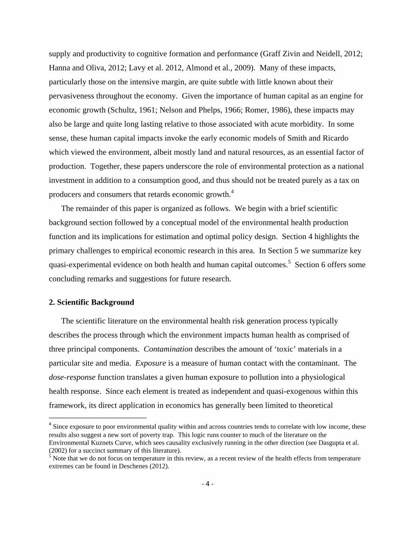
Figure 1 shows air pollution levels over time for China, Mexico, and one city in the US,
Pittsburgh, focusing on particulate matter less than 10 microns in diameter (PM10).18 Several
features of this Figure are noteworthy. First, since developed countries began monitoring
environmental quality earlier than their developing country counterparts and are more likely to
place that data in the public domain, we can construct a longer time series for the U.S. than for
Mexico or China.19 Second, air pollution has improved tremendously over time in all 3
countries, regardless of development status. Levels in Pittsburgh dropped by over 80% since
1950 and 40% since 1990, and levels in both China and Mexico have fallen by roughly 50%
since 1990. Third, although pollution levels in China and Mexico are always higher than levels
in the US at the same point in time, the levels experienced in those countries today are not unlike
historical levels in the U.S. Contemporary pollution levels in China and Mexico are similar to
those found in Pittsburgh in the mid-1970s and mid-1990s, respectively. As such, studies based
on historical pollution levels in the U.S. may also be informative about current health and human
capital impacts in developing countries.
Acquiring time-stamped health data with geographic identifiers that permit the merging
of environmental data is an additional challenge, regardless of country development status.
Health surveys often contain limited geographic identifiers in order to protect subject
confidentiality, although increased access to non-pubic versions via various Research Data
Centers has eased this constraint.20 Various health censuses, such as birth and death records
17 In addition to the limited scope of pollutants for which remote sensing is feasible, other problems include poor spatial resolution, the inability to distinguish surface from upper atmospheric pollution, and the interference cloud cover causes in obtaining reliable estimates. 18 We focus on PM10, rather than PM2.5, because of data availability. We also focus on Pittsburgh because of the availability of a particularly long time series (Davidson, 2000; Rawski 2006); values for Pittsburgh are, however, quite close to the average across all major cities. Since PM10 has only been measured more recently, older values of PM10 are obtained by multiplying measures of Total Suspended Particles (TSP) by 0.55. A complete time series for TSP was imputed using data on dust fall. We thank Thomas Rawski for generously sharing this data, originally obtained from Cliff Davidson. 19 While reported pollution levels in China may be subject to manipulation, evidence also indicates that reported pollution levels are highly correlated with data from independent sources (Chen et al., 2013). 20 Although access to non-public versions of these health surveys offer promise, it is important to keep in mind that such data were not designed to be used for spatial analyses. For example, the National Health and Nutrition
‐ 15 ‐
stored in Vital Records and Hospital Discharge Data, often provide easier access to geographic
identifiers as well as the exact date of the birth, death, or hospital admission. As we describe in
the following section, several studies have acquired administrative data sets with detailed
geographic identifiers to more precisely assign pollution exposure.
Once environmental and the relevant outcome data sets are identified, merging them is a
non-trivial exercise as well. It requires important assumptions about individual mobility and the
spatial distribution of pollution, which is often non-uniform even over relatively small spatial
scales. For example, the New York City Community Air Survey (NYCCAS), a unique project
launched by both the city and academic institutions within the city, found that differences in
building heating oils, proximity to traffic, and vegetative cover lead to considerable variation in
particulate matter contamination in the air across closely located city blocks (Clougherty et al.,
2009).
4.B. Measuring pollution
i. Assigning pollution to individuals Given the geographic information contained in large scale data sets, studies often
approximate contemporaneous pollution levels based on an individual’s general location and the
location of the monitor. This crude approach leads to measurement error that increases with an
individual’s distance from the monitor and the degree to which pollutants disperse non-
uniformly. This measurement error will typically bias estimates downward, but with a large
enough dataset researchers can use data from multiple monitors, various weighting techniques,
and factors that affect the dispersion of pollution to obtain more precise assignments of localized
pollution.21 A finer level of geographic disaggregation for individuals, such as a residential
address, also allows for better assignment of relevant pollution levels and hence is more likely to
provide precise estimates.
The usual mobility of individuals throughout their life (i.e., not as a form of avoidance
behavior in response to pollution, which we discuss below in 4C), both within a day and over Examination Survey (NHANES) only samples from a small number of counties in order to keep survey costs down, which greatly limits spatial variability. 21 Such methods include inverse distance weighted average (Currie and Neidell, 2005), kriging (Lleras-Muney, 2010), and land-use regression (Jerret et al. 2005).
‐ 16 ‐
time, can also present a challenge for assigning potential exposure. On a daily basis, individuals
spend their time not only at home but at work, school, and other possible locations that are not
typically recorded. Although the use of personal monitors attests to this mobility (Tonne et al.,
2004), two issues remain: 1) the high costs of personal monitoring often result in the use of a
small, unrepresentative sample without a clearly defined control group; and 2) the link to policy
is less clear because indoor sources also contribute to pollution, making it difficult to pin down
the sources of pollution and the scope for regulation. Mobility over time also presents a
significant measurement challenge in assigning cumulative exposure over longer periods of time.
Focusing on children, and in particular infants, whose shorter life span has permitted less
mobility, can greatly limit this concern (Joyce et al., 1988; Chay and Greenstone, 2003a).
Clearly, this comes at a cost since studies of children may not tell us much about impacts on
alternative populations of interest, such as the elderly or those with respiratory problems.
Instrumental variables offers one approach for combating "classical" measurement error in
pollution, and below we describe several instruments that have been used in the literature.
ii. Functional form of pollution Early epidemiological investigations on the health effects of pollution predominantly
focused on extreme pollution events, with one of the most famous being the “killer fog” in
London, England in December, 1952 (Logan and Glasg, 1953). A temperature inversion
combined with windless conditions led to a sudden and dramatic increase in air pollution. Since
residents were used to winter fogs, there were little, if any, changes in behavior, leading to a
rather clean measure of pollution impacts in this case. The dramatic rise in mortality that
precisely coincided with the timing of the fog, along with results from studies with similar
research designs (e.g. Townsend, 1950; Firket, 1936; Greenburg, 1962), have produced
compelling evidence that high levels of pollution pose a significant threat to human health.
While high pollution levels may be relevant in developing countries, these extremes are
dramatically higher than those faced by nearly all people in developed countries today (refer to
Figure 1). This is important because the processing of pollutants by the human body is subject to
a number of rate-limiting steps that imply non-linear health effects that have been widely
supported by laboratory studies in the toxicology literature (e.g. Lefohn et al., 2010; Smith and
‐ 17 ‐
Peel, 2010). Indeed, thresholds below which no harmful effects are observed have been found
for some pollutants (Stoeger et al., 2006; Pottenger et al., 2009), raising serious concerns about
extrapolating health effects from high pollution levels to low ones.
As such, interest has largely shifted to understanding the health effects from more modest
pollution levels, with an emphasis on identifying ‘safe’ levels below which pollutants have no
meaningful health effects. This shift in emphasis to the lower-end of the pollution distribution,
however, makes the choice of study outcomes particularly important. It may be that mortality or
hospital admissions are only induced when pollution exceeds a certain threshold, while more
subtle forms of morbidity and impairment arise at lower levels. Our limited understanding of the
human capital and productivity effects of pollution at any level, however, underscore the
importance of studies throughout the pollution level spectrum in order to better explore the full
range of impacts in this emerging area of importance.
To explore possible non-linear effects, the most widely used approach is to discretize
pollution levels through the use of dummy variables, which can be specified in several ways.
One approach is to specify thresholds based on government standards, which helps to relate
estimates directly to policy. For example, Currie et al. (2009a) include a series of dummy
variables for pollutants as they relate to National Ambient Air Quality Standards. Another
approach is to use laboratory evidence on thresholds, though measurement error in assigning
pollution may limit its effectiveness. The most flexible but also data demanding approach is to
define pollution as a series of dummy variables, with somewhat arbitrarily chosen knots. This
approach is akin to a nonparametric regression with a uniform kernel and no overlap; unlike non-
parametric regression it can be estimated in an ordinary least squares framework, and is therefore
amenable to a wide range of econometric tools for causal inference.
iii. Duration of exposure
Specifying the appropriate duration of exposure is also important. Some pollutants have a
nearly immediate effect – exposure to ozone can inflict symptoms in as quickly as 1-2 hours –
while some have a longer incubation period. Even more complicated, some have both immediate
and delayed effects. Since we may not know which period of exposure is most important a priori,
this is largely an empirical question. A distributed lag specification, which allows for both
‐ 18 ‐
contemporaneous and lagged exposure, allows for a flexible duration. Correlations in pollution
values over short periods of time, however, can lead to multi-collinearity, hampering our ability
to precisely identify the coefficients for specific time periods. A joint F-test of all time periods
enables one to obtain an overall understanding of the relationship between multi-day exposure
and outcomes without distinguishing between individual days. The precise temporal pattern of
impacts is generally unimportant for policy, which typically uses rather blunt instruments to limit
contamination and exposure at a broad level rather than on specific days. .
For examining long run effects, analyses become increasingly complicated, particularly
for understanding the impacts from cumulative exposure over a lifetime. In addition to individual
mobility over time hampering the assignment of cumulative exposure, specifying the proper
functional form for this relationship is a major obstacle. Accounting for the other behaviors over
one’s lifetime that affect health and thus potentially confound this relationship is equally
challenging. In Section 5 we discuss quasi-experimental evidence on long-run effects that arise
due to a latent response to an acute exposure in the distant past, but we are unaware of any quasi-
experimental evidence on the cumulative effects of pollution exposure.22
When focusing on birth outcomes, an area of intellectual inquiry that has grown
tremendously in recent years, the relevant period of exposure is also important, albeit more from
a developmental perspective than an environmental policy one (Salam et al., 2005). For instance,
the first trimester is the period during which the neural tube is transformed into the brain and
spinal cord and many other organs experience rapid development (de Graaf-Peters and Hadders-
Algra, 2006; Cunningham et al., 2010), making this a particularly vulnerable stage in terms of
environmental insults. One complication when parsing exposure by trimester of pregnancy is that
length of gestation can be affected by pollution, making the definition of each trimester, and thus
the total in utero exposure, endogenous (Currie et al., 2013). More challenging, however, is that
including multiple trimesters of pollution simultaneously can lead to severe multi-collinearity,
sometimes resulting in seemingly beneficial effects from pollution in certain exposure periods.
4.C. Endogeneity of pollution
22 For recent evidence on the association between cumulative exposure to pollution over several years and health, see Janes et al. (2007), Pope et al. (2002), Jerrett et al. (2009), Rojas-Martinez et al. (2007), and Miller et al. (2007).
‐ 19 ‐
Early research on the health impacts of pollution took a rather fatalistic approach –
people (and thus markets) are unaware of ambient pollution levels such that once it is in the air
nothing can be done about it. As knowledge about pollution has grown, both in terms of our
ability to detect it and to understand its health effects, the fallacy of this original assessment has
become clear. Pollution exposure can be altered in a variety of ways, making it an endogenous
variable with all of the usual concerns that come with it. Recognizing these sources of
endogeneity has led to the use of quasi-experimental research designs that effectively eliminate
(or significantly reduce) this problem.
i. Residential sorting
The major driver of endogeneity is residential sorting: individuals choose residential
locations based on the attributes of that area, which leads to a non-random assignment of
pollution. Preferences over residential neighborhoods depend on the employment opportunities,
commuting costs, and local amenities in the area (Tiebout, 1956; Roback, 1982), where local
amenities include elements such as school quality, parks, housing stock, crime, hospitals, and
environmental quality.23 Importantly, these amenities are bundled such that environmental
quality is packaged with other attributes in a location, although the specific contents of a
particular bundle vary by location. For example, urban areas may have worse air quality but
better schools than rural areas, while suburban areas may have both better air quality and schools
than inner cities. The key point is that optimizing individuals make tradeoffs along multiple
dimensions based on the intensity of their preferences for each local attribute, which implies that
the characteristics of the neighborhood in which individuals live, including pollution levels, are
endogenously determined.24
Different levels of exposure due to sorting can be driven by three factors. The first is
heterogeneity in preferences over local amenities. Since these local amenities are often correlates
23 For simplicity, we assume preferences over environmental quality solely because of health benefits, but the same basic intuition holds if we extend this to include preferences over environmental quality because of visibility or odor. 24 Of course, an individual’s ability to trade off attributes will be a function of prices, which depend on aggregate preferences over attributes and thus market demand for and supply of housing in a given location (see, for example, Bayer et al., 2010). For an explicit ‘test’ of the Tiebout mechanism in an environmental context, see Banzhaf and Walsh, 2008).
‐ 20 ‐
of air quality, we can view them as indirect preferences over air quality. The second is income. If
local amenities are normal goods, then wealthier people will live in areas with better local
amenities, which can affect air quality to the extent that it is correlated with other amenities. The
third is heterogeneity in susceptibility to pollution. In this case, we view sorting as a direct result
of preferences over air quality.
The importance of highlighting these three factors is that they have different implications
for cross-sectional estimates of the relationship between pollution and health/human capital. The
former two factors lead to omitted variable bias. Wealthier individuals might live in
neighborhoods with better air quality (driven by preferences for local amenities correlated with
air quality), and they also are likely to make other investments in their health that are difficult to
observe; this would bias estimates down. On the other hand, people who live in or near cities
face worse levels of air quality but could have access to better quality health care and jobs that
improve health; this would bias estimates up. Clearly, the overall direction of bias introduced by
this sort of endogeneity is theoretically ambiguous.
In contrast, residential sorting due to direct preferences for cleaner air can lead to a
simultaneity bias. If susceptible people relocate to less polluted areas to reduce the onset of
symptoms, then health is affecting one's pollution exposure. To fix ideas, imagine an extreme
case where there are two types of individuals, non-asthmatics and asthmatics. Pollution causes
asthmatics to have hospital admissions, but not non-asthmatics. Initially, individuals are evenly
distributed across a "dirty" area and a "clean" area. If the asthmatics relocate to the clean area to
reduce clinical symptoms induced by pollution, the average health stock in the clean area will
decrease while the health stock in the dirty area will improve. If this sorting were not recognized,
it would look as if pollution actually improved health. Although the stylized nature of this
extreme case is unrealistic, it underscores one important mechanism through which sorting may
hinder inference.
Table 1 illustrates the sorting problem. Data for this Table are from the 2001-2006 waves
of Behavioral Risk Factor Surveillance System (BRFSS).25 We focus on these 6 years because it
already includes merged air pollution data at the MSA level; a rather crude measure but one that
is still sufficient for illustrating our point. In each row, we present the mean and the coefficient 25 For more details on the BRFSS, see http://www.cdc.gov/Brfss/.
‐ 21 ‐
of each variable, where the coefficient is obtained by regressing each variable on the Air Quality
Index (AQI) – a summary measure of air quality across several pollutants -- and dummies for
each survey wave. For example, the first row shows that roughly 77 percent of respondents have
participated in some form of exercise in the past month. The estimate of -0.118 implies that for
each 10 unit increase in the AQI, there is an 11.8 percentage point drop in the rate of exercise.
Consistent with sorting, we see that respondents of higher socioeconomic status and those with
higher levels of health investments generally live in neighborhoods with better air quality,
though not necessarily in a monotonic pattern. This underscores the non-random assignment of
pollution levels. While it is possible to control for these factors, it is unclear whether one can
adequately control for all relevant factors, highlighting the potential for bias under cross-
sectional approaches.
Although a complicated and seemingly insurmountable empirical challenge, the main
approach for tackling sorting is to find "shocks" to air quality that push the market temporarily
out of equilibrium, often accompanied by fixed effects that hold other characteristics of the area
constant. These shocks can be driven by air quality regulations, abrupt changes in industrial
production (such as strikes and plant closings), or catastrophic events (such as temperature
inversions or wildfires). Finding such shocks presents a major obstacle, and it is not surprising
that many of the same shocks are used across studies. Controlling for other major changes that
may accompany a shock is also a challenge. For example, a plant closing that lowers pollution
might lead to disruptions in income and health insurance that could also impact health and
human capital.
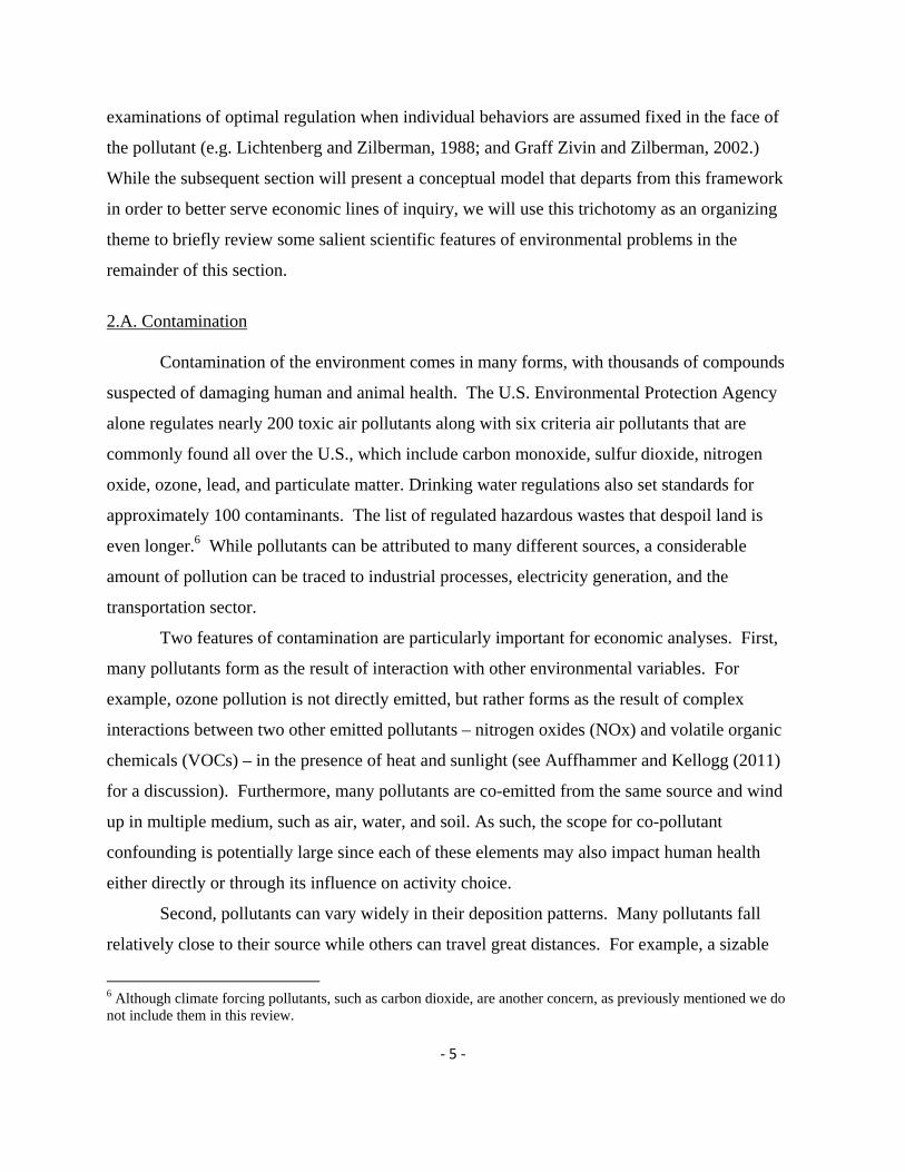
Since many pollutants exhibit a high level of variability from one day to the next, high
frequency variation in pollution can also be exploited to address sorting.26 Figure 2 provides a
glimpse of this for ozone. The first panel plots demeaned, daily ozone levels for a downtown Los
Angeles, CA monitor for June-September, 2010. Immediately evident, ozone swings from one
day to the next are substantial, often nearly as large as the overall mean level of ozone of 0.043
parts per million (ppm). Focusing on such short-run variation, however, requires careful
consideration of what causes the higher frequency changes in pollution levels to ensure they are
26 Of course individuals can modify their activities (and the location of activities) in response to these daily fluctuations, a point we return to in the next subsection.
‐ 22 ‐
not driven by local activities that might also affect health and human capital. In the case of
ozone, this variation is due to weather, regional transport of ozone and its precursors, and the
highly nonlinear ozone formation process. Since weather is an important confounder, the second
panel of Figure 2 plots the residuals from a regression of ozone against several weather variables
(along with day of week dummies), and the variation is only minimally dampened, providing
additional support to the notion that daily variation can be viewed as plausibly exogenous.
One concern with using such high frequency variation, however, is that daily changes in
pollution may be less informative about possible impacts from new regulations, which lead to
more permanent shifts in pollution. A second concern, and one that only arises when examining
mortality impacts, is short-term mortality displacement, commonly referred to as “harvesting.”
Mortality for an otherwise healthy individual represents a significant loss to society, but
mortality for an already ill person, whereby pollution serves to hasten the death by a few days or
weeks, presumably imposes less social cost. While an offered solution is to assess the degree to
which estimates change when aggregating to a lower frequency, this is an imperfect solution
because it shifts away from the underlying premise of this approach.
To illustrate the value of exploiting plausibly exogenous changes in pollution, we present
some basic estimation results in Table 2 using the same BRFSS sample. We approximate a
‘shock’ by including MSA fixed effects -- an admittedly imperfect quasi-experiment that exploits
the natural year-to-year fluctuations in pollution, but one that again illustrates our principal point.
The first panel focuses on tooth loss as a dependent variable. Tooth loss should not be affected
by air pollution, so evidence to the contrary suggests model misspecification.27 The first three
columns present cross-sectional estimates and the last three fixed effects estimates, with a
gradual increase in controls within each model as we move rightward. The estimate in column
(1) implies that a 10 unit increase in the AQI leads to a 6.3 percentage point increase in having
lost any teeth, which represents a 13% increase from the mean. The result becomes somewhat
smaller as we add more controls, but remains statistically significant at conventional levels,
supporting the surprising conclusion that air pollution makes one's teeth fall out. A more likely
explanation is that oral health is the result of an accumulation of unobserved investments in
27 While pollution could indirectly affects tooth loss through interactions with comorbidities over long time periods, the gradual nature of tooth loss implies it will be insensitive to a short term change in pollution.
‐ 23 ‐
health, and people living in more polluted areas have lower levels of investment. In support of
this, when we include fixed effects to capture time invariant characteristics of MSAs, this odd
finding disappears, shown in columns (4)-(6). These results illustrate the importance of fixed
effects even when a rich set of controls are available.
Since fixed effects over such a short time frame may have the unintended consequence of
removing too much of the variation in pollution, we continue this example focusing on two self-
reported outcomes plausibly affected by pollution. The first is the number of days in the past
month with bad physical health (panel 2), which can be viewed as a measure of illness (φ). The
second focuses on self-reported general health status (panel 3), a measure of health capital (H).
Repeating the same set of regressions, cross-sectional estimates for days of bad health are
statistically insignificant and quite unstable; the addition of a handful of behavioral factors
(exercise, smoking, and whether one had the flu shot) halves the estimate. The fixed effect
estimates, however, are much more stable, considerably larger in magnitude and statistically
significant, suggesting ample variation across years for detecting changes in health flows. The
estimate of 1.225 from the last column implies a 10 unit increase in AQI increases bad health
days by over a third. Since health status has less variation than illness, we do not find a
statistically significant relationship between AQI and being in poor, fair, or good health in any
specification. While this table highlights the potential strength from using fixed effects, it also
demonstrates the caution needed in interpreting results across dependent variables that arise from
different processes, a point we discuss in more detail below in 4D.
ii. Environmental confounding
In addition to optimizing behavior causing endogenous pollution exposure, omitted
variable bias may also arise from concurrent changes in the environment. Of particular concern
is weather. As previously mentioned, weather interacts with some types of emissions to form
pollution. Weather may also have a direct impact on health (Deschenes and Greenstone, 2011),
making it a potentially important confounder. Since weather is typically observable at the same
or finer scale than pollution data, this challenge can be obviated through the careful control of
relevant variables. As with pollution, the functional form of weather must be carefully
considered.
‐ 24 ‐
Environmental confounding can also occur because the emissions of many pollutants are
highly correlated. Many air pollutants, especially in urban areas, are co-emitted. For instance,
automobiles emit particulate matter, carbon monoxide, and contribute to ozone pollution.
Similarly, industrial mix and geography can create pollution hot spots, with high levels of toxics
in air, water, and soil. As with meteorology, the careful selection of controls is essential and thus
requires an understanding of both the pollution generation process and its likely impacts. For
example, nitrogen dioxide leads to the formation of ozone, but may also have direct health
effects; controlling for it may unnecessarily dampen estimates of the impact of ozone pollution
on health and human capital, but not controlling for it may overstate the impact.
The fact that many pollutants can be traced back to the same emission source introduces a
complication for instrumental variable (IV) approaches. A single shock to an emission source,
such as a plant closure or unexpected changes in boat or vehicle traffic, can affect multiple
pollutants simultaneously, making the model unidentified without further assumptions. Since
meteorological conditions, such as wind speed and direction, interact with emissions to impact
pollution formation and deposition, knowledge of this process can be incorporated to aid in
identifying the effects of multiple pollutants. However, weather is also an important confounder
in its own right, necessitating additional assumptions regarding the functional form of the
relationship between health, pollution, and meteorological conditions in order for this to improve
identification. See, for example, Schlenker and Walker (2011) and Knittel et al. (2011), for
applications along these lines. Reduced form relationships focusing on the source of emissions,
rather than pollutants per se, may be estimated to circumvent this issue.
iii. Avoidance behavior
Another source of endogeneity stems from avoidance behavior – transient actions
individuals deliberately take to reduce their realized exposure to pollution.28 For example, on a
high ozone day, spending less time outside or shifting outdoor activities towards twilight hours is
28 Although residential sorting with respect to preferences for clean air can be viewed as a form of avoidance behavior, we distinguish it from this more temporary avoidance behavior because failing to account for the two different types of avoidance behavior have different implications for estimates, as elaborated below. A similar logic applies to more permanent actions designed to limit exposure to pollution, such as home air or water filters that run constantly once purchased.
‐ 25 ‐
a highly effective means for reducing exposure. Such short-run responses require knowledge
about daily and even hourly pollution levels. Certain pollutants are observable at high levels of
concentration, thereby facilitating avoidance. Others are correlated with observable phenomenon
and thus can be inferred, e.g. the proliferation of face masks in many Asian cities is in response
to an observed haze that is indicative of ozone and fine particulate matter pollution. When
pollution levels are more modest and thus less easily discernible by the citizenry, direct
observation has largely been replaced by air quality alerts and other public information
campaigns. The most susceptible individuals can also independently monitor their lung
functioning to approximate their sensitivity on any given day, indicating a role for private
information in avoidance behavior as well. In the end, the degree to which such short-run
behavioral responses will be important depends upon the ‘visibility’ of pollution, either literally,
through information dissemination, or through health feedbacks that allow individuals to infer it
based on physiological responses.
Unlike sorting, which affects the ambient levels of pollution where an individual resides,
avoidance behavior is a response to ambient levels. That is, avoidance behavior occurs after an
individual learns the ambient pollution level (a “post-treatment” variable). As such, including or
excluding avoidance behavior does not introduce a bias per se, but affects the interpretation of
estimates. For example, if focusing on hospital admissions, directly controlling for avoidance
behavior yields estimates of the biological effect (δφ/δP), while omitting it yields estimates of
the reduced-form effect (dφ/dP).
Moreover, the scope for short-run avoidance behavior complicates the use of shocks to
identify the effect of pollution. When a shock leads to an abrupt change in pollution that is
unobservable by the populace, behavioral responses are not feasible and the shock can be used to
derive a measure of the biological impacts of pollution. However, when a shock is more gradual
(such that information about pollution can be publicly disseminated), or individuals can directly
observe the change (possibly because a pollutant or its correlates are visible), the shock does not
obviate the need to account for avoidance behavior. Clearly the degree to which shocks allow
potential time-varying behavioral responses to changes in pollution levels will vary across
settings depending on the availability of this public and private information.
‐ 26 ‐
The question then becomes, should one control for avoidance behavior? The reduced
form is generally more convenient for valuation, described in more detail below in 4E, because
the econometrician does not need to specify the functional form of the environmental health
production function with respect to P and A. This is particularly helpful since data limitations
often necessitate the use of proxy or incomplete measures for avoidance behavior. The pure
biological effect may be of interest to economists for its generalizability, at least across settings
that are relatively homogenous in terms of age composition and underlying health.29 Avoidance
behavior is clearly very context specific, even within the same population over time (Graff Zivin
and Neidell, 2009), so reduced form estimates are likely to vary across settings. Furthermore, it
is important to know the biological effect in order to design policies to encourage avoidance
behavior. Ideally, one would estimate both the biological and reduced form effects, with the
difference reflecting the benefits from avoidance behavior -- δφ/δA*δA/δP (or δH/δA* δA/δP).
When avoidance behavior is precipitated by the provision of information, this difference then
reflects the value of the information provided.
4.D. Outcome measurement
Pollution can have myriad health effects and a simultaneous accounting of all of them is
essential for welfare calculations and the design of optimal policy. For example, a high pollution
concentration may cause an individual to use more medication, visit the ER, and then, ultimately,
to die prematurely. Many additional impacts may occur that are not captured by health
encounters. Data limitations require all studies to paint a partial picture, which can often be
considered a lower bound of the full effects. Yet, taken as a whole, economists have examined a
wide range of outcomes that result from an equally varied set of quasi-experiments. These
results have deepened our understanding of which impacts are economically significant.
Moreover, by bounding impacts they may help us determine threshold rules for policy whereby
regulatory action is taken when a subset of the benefits exceed the costs.
29 While toxicologists should have a comparative advantage in measuring the pure biological effect through the use of chamber studies, as previously mentioned the endpoints used in these laboratory settings are often of limited value for policy design since they are frequently designed solely to understand the mechanisms of action. This leaves ample room for learning about the biological effects in a non-experimental setting by controlling for avoidance behavior.
‐ 27 ‐
In the discussion that follows, we group health outcomes as they relate to equation (9).
The first distinction we make is between health capital (H) and illness (φ), where health capital
can be thought of as a stock measure and illness as a flow that draws down that stock, at least
until medical treatment is completed or the disease has run its self-limited course. The second
and perhaps more novel distinction is to separate between classes of illnesses. Some illnesses
lead to health encounters, such as hospital admissions, doctor visits, and medication use. These
highly visible encounters end up in standard health data sets, and as such are readily observable
by the econometrician.
The other class of illnesses is more subtle and while it may not result in any formal health
encounters (δM/δφ = 0), it nonetheless leaves a ‘signature’ of impacts. For example, pollution
may cause an individual to feel minor discomfort, irritation, or labored breathing, not unlike that
from cold or seasonal allergies. This does not prevent them from participating in usual activities,
but affects performance conditional on participating – a distinction between the extensive and
intensive margin we will return to later. Alternatively, a fetus exposed to pollution may
experience physiological changes that result in lifelong impacts, but such changes may be latent
and not readily detectable and treatable at birth. Although these effects are more subtle, they
may be more pervasive, suggesting potentially large welfare effects. We maintain this
distinction here since the absence of a health encounter that can be directly associated with
pollution exposure makes them particularly difficult for the econometrician to observe.30
i. Health capital
Since health is a complicated construct often influenced by subjective interpretations,
there is unfortunately a rather limited set of reliable measures of health capital available.31 One
of the most commonly used measures in environmental and health research is mortality. As
quite possibly the most objective measure of health, it serves as a useful benchmark for making
comparisons across large spatial and temporal scales. Furthermore, since it typically comes from
30 It is worth noting that the lack of a health encounter may arise for at least three distinct reasons: 1) effective treatments are unavailable; 2) symptoms are minor enough that they do not necessitate the use of formal care; or 3) symptoms are sufficiently subtle that they are not ‘observed’ by the individual experiencing them. 31 Despite our use of self-reported health status in Table 2, reliability concerns with self-reported data of this nature have limited their use in the environmental economics literature.
‐ 28 ‐
vital records maintained by governmental agencies, it often captures a census of deaths,
permitting large samples for analysis. Reasonably detailed geographic identifiers, such as the
county of residence, are also routinely available, facilitating the assignment of pollution to
individuals. In the context of our conceptual model, it is useful to define mortality as health
stock falling below a certain threshold (H<h*). In that case, researchers typically estimate dH/dP
as defined in equation (9).32
Birth outcomes, such as birth weight, gestation, and APGAR scores, are another desirable
measure of health capital, albeit for a select population. Since a fetus goes through rapid
development in a short period of time, understanding the effects of pollution on this group are
particularly important. Birth outcomes have been linked with both higher healthcare costs at birth
and later in life (Almond et al., 2005; Currie and Hyson, 1999). Since these data generally come
from vital records, they share many of the desirable properties of mortality data (large samples,
date of event, and detailed geographic information). Since pollution may affect both conception
(Buck Louis et al., 2009) and fetal deaths (Sanders and Stoecker, 2011), focusing on birth
outcomes also introduces a potential concern regarding the endogeneity of births.
While these outcomes measure specific aspects of health, it is also important to recall that
health is affected by how illness episodes are treated, as discussed in the conceptual framework.
This link between health and illness suggests that health capital will show less variation than
illness, which can greatly influence statistical inference. For example, pollution may induce a
large increase in hospital admissions for myocardial infarctions (i.e., heart attacks), but a
considerably smaller change in mortality because major medical advances have significantly
improved survival rates (Cutler et al., 2006). A study only focusing on mortality may fail to
uncover this relationship; this is precisely the pattern found in Table 2, which focused on self-
reported health status and daily episodes of compromised physical health. Since this link
between health and illness also varies with technology and access to high-quality health care,
32 Note that these studies seldom employ controls for medical treatment (M) that may have preceded death. For example, if particulate matter induces a death from a heart attack, that individual likely received hospital treatment for their cardiovascular complications before passing. These expenditures are often not considered because mortality and hospitalization data come from distinct sources that are not linked. Since the value of a statistical life (VSL), which is often used to monetize these impacts, does not include end of life spending, estimates of willingness-to-pay to reduce pollution based solely on VSL will miss this component, though they may be small relative to the VSL.
‐ 29 ‐
estimates of the relationship between pollution and health may vary considerably over time and
across space.
ii. Illness
In addition to measuring impacts on health capital, research often focuses on the impact
of pollution on illness (φ). Throughout, we use the term illness to broadly refer to any
underlying physiological impact, some of which may be readily treatable through medical
interventions while others may be less conducive to medical management.
ii.a. Observable illnesses
The vast majority of studies that examine illness endpoints rely on health encounters as
their data source. Illnesses that result in hospital and emergency department (ED) visits have
been the bread and butter of epidemiological studies, and a common focus in economics as well.
The appeal of such outcomes lies in the quality and quantity of data: these visits come from
administrative hospital files, form a census of patients, rely on the standard "International
Classification of Diseases" to identify specific health conditions, contain the date of discharge,
and provide detailed geographic residence, such as the ZIP code of the patient, that allows this
information to be merged with pollution data.33
Despite the significant appeal, using these visits may introduce sample selection bias.
Those who have a relationship with a primary care physician (PCP) may receive routine or
preventative care so that they never experience a hospitalization; access to a PCP is clearly
endogenous. To illustrate, imagine two areas where pollution has biologically-equivalent effects
on people and increases identically over time, but the areas differ in terms of access to PCPs.
The high access area may experience little change in hospitalizations, while the low access area
may witness significant increases. Since access to non-hospital-based healthcare is often highly
correlated with other determinants of health (Institute of Medicine, 2002), this introduces a non-
33 The exact date of discharge and patient ZIP code is typically only available in non-public versions of the data, which often requires some form of human subjects review.
‐ 30 ‐
random selection of data for analysis.34 Administrative data from countries with more universal
access to healthcare can help overcome this challenge when all forms of care are reported.
Hospital data can also be used to calculate medical expenditures. Medical expenditure
data has two advantages: it is already monetized and it can reflect the severity of disease. For
example, some hospital admissions for respiratory difficulties are relatively minor events that are
remedied by the use of quick-relief inhalers and steroids, while others can be life threatening and
require the use of infusions and ventilators. Hospital charges will differ across the two types of
admissions and thus serve as an indicator of disease severity.35 The validity of this construct will
depend, in part, on the marginal productivity of medical care (δH/δM) for each of the two disease
types since health at discharge is an important component of impacts. Since this approach also
involves use of the admissions data, the same strengths and limitations described above apply.
Increases in the availability of emergency room data in the US can lessen selection bias concerns
by capturing the universe of individuals seeking hospital-based care, including individuals who
may use the emergency room as a source of primary care.
Medical care expenditures can also be assessed based on sales of medications.
Asthmatics, for example, often take both controller medications on a routine basis and quick-
relief medications to relieve symptoms as they arise. Hence, the use of quick-relief medications
provides a unique opportunity to examine more subtle health effects that may not be captured in
the use of health care services. Since recovery using these inhalers is generally quite rapid,
medication expenditures likely capture most of the pollution-induced costs associated with that
particular exposure episode. Despite this potential advantage, storability of these medications --
quick-relief asthma inhalers can deliver hundreds of "puffs" -- may lead to little variation in
purchases over short time periods. Obtaining such data is also complicated by the fact that it is
often the proprietary information of retailers. Through individual agreements, researchers can
sometimes obtain data on store-level sales. Some agencies, such as IMS Health, obtain and
aggregate data from multiple retailers, though such data is often only available at a significant
34 In principle researchers could focus directly on physician visits as another measure of illness, but obtaining this data with suitable geographic identifiers is a significant challenge. Moreover, sample selection bias remains a concern, unless used in conjunction with data on substitute encounters, e.g. emergency room and pharmacy visits, for the same sample. 35 Note, however, that many studies that use hospital admissions value the pollution effects using average hospital charges, which does not capture severity.
‐ 31 ‐
price. Even with store-level sales data, assigning pollution to those sales can be tricky as the
transaction location may differ from the location where exposure took place, e.g. exposure may
be at work while one may use a pharmacy near their home. Given these limitations, medication
data has seldom been used in the environmental economics literature, though Deschenes et al.
(2012) are an important exception.
It is worth noting that illness encounters are typically viewed as indicative of illness, but
they also represent ameliorative actions. Therefore, how these illnesses translate into health
impacts vis-à-vis our conceptual model is governed by the demand for health care (δM/δφ) and
its effectiveness (δH/δM). Both are areas of major preoccupation within the field of health
economics (e.g., Manning et al., 1987; Finkelstein et al., 2011; Card et al., 2009; Cutler, 2007;
Lichtenberg, 2007). When combined they reveal the transient and perhaps residual, untreatable
health effects due to pollution (as implied by δH/δφ). To be concrete, imagine a patient that is
hospitalized with an acute cardiac condition. The relevant health measure would not describe the
patient’s health condition at admission but rather the one at discharge. In practice, this complete
accounting is rarely done.
ii.b. Unobservable illnesses
While the aforementioned measures of illness are relatively straightforward to observe,
health can be impacted in more subtle ways that do not generate health encounters of any sort.
These ‘unobservable’ effects from exposure can begin with symptoms such as eye, ear, nose, and
throat irritation, and may manifest themselves in labored breathing, increased fatigue, and lack of
focus, all of which create disutility and can affect performance at work or in school. They also
include changes in human development, which are particularly important for understanding the
impact of early life exposures. Given the difficulty in observing these impacts, the emerging
economic research in this area focuses on proximate outcomes, such as worker productivity,
student test scores, and birth outcomes. Of course, such outcomes are also of direct interest to
economists as human capital has long been viewed as an engine for economic growth (Schultz,
1961; Nelson and Phelps, 1966; Romer, 1986).
In medical and epidemiological fields, there is a long history of using surrogate health
outcomes that are predictive of an endpoint of interest, such as forced expiratory volume,
‐ 32 ‐
microvascular function, and blood pressure (e.g., Hazucha et al., 2003; Pope et al., 2011).36
These surrogate measures capture subtle changes in physiologic function that do not result in
medical treatment, and may even be unobserved by the individual. Nonetheless, these subclinical
changes may have impacts on mental and physical functioning that impair learning and job
performance, providing a strong rationale for human capital and productivity impacts.37
The biggest challenge to research in this area is finding suitable sources of data. An
emerging body of economic research focuses on the manifestation of these subtle effects as
captured by outcomes at school or the workplace, principally absenteeism and performance. The
use of such data does not involve sample selection since outcomes are not only measured for the
sick but for all. They are also generally straightforward to monetize, as test scores and
performance can be readily linked with wages – a rich area of study in the labor and education
fields (Black et al., 2007; Currie and Thomas, 2001; Oreopolous et al., 2008; Royer, 2009) – and
thus directly inform our understanding of δw/δH*δH/δP.38 Limited data availability, especially
for representative samples, is, however, a formidable obstacle to the conduct of credible
empirical work in this area.
4.E. Valuation
A common goal of environmental economics research is to take estimates of the
environmental-health relationships to develop measures of willingness-to-pay for reductions in
pollution, as specified in equation (10), in order to inform the design of optimal environmental
policy.39 To obtain the welfare impacts from a change in environmental quality, one would want
to measure all of the aforementioned health impacts. For example, particulate matter pollution
36 The primary reason for the focus on surrogate measures is that it is often the only ethical way to conduct a chamber study (i.e., randomized experiment) without inducing disease. 37 Such impacts are also consistent with the large economic literature that has found linkages between health, education, and labor market outcomes. See, for example, Strauss and Thomas (1998). 38 Since these effects are more subtle, there are often limited opportunities for avoidance behavior (δA/δP=0) and medical consumption (δM/δP=0). As such, the biological and reduced-form effects on health will be identical (δH/δP = dH/dP). 39 Several alternative approaches for valuing environmental quality exist, including the hedonic pricing method, contingent valuation, and the travel cost method. For a detailed review of these valuation approaches, see Braden and Kolstad (1991).
‐ 33 ‐
may affect mortality, hospitalizations, medication use, and productivity, so one would want to
sum up all components, being sure not to double count.40
In addition to measuring all of these components, one must also place a monetary value
on each, and all are not without controversies. With the exception of mortality, which is
monetized by using the value of a statistical life (VSL), all valuations likely understate the true
economic costs.41 Charges are typically the only measure available for hospital admissions, and
they do not capture the costs associated with the pain and suffering experienced by sickened
individuals or their family members.42 The use of medications as an outcome provides a clean,
direct measure in dollars, but it does not account for possible side effects from medication use
(e.g., routine use of inhalers may cause arrhythmias (Singh et al., 2011)). Changes in birth
outcomes can be linked with future earnings (Black et al., 2007; Royer, 2009), but this does not
include the disutility or medical expenditures due to health effects later in life.
In addition to these direct health impacts, avoidance behavior should also be included
when valuing demand for environmental quality.43 This is where the differing empirical
approaches for attending to avoidance behavior become especially important. If the reduced
form approach is taken, a separate analysis is needed to estimate the demand for avoidance
behavior as a function of pollution (δA/δP), and then these changes in demand need to be valued.
If the biologic approach is taken, avoidance will have already been measured, but the health
impacts need to be adjusted to reflect the effectiveness of avoidance behavior and thus value net
health effects. Again, the costs of avoidance behavior must be tabulated.44 Some types of
avoidance behavior are market based, such as the purchase of air filters, and can be valued using
market prices. Other types of avoidance behavior, however, are non-market based, like spending
40 Nearly every study focuses on one component at a time. For a noteworthy exception, see Deschenes et al. (2012). 41 The potential direction of bias from using VSL is ambiguous. The use of VSL is also not without limitations, requiring strong theoretical and empirical assumptions (see Deleire et al. (2012) for a list of common concerns). Furthermore, using VSL to monetize these impacts may be misleading if the loss only represents short-term mortality displacement. 42 Market imperfections also imply that hospital charges will not reflect social costs. Cross-subsidization across clinical activities means some will be over-estimates while others will be too low. Furthermore, insurance-induced moral hazard may induce individuals to seek more care than they otherwise would if they faced the full costs of healthcare at the point of consumption 43 This distinction is a significant difference between economic and epidemiological, or cost of illness, approaches. See Harrington and Portney (1987) for a full discussion of this distinction. 44 For formal derivations of willingness-to-pay expressions that include avoidance behavior, see Cropper and Freeman (1991), Deschenes and Greenstone (2011), and Harrington and Portney (1987).
‐ 34 ‐
time indoors, making valuation more complex. In either case, it is essential to measure and
monetize all types of avoidance behavior to conduct a proper valuation, regardless of whether
the reduced form or biological approach is taken.
5. Quasi-experimental evidence
While the vast literature in the health sciences pays particular attention to environmental
confounding, the overwhelming majority do little, if anything, to address behavioral
confounding, and thus are likely to provide significantly biased estimates.45 In light of this, we
focus our review on quasi-experimental studies within economics, nearly all of which have
emerged in the past decade. This literature is focused on a set of inter-linked questions of
interest. Does pollution affect health or human capital? How do these effects vary across
pollution levels and population subgroups? Do individuals engage in behaviors to limit these
effects? What are the long-term consequences from these exposures? Since they differ widely in
the identification strategies and outcome variables employed, each provide different insights into
these underlying relationships and their importance for societal welfare.46
5.A. Health capital and illness i. Impacts of pollution
One of the earliest examples of a quasi-experimental approach to estimate an
environmental health relationship is found in a series of studies by Pope and Ransom (1989,
1992, 1995). The authors used changes in pollution that resulted from a labor strike that forced
the closing and re-opening of a steel mill, which was a major source of particulate matter in the
central Valley of Utah. Since the steel mill closed due to a labor strike, the temporary changes in
pollution are credibly exogenous and unlikely to lead to any immediate residential sorting.
Furthermore, the authors select a neighboring, unaffected community as a control group to
account for time trends by estimating difference-in-differences models. When the steel mill was
45 For a description of state-of-the-art epidemiological models, see Dominici et al. (2000, 2002, 2008), Sacks et al. (2012), Peng et al. (2006), and Bell et al. (2004). 46 As previously discussed, all of the papers discussed in this review are focused on health effects due to acute exposures to pollutants. While correlational analysis provides suggestive evidence of cumulative effects across multiple years, there is no quasi-experimental evidence on this topic.
‐ 35 ‐
closed, the authors found significant declines in school absences, respiratory-related hospital
admissions, and mortality. As an “event study,” one concern with this design is that, despite the
availability of individual level health outcomes as dependent variables, the pollution variable is
common to all members in a group for a given time period (Moulton, 1986). As a result their
standard errors are likely to be non-trivially understated, making the appropriate statistical
inference in this setting particularly challenging (Donald and Lang, 2007).47
One important study by Chay and Greenstone (2003a) overcame this problem by
focusing on the recession of the early 1980s in the US. Manufacturing is a key input into the
emissions process, so a slowing of the economy can produce far reaching changes in pollution.
Furthermore, manufacturing is not evenly spread throughout the US, so the shocks to
manufacturing from this recession induced considerable spatial variation in pollution. In fact,
the authors found that total suspended particulates (TSPs) declined by as much as 35-percent in 3
years in the most heavily manufacturing areas, with some areas experiencing relatively small
changes. Since these changes in TSPs are driven by a global phenomenon, it is unlikely to be
related to other factors affecting health. Chay and Greenstone use this exogenous variation in
levels of pollution at the county-year level to identify environmental health effects. Although a
potential concern with this strategy is that income changes due to unemployment losses are
correlated with the pollution changes, the authors carefully document that this is not the case.
They find that a one-unit decline in TSPs associated with the recession prevented between 4 and
7 infant deaths per 100,000 births.
The Chay and Greenstone results apply to a time period when pollution levels in the U.S.
were considerably higher than today. Currie and Neidell (2005) turn their attention to infant
mortality in California during the 1990s, a period that is much more reflective of contemporary
pollution levels across much of the developed world. Absent a large-scale shock to pollution
levels, they use zip code fixed effects to estimate models at the weekly level. Switching to a
higher time frequency exploits the strong temporal fluctuations in pollution (as described in
Figure 2) that may act as a shock without allowing sorting to occur, while the fixed effects
47 Another potential concern with this study is that the steel mill closure also led to a temporary change in income, which may affect one’s use of time and consumption of health services. Such concerns are unlikely to impact causal inference with respect to school absences.
‐ 36 ‐
control for time invariant characteristics of the area. They find that reductions in carbon
monoxide over the 1990s saved approximately 1000 infant lives in California, which translates
into benefits of roughly $4.8 billion. Currie and Neidell find quite similar effects when
aggregating to a higher frequency (from weekly to monthly), suggesting that harvesting may not
be a significant issue in the case of pollution and infant mortality.
In a more direct approach for accounting for sorting, Lleras-Muney (2010) uses the
relocation of military personnel from 1989 to 1995 to estimate the effect of various pollutants on
children's health. Military personnel are assigned to military bases entirely based on “the needs
of the army,” and any relocation decisions follow this dictum as well. To the extent that military
families are required to live on or very near the base, they do not choose neighborhoods based on
their amenities, thereby offering a plausibly exogenous source of variation in pollution.
Furthermore, all military personnel are covered by identical health insurance plans, so the price
of care is not a factor in determining usage. Using this design, Lleras-Muney finds that a one
standard deviation decrease in ground-level ozone exposure decreases the probability of a
respiratory hospitalization for children by about 8-23 percent.
Currie et al. (2009b), like Currie and Neidell (2005), focuses on outcomes in a more
recent time period, but they focus on birth outcomes (in addition to infant mortality), use the
exact address of the mother to improve pollution assignment and estimate maternal fixed effect
models to control for differences in family background and genetics. They find that a one unit
change in mean CO during the last trimester of pregnancy increases the risk of low birth weight
by 8 percent, and a one unit change in mean CO during the first two weeks after birth also
increases the risk of infant mortality by 2.5 percent relative to baseline levels. The authors
calculate that the 15-year decline in CO from 1989-2003 translates into $720 million in lifetime
earnings from improvements in birth weight and $2.2 billion from the reduction in infant
mortality for the 2003 U.S. birth cohort. The use of maternal fixed effects increases estimates,
suggesting the importance of accounting for maternal characteristics within neighborhoods. The
better assignment of pollution by using the mother’s exact address rather than zip code also
increases point estimates, consistent with measurement error inducing a downward bias.
While the previous mentioned studies rely on data from well-maintained health and
pollution records, such data are often not available in developing countries. Jayachandran (2009)
‐ 37 ‐
creatively overcomes this limitation in her study of the health effects of the Indonesian wildfires,
which led to an exogenous and sizeable increase in particulate matter. First, she infers mortality
by looking at “missing children” a la Sen (1992) from surviving cohorts (available from a
population census). Second, absent reliable ground-level pollution monitoring data, she uses
daily satellite data of airborne smoke which reliably captures the movement of the fire given its
size. She finds that the fires caused a roughly 17 percent increase in under age two mortality.
Another context where data are difficult to observe is with respect to fetal deaths, as these
are rarely reported and can even go unnoticed by the mother herself. Sanders and Stoecker
(2011) cleverly overcome this problem by estimating the effect of pollution on sex ratios -- the
Trivers-Willard hypothesis suggests that males are more susceptible to fetal shocks than females
(Trivers and Willard, 1973). Their analysis closely follows the identification strategy of Chay
and Greenstone (2003b) and Chay et al. (2003), which focused on the differential reductions in
pollution levels under the 1970 Clean Air Act Amendments for counties that were in and out of
attainment for air quality standards at the time. They find that a one standard deviation increase
in the annual average TSPs (approximately 35 micrograms per cubic meter) decreases the
probability a live birth is male by 3.1 percentage points.
Most studies on this topic focus on the impacts of air pollution, in large part due to data
availability. A notable exception is Ebenstein (2012), who examines water pollution in China.
The rapid industrialization in China has led to a tremendous increase in pollution, though the
increase varied considerably across space - perhaps best described as the Chay and Greenstone
recession-induced pollution changes in reverse. Mobility was also greatly limited for inhabitants
because of government restrictions, making sorting less likely to induce bias. Water pollution
data come from a national water monitoring system (a rare availability in a developing or
developed country), and mortality from a data set akin to vital records, although focused only on
select cities. He finds that a 1-grade deterioration in water quality (on a 6-grade scale) increases
the incidence of digestive cancers by nearly 10%. Efforts to clean wastewater would avert one
additional death due to digestive cancer at a cost of $30,000, well below even the most modest
estimates of the VSL.
ii. Impacts of emissions
‐ 38 ‐
While most studies focus on the direct health effect of a particular pollutant, others focus
on the impacts of emission policies. Recall from Section 2 that emissions interact with
meteorological conditions to form pollution, such that P = f(E, W). Focusing on a pollutant
provides a more generalizable estimate, whereas focusing on emissions may not because the
effects may be specific to the meteorological conditions at the time of shock or the source of
emissions. Focusing on emissions offers several advantages, however. One, emissions, rather
than pollution, are often all that can be directly regulated. Two, this provides an estimate of an
externality from a specific factor of production, which has a clearer economic interpretation.
Three, as previously discussed, identifying the reduced form effect of emissions is often easier
than identifying the effect of particular pollutants. This focus on emissions is an area where
economists can make particularly important contributions through the use of natural experiments.
One notable paper taking this approach is Currie and Walker (2011). The authors
examine the effects on birth outcomes from the introduction of an electronic toll collection
system (E-ZPass), which significantly reduced traffic congestion near highway toll plazas and
thus local vehicle emissions. Their study provides estimates of an externality from highway
congestion, which can contribute to the optimal design of congestion policies. To control for
sorting, they exploit the introduction of E-ZPass to estimate difference-in-differences models,
comparing areas close to toll plazas before and after E-ZPass to areas far from plazas. They find
that the introduction of E-ZPass reduced the incidence of prematurity and low birth weight by
roughly 11-12 percent in the areas directly adjacent to toll plazas.
Nearly every paper on pollution and health – and certainly all thus far reviewed in this
paper – focus on only one health construct at a time.48 Deschenes et al (2012) is an exception,
providing a more comprehensive assessment of the effect of NOx emissions through an
examination of impacts on mortality, hospitalizations, and medication expenditures. To address
sorting, the authors exploit the NOx Budget Trading Program (NBP), which, beginning in 2003,
created a cap-and-trade system for major contributors to NOx emissions in Eastern and
Midwestern States. Because NOx emissions are a precursor to ozone formation, the NBP only
operated during the warmer times of the year, which is when ozone spikes. The authors use a
48 Studies looking at birth outcomes often include several dependent variables, such as birth weight, gestation, and APGAR scores, but these are all designed to capture the same construct: health capital at birth.
‐ 39 ‐
triple-difference model by comparing Eastern and Midwestern States to Western States, before
and after the advent of NBP, and across seasons within each year. The authors find that the
reduction in NOx emissions led to a significant decrease in ozone pollution. Furthermore, the
NBP led to considerable decreases in mortality and medication purchases, but surprisingly had
no impact on hospitalizations. This is also the first analysis to directly evaluate the health
impacts of an emissions trading program, with the authors finding that the savings in medication
expenditures alone exceeds the costs of the program.
iii. The role of avoidance behavior The previously mentioned studies exploit ‘natural’ experiments that generate exogenous
changes in ambient pollution or emissions in order to minimize concerns about residential
sorting and other long-run behavioral responses to poor environmental quality. They generally
ignore short-run avoidance behavior that could also impact the environment-health relationship,
and hence provide estimates of a reduced-form relationship between pollution and health. The
degree to which this reduced-form relationship differs from the biological effect depends on the
existence and magnitude of avoidance behavior.
iii.a. Evidence of avoidance behavior Results from a nascent literature suggest avoidance behavior is unlikely to be trivial.
Since avoidance behavior is typically a non-market behavior, researchers often must obtain
unique sources of data to explore this topic. For example, Neidell (2009) uses attendance data
from several outdoor facilities in Los Angeles to examine the relationship between air quality
information and outdoor activities. Air quality information predominantly consists of “smog
alerts,” which are based on ozone forecasts. Since smog alerts are only issued when ozone is
forecasted to exceed a particular threshold, Neidell employs a regression discontinuity design to
compare attendance on days just above the threshold to just below. He finds significant decreases
‐ 40 ‐
in attendance of approximately 6 to 13 percent, though it remains unclear how these estimates
generalize to other contexts.49
Graff Zivin et al. (2011) focus on water quality, examining the impact of drinking water
violations on the consumption of bottled water using purchase data from a national grocery
chain. Since violations are issued at the local water district level, the authors use grocery store
fixed effects to compare the changes in consumption over time in response to violations, with the
change in violations unlikely to be related to changes in underlying consumption preferences.
They find that violations increase bottled water consumption by 17 to 22 percent, depending on
the contaminant responsible for the violation.
Mercury, like other heavy metals, impairs neurological development in fetuses, infants,
and children. The primary route of human exposure to mercury is through fish consumption,
either by children or pregnant mothers. In 2001 year, the Food and Drug Administration began
issuing advisories encouraging at-risk populations to reduce consumption of certain types of fish
known to contain high mercury levels. Shimshack et al. (2007) examine the impact of these
advisories on the consumption of fish as measured in the consumer expenditure survey. They
estimate difference-in-differences models by comparing consumption before and after the
advisory for informed vs. uninformed consumers, using newspaper readership and several other
measures to define informed. Among groups particularly sensitive to mercury, they found a
roughly 19 percent reduction in fish consumption.
The above studies on avoidance behavior all focus on the impact of publicly disclosed
information; Madajewicz et al. (2007) focus on privately disclosed information. Arsenic
pollution in drinking water is a significant problem in Bangladesh, and this study examines
behavioral responses to information regarding contamination in tested wells. Since arsenic is
naturally occurring and varies widely in its distribution, they conduct a simple cross sectional
comparison across households with tested wells. They find that households that are informed that
their well contains high levels of arsenic are 37 percent more likely to use a neighbor’s well.
49 In a closely related study, Graff Zivin and Neidell (2009) examine successive days of smog alerts, and find that responses to an alert issued on two consecutive days declines considerably, suggesting the costs of avoidance behavior are non-trivial as well.
‐ 41 ‐
While many pollutants are not directly detectable, making the need for explicit
information essential, people may also respond to risk independent of information campaigns
when environmental quality (or its correlates) is directly observable. Deschenes and Greenstone
(2011) examine the relationship between temperature and residential energy consumption, where
variation in energy consumption is predominantly driven by changes in the usage of air
conditioning. While not a pollutant per se, we can view responses to temperature as a form of
avoidance behavior because it represents a response to changes in risk; air conditioning reduces
the risks associated with heat.50 The econometric models include county fixed effects to exploit
the presumably random variation in temperature across years. The authors find that an additional
day over 90 degrees F (relative to 50-60 degrees) increases annual energy consumption by 0.4
percent, suggesting people may avoid the health risk from higher temperatures.
iii.b. Accounting for avoidance behavior The above studies suggest that avoidance behavior may be non-trivial, such that
controlling for avoidance behavior is likely to lead to considerable differences between the
biological effect (δφ/δP) and the reduced form effect (dφ/dP) of pollution. Since measuring
avoidance behavior is challenging, there are only a handful of studies that attempt to control for
avoidance behavior to assess this gap. Building on the previous result, Neidell (2009) accounts
for avoidance behavior indirectly by including smog alerts (and the ozone forecasts that
determine them) when estimating the relationship between ozone and respiratory-related hospital
admissions. Using zip code fixed effects and exploiting the strong daily temporal variation in
ozone, he finds that including these proxies significantly increases the estimated impact of ozone
on health. Estimates that ignore avoidance behavior find that a 1 ppb decrease in ozone
decreases admissions for children by roughly 1 percent; this increases to nearly 3 percent when
incorporating avoidance behavior.
Moretti and Neidell (2011) use daily boat arrivals and departures into the port of Los
Angeles as an instrumental variable (IV) for ozone levels, which deals with both avoidance
behavior and measurement error in pollution assignment. Boat traffic represents a major source
50 Since air conditioning may also create a more comfortable indoor environment, it also provides benefits in the form of direct utility (Cropper and Oates, 1992).
‐ 42 ‐
of pollution for the Los Angeles region and, because of the extended length of travel and
unpredictable conditions at sea, daily variation in boat traffic is arguably uncorrelated with other
short run determinants of health. Importantly, since boat traffic is not included in ozone forecasts
and is not directly observable, it is unlikely to encourage avoidance behavior. Therefore, to the
extent that avoidance behavior is an omitted variable, using boat traffic as an instrument
uncovers the effect of ozone holding avoidance behavior fixed, i.e., the biological effect. While
boat emissions may affect multiple pollutants, the authors attempt to limit concerns with
identification by focusing solely on the summer period, when ozone levels are at their highest
and all other criteria pollutants are at their lowest. They find that holding avoidance behavior
fixed leads to significantly larger estimates for the impacts of pollution on health, with estimates
nearly 4 times larger than estimates that do not control for avoidance behavior.
5.B. Environment and Human Capital In addition to the health outcomes discussed thus far, pollution may also affect human capital,
either through direct or indirect routes. For example, pollution may lead to direct neurological
insults which affect cognitive ability. Alternatively, decrements in lung functioning may affect
one’s ability to focus and thus perform a wide range of tasks. Data requirements are a particular
obstacle to this line of research. As such, our understanding of the relationship between poor
environmental quality and non-health elements of human capital is only just beginning to
emerge.
i. Contemporaneous effects
As with many of the respiratory-related health outcomes discussed above, we might
expect pollution to have an immediate effect on school and job performance. It is not hard to
imagine that a child experiencing an asthma attack might spend the night in the hospital, and as a
result does not go to school the next day. Absences may also be a more sensitive measure of
health capital than hospital admissions, picking up less severe impacts as when an individual
does not feel well and takes a day off to recover. Impacts may occur on the intensive margin as
well. For example, small changes in lung functioning may not result in a change in labor supply,
‐ 43 ‐
but could make a worker less able to concentrate and thus underperform on cognitive and
physical tasks.51
i.a. Schooling outcomes School is widely seen as the main vehicle for improving human capital, and missing
school because of illness may impede human capital development (Grossman and Kaestner,
1997). In the aforementioned Ransom and Pope design, they also found a significant decrease in
school absences due to the steel mill strike. Currie et al. (2009a) use administrative data from
the 39 largest school districts in Texas to estimate models of the impact of pollution on
attendance in elementary and middle schools. By following schools over time, their model
exploits variation in pollution over time at the same school, hence controlling for residential
factors that may be important determinants of absences. They find that when carbon monoxide
(CO) levels rise, absences also rise, even when levels are well below current federal air quality
standards.
While absences may ultimately impair knowledge acquisition, impacts may also occur
even for those present. Pollution can affect a child’s ability to concentrate, and may also have a
direct effect on brain development (Block and Calderón-Garcidueñas, 2009). Zweig et al. (2009)
merge data from the Children’s Health Study (CHS), a longitudinal respiratory health study of
Southern California school children that contains detailed pollution data, with test score data
from schools linked to the children. Using school fixed effects to account for sorting, they find
that a 10% decrease in PM2.5 raises math test scores by 0.14% and reading scores by 0.21%.
Lavy et al. (2012) merge data on high stakes test scores from Israeli high school students with
detailed environmental monitoring data. Employing student fixed effects, they find a 10 unit
increase in PM2.5 decreases test scores by 1.9% of a standard deviation, and a 10 unit increase in
CO decreases test scores by 2.4% of a standard deviation. While neither study can isolate which
channel is driving these impacts, both underscore the important cognitive effects that can result
from pollution exposure.
i.b. Labor market outcomes
51 To draw a fine distinction from absenteeism, this is sometimes referred to as “presenteeism” (Pauly et al., 2008).
‐ 44 ‐
Just as schooling absences may be affected by illness, worker absences may as well.
Hanna and Oliva (2011) focus on the labor supply of workers in Mexico City. To account for the
endogeneity of pollution, they exploit the closing of a local oil refinery that was a major emitter
of sulfur dioxide, comparing residents near and far from the refinery, before and after the
refinery closure. While similar in spirit to Ransom and Pope’s investigations centered on a steel
mill closure, the closure of the oil refinery was in a densely populated, urban community, thus
affecting hundreds of thousands of residents. A notable limitation is that demand shocks from the
refinery closure may have had an impact on hours worked as well, though they attempt to
address this by incorporating data on imputed wind patterns. The authors find that a 1 percent
increase in sulfur dioxide levels decreases hours worked by 0.72 percent.
Carson et al. (2011) also explore labor supply impacts, with a focus on arsenic pollution
in drinking water wells in Bangladesh. They exploit the fact that the distribution of arsenic in
tube wells is highly variable and that households were largely unaware of the problem and thus
unlikely to have engaged in sorting or avoidance behavior.52 It is notable that, while the
distribution of arsenic is highly variable, regions near the Bay of Bengal tend to have much
higher levels of contamination on average, thus some of the usual concerns regarding cross-
sectional comparisons across regions apply in this case as well. In the end, the authors find that
arsenic pollution leads to a large 8 percent reduction in labor supply.
The focus on the extensive margin, where behavioral responses are non-marginal,
captures high-visibility labor market impacts.53 Less visible impacts may also occur on the
intensive margin whereby productivity is affected, even when labor supply does not change.
These changes in performance are perhaps more difficult to detect than absenteeism, but may be
pervasive so that even small individual effects may translate into large welfare losses when
aggregated across the economy. Graff Zivin and Neidell (2012) address this issue by focusing
on the impact of pollution on worker productivity. They obtain daily measures of worker
productivity using a unique panel data set on agricultural workers who are paid by piece rate.
Furthermore, the labor supply of agricultural workers is highly inelastic in the short run, hence
52 Unlike the sample from Madajewicz et al. (2007), these individuals were not targeted by informational campaigns. 53 These non-marginal behavioral responses may also be accompanied by health encounters that can be readily observed by the econometrician.
‐ 45 ‐
limiting the scope for avoidance behavior. Using models that exploit the plausibly exogenous
daily variation in ozone levels, they find that a 10 ppb decrease in ozone concentrations increases
worker productivity by 5.5 percent.54
In a novel design, Clay et al. (2010) examine the effect of lead exposure in the early 20th
century on several equilibrium measures of productivity, thus capturing impacts on both the
extensive and intensive margin. The authors identify the impact of differential lead exposure
using differences in the use of lead (as opposed to other metal) service pipes as well as local
acidity and hardness of water across cities, both of which affect lead levels in tap water.
Importantly, lead pipes were generally believed to be safe at the time, so it is unlikely that
residents sorted based on the type of metal used in the pipes servicing their homes. The authors
find that cities with lead-only service pipes and more acidic water, and thus higher levels of lead
exposure, had substantially lower wages, value added per worker and value of capital per
worker.
ii. Latent effects In addition to contemporaneous effects, pollution may also have latent effects on human
capital. In particular, the fetal origins hypothesis and its extensions into early childhood suggests
that negative shocks early in life may lead to a wide range of lasting effects, which may arise
even without noticeable impacts at the time of exposure.55 Moreover, self-productivity and
dynamic complementarities in skill formation may exacerbate the pure biologic effects of
pollution (Cunha and Heckman, 2007; Behrman et al., 1994; Almond and Currie, 2011).
Empirical work in this setting is complicated, however, since the research requires not only
information on current human capital levels but also information on residential location around
the time of birth to assign early childhood exposure. Despite this challenge, understanding latent
effects is particularly important from a policy perspective because short run changes in pollution
can lead to lifelong changes in well-being.
54 In a notable case study of 17 citrus harvesters in heavily polluted Southern California in the early 1970s, Crocker and Horst (1981) document similar productivity effects. 55 For more discussion of the fetal origins hypothesis, see Almond and Currie (2011).
‐ 46 ‐
Almond et al. (2009) examine the impact from prenatal exposure to radioactive fallout
from the 1986 Chernobyl accident on both birth and schooling outcomes for children in Sweden.
Although Sweden is more than 500 miles away from Chernobyl, weather conditions forced some
of the plume to pass over Sweden, and local variation in rainfall levels led to stark geographic
variation in the levels of fallout throughout the country. The authors also take advantage of the
meticulous recordkeeping that linked nearly all births (along with birth outcomes) of affected
cohorts with schooling outcomes in high school, using the parish of birth to link to radiation
exposure. Their study reveals that radiation exposure exhibits latent effects that shape human
capital development later in life. While they find little evidence of health effects as measured by
birth outcomes and childhood hospitalizations, they find significant decreases in several
schooling outcomes, including math test scores and graduation rates. They estimate that these
impacts translate into a 3% reduction in future earnings for those most exposed to the fallout. 56
Sanders (2012) adds to this line of research by focusing directly on the effect of prenatal
exposure to TSPs on student performance in high school. The author focuses on high schools in
Texas, obtaining school performance records for the universe of students from the State. Absent
information on the location of birth, Sanders assumes the county of residence in high school
serves as the county of birth. While clearly not without limitations, migration records from an
external data source at a later date provide little evidence that migration was related to pollution.
Using a similar identification strategy as that employed by Chay and Greenstone (2003a), only
focused solely on Texas, he finds that a one standard deviation decrease in ambient TSP levels
during pregnancy led to 2 percent of a standard deviation increase in high school test
performance.
A large body of epidemiological evidence shows that high levels of lead exposure cause
neurological defects (see Skerfving and Bergdahl, 2007 for a summary of evidence), but again
the more probing question centers around the causal effects from lower levels of exposure to
neurotoxins more commonly found today. Understanding the effects from low level exposure is
particularly important during the early stages of human development.57 Nilsson (2009) tackles
56 It is notable that the radiation levels found in Sweden are quite comparable to those found in radon and medical radiation, though policy levers for influencing both are quite different than typical environmental policy. 57 For a compelling paper on the impact of lead on infant mortality, albeit at much higher levels, see Troesken (2003).
‐ 47 ‐
this question by examining the effect of lead exposure in the first few years of life by following
several cohorts of children born in Sweden from the early 1970s to the mid-1980s. He exploits
the gradual phase-out of leaded gasoline from 1973-1981, which induced sharp temporal and
spatial decreases in lead levels, with the spatial decreases arising from differences in initial lead
levels.58 He finds that decreases in lead improve several aspects of human capital, including
years of schooling and cognitive ability, as well as labor market outcomes. Importantly,
allowing for a nonlinear effect of lead through the use of dummy variables, Nilsson finds effects
from exposure at levels below current levels of concern (as dictated by, for example, the US
Center for Disease Control and Prevention), suggesting further reductions in lead levels are
likely to yield significant human capital benefits.
6. Conclusion
While the impacts of pollution on human health have long been recognized, research over
the past few decades has revealed impacts at much more modest levels of pollution than
previously imagined. Moreover, a blossoming literature has begun to link pollution-induced
illnesses to a range of human capital outcomes. Since environmental contamination of varying
degrees is part of the ether in which all human activity takes place, pollution should be viewed as
an important factor of production – one that is conceptually similar to technology in that it
‘transforms’ the ways in which labor, capital, and land can be combined to produce output. This
relationship is made all the more interesting by the fact that most pollution is a direct byproduct
of economic production.
All economies produce pollution and nearly all societies regulate it. Regulation is
typically viewed as a tax on producers and consumers to be weighed against the consumption
benefits associated with improved environmental quality. The evidence reviewed within this
paper suggests that environmental regulation may also contribute to economic productivity and
thus fruitfully be viewed as an investment in economic growth as well.59 Moreover, since
58 Note that the studies finding a strong neurological effect of lead are what prompted the phase-out of leaded gasoline, so by definition they focus on higher levels of pollution which are less relevant for today. 59 In less developed countries, where individuals routinely face higher levels of pollution and avoidance behavior is more costly since large sectors of the economy rely on industries where workers are routinely exposed to ambient
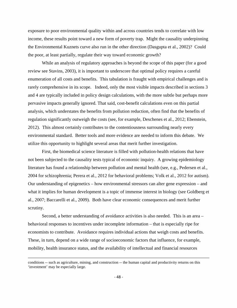
‐ 48 ‐
exposure to poor environmental quality within and across countries tends to correlate with low
income, these results point toward a new form of poverty trap. Might the causality underpinning
the Environmental Kuznets curve also run in the other direction (Dasgupta et al., 2002)? Could
the poor, at least partially, regulate their way toward economic growth?
While an analysis of regulatory approaches is beyond the scope of this paper (for a good
review see Stavins, 2003), it is important to underscore that optimal policy requires a careful
enumeration of all costs and benefits. This tabulation is fraught with empirical challenges and is
rarely comprehensive in its scope. Indeed, only the most visible impacts described in sections 3
and 4 are typically included in policy design calculations, with the more subtle but perhaps more
pervasive impacts generally ignored. That said, cost-benefit calculations even on this partial
analysis, which understates the benefits from pollution reduction, often find that the benefits of
regulation significantly outweigh the costs (see, for example, Deschenes et al., 2012; Ebenstein,
2012). This almost certainly contributes to the contentiousness surrounding nearly every
environmental standard. Better tools and more evidence are needed to inform this debate. We
utilize this opportunity to highlight several areas that merit further investigation.
First, the biomedical science literature is filled with pollution-health relations that have
not been subjected to the causality tests typical of economic inquiry. A growing epidemiology
literature has found a relationship between pollution and mental health (see, e.g., Pedersen et al.,
2004 for schizophrenia; Perera et al., 2012 for behavioral problems; Volk et al., 2012 for autism).
Our understanding of epigenetics – how environmental stressors can alter gene expression – and
what it implies for human development is a topic of immense interest in biology (see Goldberg et
al., 2007; Baccarelli et al., 2009). Both have clear economic consequences and merit further
scrutiny.
Second, a better understanding of avoidance activities is also needed. This is an area –
behavioral responses to incentives under incomplete information – that is especially ripe for
economists to contribute. Avoidance requires individual actions that weigh costs and benefits.
These, in turn, depend on a wide range of socioeconomic factors that influence, for example,
mobility, health insurance status, and the availability of intellectual and financial resources
conditions -- such as agriculture, mining, and construction -- the human capital and productivity returns on this ‘investment’ may be especially large.
‐ 49 ‐
required to avert. For those pollutants with subtle impacts, models of learning and inattention
may be particularly important. The current stalemate on actions to avert climate change suggests
that avoidance and adaptation are likely to play an increasingly large role in global welfare going
forward.
Lastly, the evidence on human capital and especially labor market effects from pollution
exposure are just beginning to emerge. Despite its beginning stages, the limited evidence thus far
suggests negative impacts on cognitive ability, school performance, and job performance. Much
more should be done to replicate these results in other contexts and to unpack the mechanisms
driving them, which in turn will help to generalize them beyond the narrow settings that have
thus far been necessary to pin down empirical identification.
The collection of environmental, health, and human capital data is being rapidly
transformed. The past decade has witnessed a proliferation of cheaper and more sophisticated
environmental sensors as well as significant improvements in the science that allow us to
transform satellite data into meaningful measures of environmental conditions on the ground.
The proliferation of electronic surveillance and data capture in schools and the workplace,
combined with increased digitization and linkage of historical data, has significantly increased
access to not only better human capital and productivity data but also to data that spans a lifetime
of exposures, encounters, and outcomes.60 These advances promise to improve the resolution and
scope of our analytic purview. Ironically, these improvements are occurring at the same time
that access to finely geocoded health data, which have been the mainstay of research in this area,
are being threatened by proposed NIH revisions regarding data confidentiality. Nonetheless, we
remain optimistic about to the prospects for deepening our understanding of the role played by
the environment as a largely ignored factor production in the coming decades.
60 Examples of longitudinal data sets that cover multiple life stages include the National Children's Study (underway), birth data linked with health and schooling outcomes in Sweden and Chile (see, for example, Almond et al., 2009, Nilsson 2009, and Bharadwaj et al., 2012), and linked National Health Service data from England.
‐ 50 ‐
References Agarwal, Nikhil, Chanont Banterghansa, Linda Bui. "Toxic Exposure in America: Measuring Fetal and Infant Health Outcomes from 14 years of TRI Reporting." Journal of Health Economics 29. 4 (2010): 557-574. Almond, Douglas, Kenneth Chay and David Lee (2005). "The Costs of Low Birth Weight." The Quarterly Journal of Ecnomics 120(3): 1031-1083. Almond, Douglas and Janet Currie (2011). “Killing Me Softly: The Fetal Origins Hypothesis,” the Journal of Economic Perspectives, 25(3), 153-72. Almond, Douglas, Lena Edlund and Mårten Palme (2009). "Chernobyl's Subclinical Legacy: Prenatal Exposure to Radioactive Fallout and School Outcomes in Sweden." The Quarterly Journal of Economics 124(4): 1729-1772. Auffhammer, Maximilian, and Ryan Kellogg. "Clearing the Air? The Effects of Gasoline Content Regulation on Air Quality." The American Economic Review 101.6 (2011): 2687-2722. Baccarelli A, Wright RO, Bollati V, Tarantini L, Litonjua AA, Suh HH, Zanobetti A, Sparrow D, Vokonas PS, Schwartz J. “Rapid DNA methylation changes after exposure to traffic particles.” Am J Respir Crit Care Med. 2009 Apr 1;179(7):572-8. Banzhaf, H. Spencer and Randall P. Walsh, 2008. "Do People Vote with Their Feet? An Empirical Test of Tiebout," American Economic Review, 98(3): 843-63. Bayer, Patrick, Bryan Ellickson, Paul Ellickson. (May, 2010). Dynamic Asset Pricing in a System of Local Housing Markets. American Economics Association Papers and Proceedings Bartik, T. J. Evaluating the benefits of non-marginal reductions in pollution using information on defensive expenditures, J. Enriron. Econom. Management 15, 111-127 (1988). Behrman, Jere R., Mark R. Rosenzweig, and Paul Taubman (1994). "Endowments and the Allocation of Schooling in the Family and in the Marriage Market: The Twins Experiment." Journal of Political Economy, 102: 1131-1174. Bell M, Samet JM, Dominici F (2004). "Time-Series Studies of Particulate Matter," Annual Review of Public Health, 25:247-280. Bharadwaj, Prashant, Katrine Loken, and Christopher Neilson. (2012) “Early Childhood Health Interventions and Academic Achievement.” American Economic Review, forthcoming.
‐ 51 ‐
Black, Sandra, Paul Devereux and Kjell Salvanes. “From the Cradle to the Labor Market? The Effect of Birth Weight on Adult Outcomes,” Quarterly Journal of Economics 122 (2007) 409-439. Block, Michelle and Lilian Calderón-Garcidueñas (2009). " Air Pollution: Mechanisms of Neuroinflammation & CNS Disease." Trends Neurosci. 2009 September ; 32(9): 506–516. Braden, J. B. and C. D. Kolstad (1991). Measuring the demand for environmental quality. New York: North-Holland. Brimblecombe, Peter (1999). The Big Smoke: A History of Air Pollution in London Since Medieval Times. Cambridge University Press: London, England Buck Louis GM, Dmochowski J, Lynch CD, Kostyniak PJ, McGuinness BM, Vena JE. (2009). Polychlorinated biphenyl concentrations, lifestyle and time-to-pregnancy. Hum Reprod 24:451-458. Card, David, Carlos Dobkin, and Nicole Maestas (2009). "Does Medicare Save Lives?" Quarterly Journal of Economics, Vol. 124, No. 2, pp. 597–636. Carson, Richard, Phoebe Koundouri, and Céline Nauges (2010). “Arsenic Mitigation in Bangladesh: A Household Labor Market Approach.” American Journal of Agricultural Economics, 92. Chay, Kenneth and Michael Greenstone (2003a). “The Impact of Air Pollution on Infant Mortality: Evidence from Geographic Variation in Pollution Shocks Induced by a Recession.” Quarterly Journal of Economics, 118(3): 1121-1167. Chay, Kenneth and Michael Greenstone (2003b). " Air Quality, Infant Mortality, and the Clean Air Act of 1970." NBER Working Paper 10053. Chay, Kenneth and Michael Greenstone (2005). “Does Air Quality Matter? Evidence from the Housing Market.” Journal of Political Economy, 113: 376–424 Chay, Kenneth, Carlos Dobkin and Michael Greenstone (2003). "The Clean Air Act of 1970 and Adult Mortality." Journal of Risk and Uncertainty, 27(3). Chen, Yuyu, Ginger Zhe Jin, Naresh Kumar, and Guang Shi (2013). "Gaming in Air Pollution Data? Lessons from China." NBER Working Paper 18729. Clay, Karen, Werner Troesken, and Michael Haines (2010). "Lead, Mortality, and Productivity." NBER Working Paper 16480. Clougherty JE, Kheirbek I, Johnson S, Pezeshki G, Jacobson JB, Kass D, et al. The New York City
‐ 52 ‐
Community Air Survey: results from winter monitoring 2008–2009 [Internet]. New York (NY): NYC Health, PlaNYC; 2009 [cited 2011 Nov 14]. Available from: http://www.nyc.gov/html/doh/downloads/pdf/eode/comm-air-survey-reportwinter08-09.pdf Courant, P. N. and R. Porter, Averting expenditure and the cost of pollution, J. Enriron. Econom. Management 8,321-329 (1981). Crocker, Thomas and Robert Horst (1981). "Hours of Work, Labor Productivity, and Environmental-Conditions : A Case Study." Review of Economics and Statistics 63(3): 361-368. Cropper, M. L., & Freeman, A. M., III. (1991). Environmental health effects. In J. B. Braden, & C. D. Kolstad (Eds.), Measuring the demand for environmental quality. New York: North-Holland. Cropper, Maureen and Wallace Oates, “Environmental Economics: A Survey,” Journal of Economic Literature 30(2), 1992. Cunha, Flavio and James Heckman (2007). "The Technology of Skill Formation," American Economic Review, American Economic Association, 97(2):31-47. Cunningham FG, Leveno KJ, Bloom SL, et al. Fetal growth and development. In: Cunnigham FG, Leveno KL, Bloom SL, Hauth, JC, Rouse DJ, Spong CY, eds. Williams Obstetrics. 23rd ed. New York, NY: McGraw-Hill; 2010:chap 4 Currie, Janet, and Rosemary Hyson (1999). "Is the Impact of Health Shocks Cushioned by Socioeconomic Status? The Case of Low Birthweight." American Economic Review, 89(2): 245-250. Currie, Janet and Brigitte Madrian (1999). "Health, Health Insurance and the Labor Market," The Handbook of Labor Economics, volume 3c, David Card and Orley Ashenfelter (eds.), Amsterdam: North Holland, 1999, 3309-3407. Currie, Janet and Johannes Schmieder (2009). "Fetal Exposure to Toxic Releases and Infant Health,” American Economic Association Papers and Proceedings, 99(2), 177-83. Currie, Janet and Matthew Neidell (2005). “Air Pollution and Infant Health: What Can We Learn from California's Recent Experience?” Quarterly Journal of Economics, 120(3): 1003-1030. Currie, Janet and Mark Stabile (2006). "Child mental health and human capital accumulation: The case of ADHD," Journal of Health Economics, 25(6): 1094-1118. Currie, Janet, Eric Hanushek, E. Megan Kahn, Matthew Neidell and Steven Rivkin (2009a). "Does Pollution Increase School Absences?" Review of Economics and Statistics 91(4), 2009. Currie, Janet, Matthew Neidell and Johannes Schmieder (2009b). "Air Pollution and Infant Health: Lessons from New Jersey." Journal of Health Economics, 28(3).
‐ 53 ‐
Currie, Janet. 2011. “Inequality at Birth: Some Causes and Consequences,” American Economic Review Papers and Proceedings. Currie, Janet and Duncan Thomas (2001). "Early test scores, school quality, and SES: longrun effects on wage and employment outcomes." In: Polachek S, editor. Worker wellbeing in a changing labor market. Vol. 20, Research in labor economics. Bingley (UK): Emerald Group Publishing Ltd. Currie, Janet and Reed Walker (2011). "Traffic Congestion and Infant Health: Evidence from E-ZPass." American Economic Journal: Applied Economics, 3(1): 65-90. Currie, Janet, Joshua Graff Zivin, Katherine Meckel, Matthew Neidell, and Wolfram Schlenker, “Something in the Water: Contaminated Drinking Water and Infant Health,” NBER Working Paper 18876, 2013.
Currie, Janet, Lucas Davis, Michael Greenstone, and Reed Walker, “Do Housing Prices Reflect Environmental Health Risks? Evidence from More than 1600 Toxic Plant Openings and Closings,” NBER Working Paper #18700, 2013.
Cutler, David, Angus Deaton, and Adriana Lleras-Muney (2006). "The Determinants of Mortality." Journal of Economic Perspectives, 20(3). Cutler, David "The Lifetime Costs and Benefits of Medical Technology," Journal of Health Economics, 26(6), 2007, 1081-1100. Dasgupta, S., Laplante, B., Wang, H., & Wheeler, D. (2002). Confronting the environmental Kuznets curve. Journal of Economic Perspectives, 16, 147–168. Davidson, C.I., W. Tang, S. Finger, V. Etyemezian, M. F. Striegel, and S.I. Sherwood, “Soiling Patterns on a Tall Limestone Building: Changes Over Sixty Years,” Environmental Science and Technology, Vol. 34, pp. 560-565, 2000. de Graaf-Peters VB, Hadders-Algra M. “Ontogeny of the human central nervous system: what is happening when?” Early Hum Development 2006 Apr;82(4):257-66. Deleire, Thomas, Shakeeb Khan and Christopher Timmins (2011). "Roy Model Sorting and Non-Random Selection in the Valuation of a Statistical Life," International Economic Review, forthcoming. Deschenes, Olivier (2012). “Temperature, Human Health, and Adaptation: A Review of the Empirical Literatures.” NBER Working Paper 18345. Deschenes, Olivier and Michael Greenstone (2011). “Climate Change, Mortality, and
‐ 54 ‐
Adaptation: Evidence from Annual Fluctuations in Weather in the US.” American Economic Journal: Applied Economics,3(4): 152-185. Deschenes, Olivier, Michael Greenstone and Joseph Shapiro (2012). “Defensive Investments and the Demand for Air Quality: Evidence from the NOx Budget Program and Ozone Reductions." NBER Working Paper 18267. Dimeo MJ, Glenn MG, Holtzman MJ, Sheller JR, Nadel JA, Boushey HA. Threshold concentration of ozone causing an increase in bronchial reactivity in humans and adaptation with repeated exposures. Am Rev Respir Dis. 1981 Sep;124(3):245-8.
Dominici F, Samet JM, Zeger SL (2000). "Combining Evidence on Air pollution and Daily Mortality from the Twenty Largest US Cities: A Hierarchical Modeling Strategy," Royal Statistical Society, Series A, with discussion, 163(3):263-302, read at the Royal Statistical Society, London, January 10, 2000. Dominici F, Daniels M, Zeger SL, Samet JM (2002). "Air Pollution and Mortality: Estimating Regional and National Dose-Response Relationships," Journal of the American Statistical Association, 97(457):100-111. Dominici F, Wang C, Crainiceanu CM, Parmigiani G. (2008) Model Selection and Health Effect Estimation in Environmental Epidemiology, Epidemiology, 19, 558-560. Ebenstein, Avraham (2012). "The Consequences of Industrialization: Evidence from Water Pollution and Digestive Cancers in China," Review of Economics and Statistics, 94(1):186-201 Firket J. 1936. Fog along the Meuse Valley. Trans. Faraday Soc. 32:1192–97. Finkelstein, Amy, Sarah Taubman, Bill Wright, Mira Bernstein, Jonathan Gruber, Joseph P. Newhouse, Heidi Allen, and Katherine Baicker (2011). "The Oregon health insurance experiment: evidence from the first year." National Bureau of Economic Research Working Paper 17190. Folinsbee, L. J., McDonnell, W. F., & Horstman, D. H. (1988). Pulmonary function and symptom responses after 6.6-hour exposure to 0.12 ppm ozone with moderate exercise. Japca, 38(1), 28-35. Goldberg, Aaron D., C. David Allis, and Emily Bernstein. "Epigenetics: a landscape takes shape." Cell 128.4 (2007): 635. Graff Zivin, Joshua, Matthew Neidell and Wolfram Schlenker (2011). "Water Quality Violations and Avoidance Behavior: Evidence from Bottled Water Consumption." American Economic Review: Papers and Proceedings, 101(3).
‐ 55 ‐
Graff Zivin, Joshua and Matthew Neidell (2009). “Days of Haze: Environmental Information Disclosure and Intertemporal Avoidance Behavior." Journal of Environmental Economics and Management, 58(2). Graff Zivin, Joshua and Matthew Neidell (2012). “The impact of pollution on worker productivity.” American Economic Review, forthcoming. Greenburg L, Jacobs MB, Drolette BM, Field F, Braverman MM. 1962. "Report of an air pollution incident in New York City, November 1953." Public Health Rep. 77:7–16 Grossman, Michael (1972). "On the Concept of Health Capital and the Demand for Health." Journal of Political Economy 80(2). Grossman, Michael and Robert Kaestner (1997). “The Effects of Education on Health,” in The Social Benefits of Education, Jere Behrman and Nancy Stacy (editors) (Ann Arbor: University of Michigan Press). Hanna, Rema and Paulina Oliva (2011). “The Effect of Pollution on Labor Supply: Evidence from a Natural Experiment in Mexico City.” NBER Working Paper 17302. Harrington, W. and P. R. Portney, Valuing the benefits of health and safety regulations, J . Urban Econom. 22, 101-112 (1987). Hazucha, Milan, Lawrence Folinsbee, and Philip Bromberg. 2003. “Distribution and Reproducibility of Spirometric Response to Ozone by Gender and Age.” Journal of Applied Physiology, 95: 1917-1925.
Huff, James, and Joseph Haseman. "Long-term chemical carcinogenesis experiments for identifying potential human cancer hazards: collective database of the National Cancer Institute and National Toxicology Program (1976-1991)." Environmental health perspectives 96 (1991): 23. Institute of Medicine, 2002. Unequal Treatment: Confronting Racial and Ethnic Disparities in Health Care. National Academy Press, Washington, DC. International Labour Organization (2011). Global Employment Trends 2011: The Challenge of a Jobs Recovery. Geneva, Switzerland: International Labour Organization. Janes H, Dominici F, Zeger SL (2007). "Trends in Particulate Matter and Mortality in 113 U.S. Counties, 2000-2002: Evidence on the Long Term Effects of Air Pollution." Epidemiology, 18: 416-423. Jayachandran, Seema (2009). " Air Quality and Early-Life Mortality: Evidence from Indonesia's Wildfires." Journal of Human Resources, 44 (4), pp. 916-954.
‐ 56 ‐
Jerrett M, Arain A, Kanaroglou P, Beckerman B, Potoglou D, Sahsuvaroglu T, Morrison J, Giovis C. (2005). "A review and evaluation of intraurban air pollution exposure models." J Expos Anal Environ Epidemiol. 15:185–204. Jerrett, Michael, Richard T. Burnett, C. Arden Pope, III, Kazuhiko Ito, George Thurston, Daniel Krewski, Yuanli Shi, Eugenia Calle, and Michael Thun (2009). " Long-Term Ozone Exposure and Mortality." N Engl J Med 360:1085-109 Jones, N. C., Thornton, C. A., Mark, D., & Harrison, R. M. (2000). Indoor/outdoor relationships of particulate matter in domestic homes with roadside, urban and rural locations. Atmospheric Environment, 34(16), 2603-2612. Joyce, T., Grossman, M. and F. Goldman (1988). "An Assessment of the Benefits of Air Pollution Control: The Case of Infant Health." Journal of Urban Economics 25: 32-51. Kampa, Marilena, and Elias Castanas. "Human health effects of air pollution." Environmental Pollution 151.2 (2008): 362-367. Kaufman JD, Adar SD, Allen RW, Barr RG, Budoff MJ, Burke GL, Casillas AM, Cohen MA, Curl CL, Daviglus ML, Diez Roux AV, Jacobs DR Jr, Kronmal RA, Larson TV, Liu SL, Lumley T, Navas-Acien A, O'Leary DH, Rotter JI, Sampson PD, Sheppard L, Siscovick DS, Stein JH, Szpiro AA, Tracy RP. “Prospective Study of Particulate Air Pollution Exposures, Subclinical Atherosclerosis, and Clinical Cardiovascular Disease: The Multi-Ethnic Study of Atherosclerosis and Air Pollution (MESA Air).” American Journal of Epidemiology 2012 Nov 1;176(9):825-37. Knittel, Christopher, Douglas Miller and Nick Sanders (2011). “Caution Drivers! Children Present. Traffic, Pollution, and Infant Health,” NBER Working Paper 17222. Lavy, Victor, Avraham Ebenstein, Sefi Roth (2012). "Ambient Air Pollution, Cognitive Performance, and Long Term Consequences for Human Capital Formation." Mimeo, Hebrew University of Jerusalem. Le Tertre A, Medina S, Samoli E, Forsberg B, Michelozzi P, Boumghar A, Vonk JM, Bellini A, Atkinson R, Ayres JG, Sunyer J, Schwartz J, Katsouyanni K. “Short-term effects of particulate air pollution on cardiovascular diseases in eight European cities.” Journal of Epidemiology and Community Health. 2002 Oct;56(10):773-9. Lefohn AS, Hazucha MJ, Shadwick D, Adams WC. “An alternative form and level of the human health ozone standard.” Inhalation Toxicology 2010 Oct;22(12):999-1011. Lichtenberg, Frank “The Impact of New Drugs on U.S. Longevity and Medical Expenditure, 1990-2003,”American Economic Review 97 (2), May 2007, 438-443.
‐ 57 ‐
Lleras-Muney, Adriana (2010). "The Needs of the Army: Using Compulsory Relocation in the Military to Estimate the Effect of Air Pollutants on Children's Health." Journal of Human Resources. 45(3):549-90. Logan, W. P. D., and M. D. Glasg, “Mortality in London Fog Incident, 1952,” Lancet, I (1953), 336–338. Madajewicz, M., A. Pfaff, J. Graziano, A. van Geen, I. Hussein, H. Momotaj, R. Sylvi & H. Ahsan (2007). "Can Information Alone Both Improve Awareness and Change Behavior? Arsenic contamination of groundwater in Bangladesh." Journal of Development Economics 84(2): 731-754. Magat, Wesley and W. Kip Viscusi. Informational Approaches to Regulation, Cambridge, MA: The MIT Press, 1992. Manning, Willard G., Joseph P. Newhouse, Naihua Duan, Emmett B. Keeler, and Arleen Leibowitz. "Health insurance and the demand for medical care: evidence from a randomized experiment." The American Economic Review (1987): 251-277. Martin, Randall V. "Satellite remote sensing of surface air quality." Atmospheric Environment 42.34 (2008): 7823-7843.
McCllelan, Mark (1998). “Health Events, Health Insurance, and Labor Supply: Evidence from the Health and Retirement Survey,” in David A. Wise, ed., Frontiers in the Economics of Aging, Chicago: University of Chicago Press.
Miller KA, Siscovick DS, Sheppard L, Shepherd K, Sullivan JH, Anderson GL, Kaufman JD. (2007). Long-term exposure to air pollution and incidence of cardiovascular events in women. N Engl J Med 356:447-458 Moretti, Enrico and Matthew Neidell (2011). " Pollution, Health, and Avoidance Behavior: Evidence from the Ports of Los Angeles." Journal of Human Resources 46(1), 2011 Moulton, Brent (1986). "Random group effects and the precision of regression estimates," Journal of Econometrics, 32(3): 385-397. Neidell, Matthew (2009). “Information, Avoidance Behavior, and Health: The Effect of Ozone on Asthma Hospitalizations.” Journal of Human Resources, 44(2). Nelson, Richard R., and Edmund S. Phelps. "Investment in humans, technological diffusion, and economic growth." The American Economic Review (1966): 69-75. Nilsson, J. Peter (2009). " The Long run effects of Early Childhood Lead Exposure: Evidence from the Phase-out of Leaded Gasoline." Mimeo, Institute for International Economic Studies.
‐ 58 ‐
Oreopoulos P, Stabile M, Walld R, Roos LL (2008). "Short-, medium-, and long-term consequences of poor infant health: an analysis using siblings and twins." Journal of Human Resources, 43(1):88–138.
Pauly, Mark, Sean Nicholson, Daniel Polsky, Marc Berger and Claire Sharda (2008). “Valuing Reductions in on-the-Job Illness: ‘Presenteeism’ from Managerial and Economic Perspectives.” Health Economics, 17: 469–485.
Pedersen CB, Raaschou-Nielsen O, Hertel O, Mortensen PB. “Air pollution from traffic and schizophrenia risk.” Schizophrenia Research 2004 Jan 1;66(1):83-5. Peng R, Dominici F, Louis T (2006). "Model Choice in Multi-Site Time Series Studies of Air Pollution and Mortality," Journal of the Royal Statistical Society, Series A 169, Part 2:179-203. Perera FP, Tang D, Wang S, Vishnevetsky J, Zhang B, Diaz D, Camann D, Rauh V (2012). "Prenatal polycyclic aromatic hydrocarbon (PAH) exposure and child behavior at age 6-7" Environ Health Perspect 120(6):921-6. Pope, C. Arden (1989). "Respiratory Disease Associated with Community Air Pollution and a Steel Mill." American Journal of Public Health. 79(5):623-28. Pope CA III, Burnett RT, Thun MJ, Calle EE, Krewski D, Ito K, Thurston GD. (2002). "Lung cancer, cardiopulmonary mortality, and long-term exposure to fine particulate air pollution. " JAMA 287:1132-1141. Pope CA 3rd, Hansen JC, Kuprov R, Sanders MD, Anderson MN, Eatough DJ. “Vascular function and short-term exposure to fine particulate air pollution.” Journal of the Air and Waste Management Association 2011 Aug;61(8):858-63. Pottenger LH, Schisler MR, Zhang F, Bartels MJ, Fontaine DD, McFadden LG, Bhaskar Gollapudi B. “Dose-response and operational thresholds/NOAELs for in vitro mutagenic effects from DNA-reactive mutagens, MMS and MNU.” Mutation Research 2009 Aug;678(2):138-47. Ransom, Michael and C. Arden Pope (1992). "Elementary School Absences and PM10 Pollution in Utah Valley." Environmental Research. 58(2):204-19. Ransom, Michael C. Arden Pope (1995). "Estimating external health costs of a steel mill." Contemp Econ Policy. 13: 86–97. Rawski, Thomas (2009). "Urban Air Quality in China: Historical and Comparative Perspective." In Resurgent China: Issues for the Future, edited by Nazrul Islam. Reyes, Jessica (2007). “Environmental Policy as Social Policy? The Impact of Childhood Lead Exposure on Crime,” B.E. Journal of Economic Analysis and Policy, 7:1 (Contributions).
‐ 59 ‐
Roback, Jennifer (1982) ”Wages, Rents, and the Quality of Life.” Journal of Political Economy, 90, pp. 1257-1278. Romer, Paul. Increasing returns and long-run growth The Journal of Political Economy, 94 (1986) Rojas-Martinez R, Perez-Padilla R, Olaiz-Fernandez G, Mendoza-Alvarado L, Moreno-Macias H, Fortoul T, McDonnell W, Loomis D, Romieu I. (2007). Lung function growth in children with long-term exposure to air pollutants in Mexico City. Am J Respir Crit Care Med 176:377-384 Royer, Heather (2009). "Separated at girth: US twin estimates of the effects of birth weight." American Economic Journal: Applied Economics, 1:49–85.
Sacks, Jason D; Ito, Kazuhiko; Wilson, William E; Neas, Lucas M (2012). "Impact of covariate models on the assessment of the air pollution-mortality association in a single- and multipollutant context." American journal of epidemiology, 176: 622:622-634. Sanders, Nick (2012). “What Doesn’t Kill You Makes Your Weaker: Prenatal Pollution Exposure and Educational Outcomes,” Journal of Human Resources, 47(3): 826-850. Salam, M. T., Millstein, J., Li, Y. F., Lurmann, F. W., Margolis, H. G., & Gilliland, F. D. (2005). Birth outcomes and prenatal exposure to ozone, carbon monoxide, and particulate matter: results from the Children’s Health Study. Environmental health perspectives, 113(11), 1638. Sanders, Nick and Charles Stoecker (2011). “Where Have All the Young Men Gone? Using Sex Ratios to Measure Fetal Death Rates.” NBER Working Paper 17434. Schlenker, Wolfram and Reed Walker (2011). "Airports, Air Pollution, and Contemporaneous Health." NBER Working Paper #17684. Schultz, T. Investment in human capital. The American Economic Review, 51 (1961), pp. 1–17 Seigneur, Christian, Krish Vijayaraghavan, Kristen Lohman, Prakash Karamchandani, and Courtney Scott, “Global Source Attribution for Mercury Deposition in the United States.” Environ. Sci. Technol., 2004, 38 (2): 555–569.
Sen, Amartya. (1992): “Missing Women,” British Medical Journal, 304, 586–87. Schwartz, Joel (2004). "Air pollution and children's health." Pediatrics. 113(4 Suppl):1037-43. Shimshack, Jay Michael Ward, and Tim Beatty. 2007. Mercury Advisories: Information, Education, and Fish Consumption. Journal of Environmental Economics and Management 53(2): 158-79.
‐ 60 ‐
Singh S, Loke YK, Enright PL, Furberg CD (2011). "Mortality associated with tiotropium mist inhaler in patients with chronic obstructive pulmonary disease: systematic review and meta-analysis of randomised controlled trials." British Medical Journal. 14;342:d3215. Skerfving S, Bergdahl IA. (2007) Chapter 31. “Lead”, In: Nordberg GF, Fowler BA, Nordberg M, Friberg LT. Handbook on the Toxicology of Metals, Academic Press, Elsevier, p.599-643. ISBN 978-0-369413-3. Smith, James P (2003). “Consequences and Predictors of New Health Events,” in David A. Wise, ed., Analyses in the Economics of Aging, Chicago: University of Chicago Press. Smith KR, Peel JL. “Mind the gap.” Environmental Health Perspectives 2010 Dec;118(12):1643-5. Stavins, Robert 2003. Experience with Market-Based Environmental Policy Instruments. In: K. Maler and J.R. Vincent Eds., Handbook of environmental economics. Volume 1. Environmental degradation and institutional responses. Handbooks in Economics, vol. 20. Amsterdam; Boston and London: Elsevier Science, North-Holland, pp. 355-435. Stoeger T, Reinhard C, Takenaka S, Schroeppel A, Karg E, Ritter B, Heyder J, Schulz H. “Instillation of six different ultrafine carbon particles indicates a surface area threshold dose for acute lung inflammation in mice.” Environmental Health Perspectives 2006 Mar;114(3):328-33. Strauss, John and Duncan Thomas. 1998. “Health, Nutrition, and Economic Development.” Journal of Economic Literature. 36: 766-817. Tiebout, Charles. (1956), "A Pure Theory of Local Expenditures", Journal of Political Economy 64 (5): 416–424. Tonne, Cathryn, Robin Whyatt, David Camann, Frederica Perera, and Patrick Kinney (2004). " Predictors of personal polycyclic aromatic hydrocarbon exposures among pregnant minority women in New York City." Environ Health Perspect. 112(6): 754–759. Townsend, JG (1950). "Investigation of the smog incident in Donora, Pa., and vicinity." Am J Public Health Nations Health. 40(2):183-9. Trivers, Robert L. and Dan E. Willard (1973). “Natural Selection of Parental Ability to Vary the Sex Ratio of Offspring.” Science 179 (4068):90. Troesken, Werner. "Lead Water Pipes and Infant Mortality in Turn-of-the-Century Massachusetts" Journal of Human Resources, vol. 43, no. 3 (Dec., 2008), pp. 553-75. Vahlsing, Candace and Kirk Smith (2011). "Global review of national ambient air quality standards for PM10 and SO2 (24 h)." Air Quality, Atmosphere and Health, 1-7.

‐ 61 ‐
Volk, Heather E., Fred Lurmann, Bryan Penfold, Irva Hertz-Picciotto, Rob McConnell (2012). " Traffic-Related Air Pollution, Particulate Matter, and Autism." Archives of General Psychiatry, Online First, 1-7. Zweig, Jacqueline, John Ham and Edward Avol (2009). "Air pollution and Academic Performance: Evidence from California Schools." Mimeo, University of Southern California.
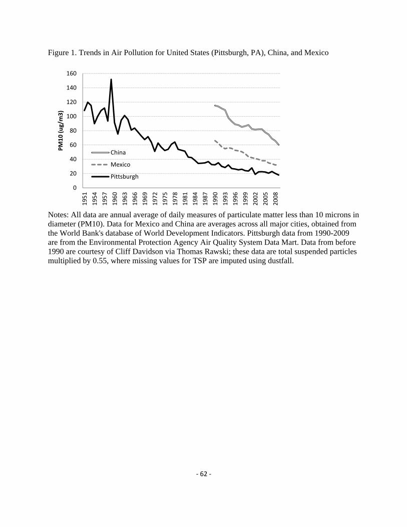
‐ 62 ‐
Figure 1. Trends in Air Pollution for United States (Pittsburgh, PA), China, and Mexico
Notes: All data are annual average of daily measures of particulate matter less than 10 microns in diameter (PM10). Data for Mexico and China are averages across all major cities, obtained from the World Bank's database of World Development Indicators. Pittsburgh data from 1990-2009 are from the Environmental Protection Agency Air Quality System Data Mart. Data from before 1990 are courtesy of Cliff Davidson via Thomas Rawski; these data are total suspended particles multiplied by 0.55, where missing values for TSP are imputed using dustfall.
0
20
40
60
80
100
120
140
160
1951
1954
1957
1960
1963
1966
1969
1972
1975
1978
1981
1984
1987
1990
1993
1996
1999
2002
2005
2008
PM10 (ug/m3)
China
Mexico
Pittsburgh
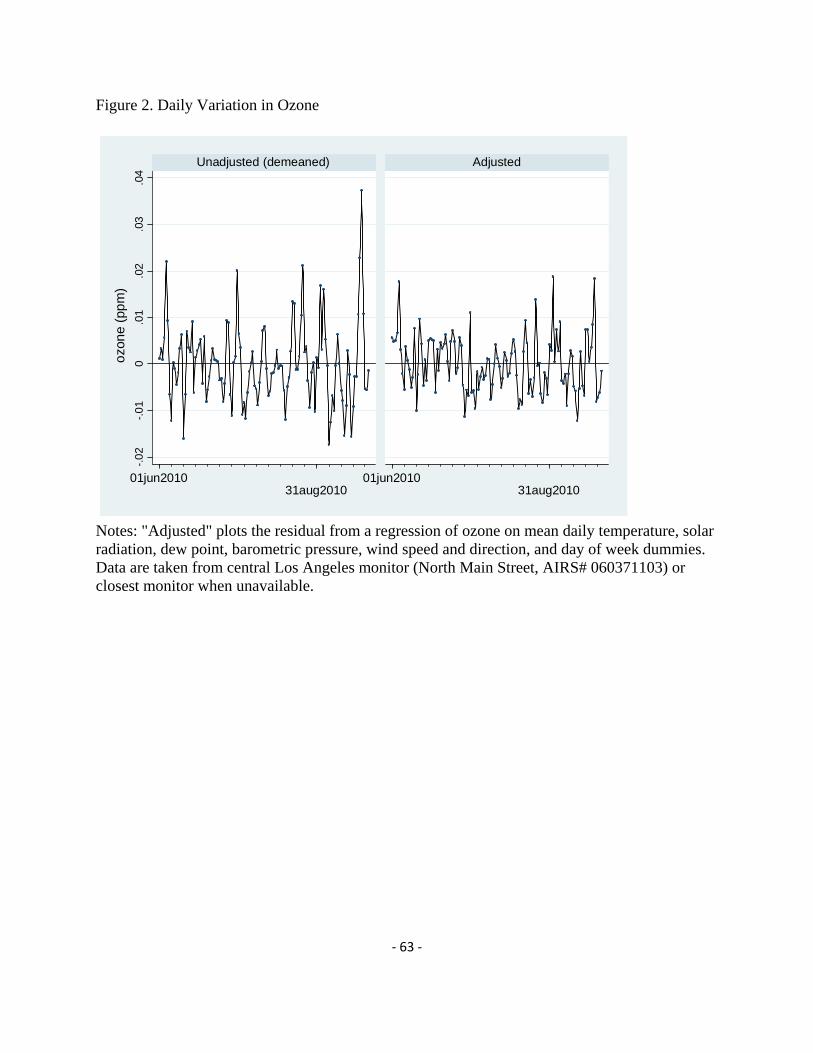
‐ 63 ‐
Figure 2. Daily Variation in Ozone
Notes: "Adjusted" plots the residual from a regression of ozone on mean daily temperature, solar radiation, dew point, barometric pressure, wind speed and direction, and day of week dummies. Data are taken from central Los Angeles monitor (North Main Street, AIRS# 060371103) or closest monitor when unavailable.
-.0
2-.
01
0.0
1.0
2.0
3.0
4
01jun201031aug2010
01jun201031aug2010
Unadjusted (demeaned) Adjusted
ozo
ne
(pp
m)
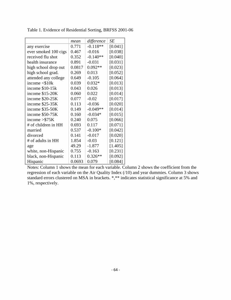
‐ 64 ‐
Table 1. Evidence of Residential Sorting, BRFSS 2001-06 mean difference SE any exercise 0.771 -0.118** [0.041]ever smoked 100 cigs 0.467 -0.016 [0.038]received flu shot 0.352 -0.140** [0.040]health insurance 0.891 -0.031 [0.031]high school drop out 0.0817 0.092** [0.023]high school grad. 0.269 0.013 [0.052]attended any college 0.649 -0.105 [0.064]income <$10k 0.039 0.032* [0.013]income $10-15k 0.043 0.026 [0.013]income $15-20K 0.060 0.022 [0.014]income $20-25K 0.077 -0.02 [0.017]income $25-35K 0.113 -0.036 [0.020]income $35-50K 0.149 -0.049** [0.014]income $50-75K 0.160 -0.034* [0.015]income >$75K 0.240 0.075 [0.066]# of children in HH 0.693 0.117 [0.071]married 0.537 -0.100* [0.042]divorced 0.141 -0.017 [0.020]# of adults in HH 1.854 -0.03 [0.121]age 49.29 -1.877 [1.405]white, non-Hispanic 0.755 -0.163 [0.231]black, non-Hispanic 0.113 0.326** [0.092]Hispanic 0.0693 0.079 [0.084]Notes: Column 1 shows the mean for each variable. Column 2 shows the coefficient from the regression of each variable on the Air Quality Index (/10) and year dummies. Column 3 shows standard errors clustered on MSA in brackets. *,** indicates statistical significance at 5% and 1%, respectively.
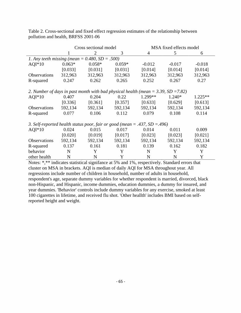
‐ 65 ‐
Table 2. Cross-sectional and fixed effect regression estimates of the relationship between pollution and health, BRFSS 2001-06 Cross sectional model MSA fixed effects model 1 2 3 4 5 6 1. Any teeth missing (mean = 0.480, SD = .500) AQI*10 0.063* 0.058* 0.059* -0.012 -0.017 -0.018 [0.033] [0.031] [0.031] [0.014] [0.014] [0.014] Observations 312,963 312,963 312,963 312,963 312,963 312,963 R-squared 0.247 0.262 0.265 0.252 0.267 0.27 2. Number of days in past month with bad physical health (mean = 3.39, SD =7.82) AQI*10 0.407 0.204 0.22 1.299** 1.240* 1.225** [0.336] [0.361] [0.357] [0.633] [0.629] [0.613] Observations 592,134 592,134 592,134 592,134 592,134 592,134 R-squared 0.077 0.106 0.112 0.079 0.108 0.114 3. Self-reported health status poor, fair or good (mean = .437, SD =.496) AQI*10 0.024 0.015 0.017 0.014 0.011 0.009 [0.020] [0.019] [0.017] [0.023] [0.023] [0.021] Observations 592,134 592,134 592,134 592,134 592,134 592,134 R-squared 0.137 0.161 0.181 0.139 0.162 0.182 behavior N Y Y N Y Y other health N N Y N N Y Notes: *,** indicates statistical signifance at 5% and 1%, respectively. Standard errors that cluster on MSA in brackets. AQI is median of daily AQI for MSA throughout year. All regressions include number of children in household, number of adults in household, respondent's age, separate dummy variables for whether respondent is married, divorced, black non-Hispanic, and Hispanic, income dummies, education dummies, a dummy for insured, and year dummies. 'Behavior' controls include dummy variables for any exercise, smoked at least 100 cigarettes in lifetime, and received flu shot. 'Other heallth' includes BMI based on self-reported height and weight.


![Outline Human capital theory by C. Echevarriahomepage.usask.ca/~ece220/econ221/4-HC [Compatibility Mode].pdf · Human capital theory by C. Echevarria ... Human capital Human capital](https://static.fdocuments.in/doc/165x107/5ae0d5467f8b9a6e5c8df29c/outline-human-capital-theory-by-c-ece220econ2214-hc-compatibility-modepdfhuman.jpg)


