ENTRY TRAJECTORY AND ATMOSPHERE RECONSTRUCTION METHODOLOGIES FOR THE MARS EXPLORATION ROVER MISSION

Prasun N. Desai('), Robert C. Blanchard"), Richard W. Powell")

(')NASA Langley Research Center, 100 NASA Road, MS 365, Hampton, VA 23681-2199, USA, Email: prasun.n.desai@nasa.gov (')George Washington University, 303 Butler Farm Rd., Suite 106A, Hampton, VA, 23666, USA, Email: r.c.blanchard@larc.nasa.gov (3)NASA Langley Research Center, 100 NASA Road, MS 365, Hampton, VA 23681-2199, USA, Email: richard.w.powell@nasa.gov

ABSTRACT

The Mars Exploration Rover (MER) mission will land two landers on the surface of Mars, arriving in January 2004. Both landers will deliver the rovers to the surface by decelerating with the aid of an aeroshell, a super- sonic parachute, retro-rockets, and air bags for safely landing on the surface. The reconstruction of the MER descent trajectory and atmosphere profile will be per- formed for all the phases from hypersonic flight through landing. A description of multiple methodolo- gies for the flight reconstruction is presented from sim- ple parameter identification methods through a statisti- cal Kalman filter approach.

1.0 INTRODUCTION

The Mars Exploration Rover (MER) mission will land two landers on the surface of Mars, arriving in January 2004. The two missions were launched on June lo* and

July 29* of 2003. Each lander will carry a rover which will explore the surface of Mars making in-situ meas- urements. However, unlke the Mars Pathfinder mis- sion's Sojourner rover, these rovers are larger and more sophisticated, and will be able to cover greater distances. Both landers will deliver the rovers to the surface by de- celerating with the aid of an aeroshell, a supersonic parachute, retro-rockets, and air bags for safely landing on the surface. References [l] and [2] provide a detailed description of the mission and the entry, descent, and landing scenario utilized by MER, respectively.

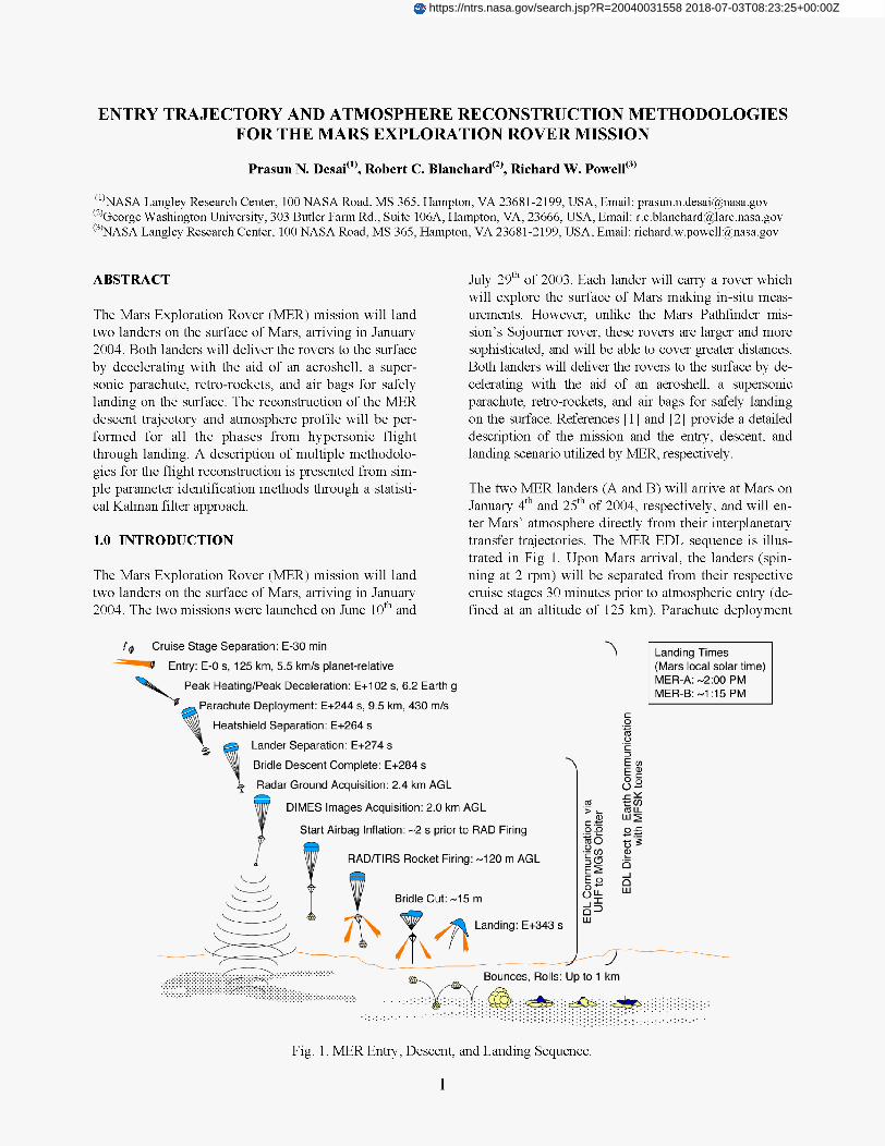
The two MER landers (A and B) will arrive at Mars on January 4* and 25* of 2004, respectively, and will en- ter Mars' atmosphere directly from their interplanetary transfer trajectories. The MER EDL sequence is illus- trated in Fig 1. Upon Mars arrival, the landers (spin- ning at 2 rpm) will be separated from their respective cruise stages 30 minutes prior to atmospheric entry (de- fined at an altitude of 125 km). Parachute deployment

' Cruise Stage Separation: E-30 min - Entry: E-0 s, 125 km, 5.5 km/s planet-relative

Peak Heating/Peak Deceleration: E+102 s, 6.2 Earth g

arachute Deployment: E+244 s, 9.5 km, 430 mls

Heatshield Separation: E+264 s

Lander Separation: E+274 s

Bridle Descent Complete: E+284 s

Radar Ground Acquisition: 2.4 km AGL

DIMES Images Acquisition: 2.0 km AGL P Start Airbag Inflation: -2 s prior to RAD Firing

-.

(Mars local solar time) MER-A: -2100 PM MER-B: -1 :15 PM

RAD/TlRS Rocket Firing: -1 20 m AGL

Bridle Cut: -15 m

Landing: E+343 s

es, Rolls: Up to 1 km

Fig. 1. MER Entry, Descent, and Landing Sequence.

1

https://ntrs.nasa.gov/search.jsp?R=20040031558 2018-07-03T08:23:25+00:00Z

is determined by the on-board flight software based on vehicle deceleration measurements obtained from two Litton LN-200 Inertial Measurement Units (IMU); one mounted in the backshell is used in conjunction with another inside the rover. Deployment is nominally tar- geted to a dynamic pressure of 700 N/m2 (occurring at approximately 244 s after entry interface) which corre- sponds to an altitude of -9.5 km. The heatshield is jet- tisoned 20 s after parachute deployment. The lander descent along its bridle is initiated 10 s thereafter. At an altitude of 2.4 km above ground level (AGL), a ra- dar altimeter acquires the ground. The radar altimeter, with its antenna mounted at one of the lower corners of the lander tetrahedron, provides distance measurements to the local surface for use by the on-board flight soft- ware to determine the solution time for firing the Rocket Assisted Deceleration (RAD) system (at -120 m AGL). Airbag inflation occurs approximately 2 s prior to RAD firing. The objective of the RAD rockets is to zero the vertical velocity of the lander -15 m above the ground. The bridle will then be cut, and the inflated airbagAander configuration freefalls to the sur- face. Sufficient impulse remains in the retrorocket motors to carry the backshell and parachute to a safe distance away from the lander.

To tolerate the presence of high near surface winds and wind shears, an additional set of three steering rockets named Transverse Impulse Rocket Subsystem (TIRS) can be fired in any combination at the time of RAD firing. In addition, at approximately 2 km AGL, the Descent Image Motion Estimation Subsystem (DIMES) estimates the horizontal velocity of the vehicle with re- spect to the surface by taking three pictures (separated by about 5 s each). This horizontal velocity measure- ment, in conjunction with data taken by the backshell and rover IMUs are used by the on-flight software to determine if any TIRS rockets should be fired.

2.0 RECONSTRUCTION APPROACH

After landing of MER-A, reconstruction of the entry is desired, not only to assess the accuracy of the pre-entry predictions to the flight data (a worthy goal in itself), but more importantly to gain confidence in this predic- tion capability for the second landing of MER-B three weeks later. This understanding is crucial in order to develop conficence in the pre-entry prediction, and in any changes that maybe proposed to assist the MER-B entry as a result of the knowledge that is ascertained from the reconstruction effort.

The reconstruction of the MER descent trajectory and atmosphere profile will be performed for all the phases

highlighted in Fig. 1 (Le., from hypersonic flight through landing). Multiple methodologies for the flight reconstruction will be applied from simple parameter identification methods through a statistical Kalman filter approach. Various reconstruction methods are employed in order to gain confidence in the overall re- construction predictions along with error assessments. The methods are described in subsequent sections.

During descent, three-axis accelerometer and gyro data will be acquired from two Litton LN-200 IMUs (one inside the backshell and another inside the rover). During the parachute descent phase, a redundant al- timeter data will supplement the accelerometer and gyro data. These data sets will be used in the recon- struction effort to determine key parameters of interest, such as, times and conditions at major descent events (e. g., parachute deployment, retro-rocket firing, land- ing position, etc.). In addition, a complete time history of the position, velocity, and entry attitude will also be produced. Furthermore, the capsule aerodynamics and parachute loads will be determined for comparison to pre-entry predictions along with refinements in atmos- phere model parameters.

3.0 DETERMINISTIC ATTITUDE METHOD

The approach that will be used for the MER attitude reconstruction from entry to parachute deployment will closely follow the attitude reconstruction effort em- ployed on Mars Pathfinder (MPF) [3]. The effort of the MPF entry attitude reconstruction was to focus on cal- culating the total angle-of-attack history to validate the MPF aerodynamic database methodology. The MPF aerodynamic database was developed using only com- putational fluid dynamics (CFD) methods. The higher MPF entry velocity required the use of CFD to extend the database beyond the Viking experience. The CFD analysis indicated two bounded instabilities for the MPF conditions that were outside the Viking flight re- gime. Due to the reliance on CFD for MPF, and all follow-on spacecraft, it was important to reconstruct the entry attitude to see if the predicted instabilities were detected. The only MPF flight data that could be used for the reconstruction was three-axis accelerome- ter data (no IMU was flown on MPF). This limited data precluded the use of many reconstruction techniques.

In general, the correspondence of measured accelera- tion and predicted aerodynamic coefficients is compli- cated by the unknown freestream density. Velocity can be derived from integrated accelerations, but density was not directly measured during the MPF descent (as is the case for MER). This complicating factor can be

2

removed by examining the ratio of normal to axial forces (FN and FA) and normal to axial aerodynamic coefficients (CN and CA):

where q is dynamic pressure, m is mass, and S is refer- ence area.

The predicted values of this normal to axial ratio for the MPF entry were calculated using the six-degree-of- freedom MPF simulation based on the Program to Op- timize Simulated Trajectories (POST) [4] code with the aerodynamic coefficients derived from the CFD analy- sis. This simulation was initialized using the initial state vector determined four hours prior to entry interface. Fig. 2 shows the comparison of the total angle-of-attack (aT) from the pre-entry simulation and that reconstructed from the flight accelerometer data utilizing this recon- struction methodology. Comparison of the data shows very good agreement and confirm the existence of the two bounded instabilities predicted by the CFD analysis.

4.1 EQUATIONS OF MOTION

Typically, the motion of an entry vehicle during de- scent and landing is obtained by integrating a system of nonlinear first-order differential equations. These dif- ferential equations account for the vehicle's motion through the atmosphere as it is attracted to the surface by the planet's gravitational field. Symbolically, the equations can be expressed as;

where x(t) is a column vector of state variables which completely describe the velocity, position, and orienta- tion of the vehicle at any given time, t.

For illustration purposes, the state x(t), written as a partitioned column vector, may include the following variables:

X = Pre-entry Simulation

6 5 -

F 4

$ 2 '03

1

0 ~

oreintation

north inertial velocity wrt areographic frame east inertial velocity wrt areographic frame down inertial velocity wrt areographic frame

radius to planet center declination longitude

quaternion mag. wrt areographic frame quaternion comp. wrt areographic frame quaternion comp. wrt areographic frame quaternion comp. wrt areographic frame

'len variables are shown for completeness, but there are 6

5 rameters have the constraint: Reconstructed Profile only 9 independent variables since the orientation pa-

- 2 2 2 2

z 4 $ 2

e,, + e, + e2 + e3 = 1

The corresponding nonlinear differential equations ex-

'03

1

0 20 40 60 80 100 120 140 160 180 pressed in terms of the state are: Time [SI

Fig. 2. MPF Entry Attitude Reconstruction Comparison.

This method of reconstruction is very fast and can pro- vide a good first-order reconstruction of the entry an- gle-of-attack and confirmation of the aerodynamic co-

tion of 2001 Mars Odyssey Orbiter atmospheric passes during the aerobraking portion of the mission, and will be utilized for MER.

efficients. This method was adapted for the reconstruc- x =

4.0 STATISTICAL METHODS

The following section describes multiple statistical ap- proaches for performing flight reconstruction.

-W i U ~

r

rc

v 0 ~-

m

3

where a,b, a,b, azb are the external accelerations (i.e., due to aerodynamic forces, thrust, etc.) in body frame coordinates and P, Q, R are angular velocities in body coordinates, Gc2b is the direction cosine matrix (DCM) for the coordinate transformation from areocentric to body axis coordinates, w is the angular velocity (as- sumed constant) of the planet, and J2 is the second zonal harmonic of the planet. The above set of differential equations is adequate to generate the trajectory provided that both body accelerations and angular rates are avail- able. For MER, accelerometer and gyro data will be taken at 8 Hz during the entry, descent, and landing.

G~~~ =

Note that,

e: + et -e; -e,’

2(e1e, - e,e,) 2(e1e, + e,e,)

2(e1e, + e,e,) e: -e: + e; -e,’

2(e,e, - e,el)

2(e1e3 - e,e,) 2(e1e, + e2e3)

e: -e: -e; + e:

where @d is the areodetic latitude, and

e , -el - e2 + e3 -sin-l[2(e1e3 - e,e2)]

Gd2b is the DCM from areodetic to body axis.

The trajectory generation process involves integrating Eq. (l), commonly referred to as the “equations-of- motion”, given a set of initial conditions (or “constants of the motion”) at some reference time to (Le., x,). As an example of exercising this methodology, Figs. 3-5 show that the state variables of the hypersonic portion of the MER entry can be reproduced very accurately utilizing simulated accelerometer and gyro data ob- tained from a MER trajectory simulation.

The velocity state variables shown in Fig. 3 are given in a local-horizontal, or areodetic frame. The position state, shown in Fig. 4, display the corresponding areo- detic position variables.

I 50 100 150 200 250

1500, I

I 50 100 150 200 250

Time [SI

Fig. 3 MER Areodetic Velocity Component Time History.

I 50 100 150 200 250

-351

Time [SI

Fig. 4 MER Areodetic Position Component Time History.

Fig. 5 shows the quaternion orientation parameters af- ter being transformed into Euler variables yaw (@), pitch (e), and roll (I)) using the following transform:

The roll rate of the MER vehicle of 12 deg/s during entry is readily seen in the top graph on Fig. 5.

4

I 50 100 150 200 250

-30

87 n n I

I 50 100 150 200 250

Time [SI

Fig. 5 MER Euler Angle (Yaw, Pitch, Roll) Time History.

4.2 MEASUREMENT EQUATIONS

Given x,, then at any given time, a set of measurements can be calculated as a function of the state variables written symbolically as;

For illustrative purposes, assume body axes accelera- tions are to be obtained during entry and descent to the surface, then the measurements equations in terms of the state variables are,

where, CA, Cy, and CN are the vehicle’s body axes aerodynamic coefficients, Sref is the corresponding ref- erence area, m is the mass (assumed constant), p is the atmospheric density, and VA is the vehicle’s relative velocity vector which can be expressed in terms of state variables as,

Simply stated, the trajectory reconstruction problem is the inverse operation of the trajectory generation proc- ess just described. That is, given measurements z,, find the initial conditions x, using Eqs. (1) and (2). Ideally, for the state variables shown, only 10 data points are needed to determine the 10 constants of the motion re-

quired to completely define the system. Realistically, however, more than 10 measurements are usually available, and each measurement is accompanied with noise (and sometime a bias). To take both of these facts into account requires some sort of a “regression” analysis. Classically, several well-developed schemes have been successfully applied to resolve the problem of handling multiple measurements in the presence of measurement uncertainty, such as, Least-Squares, Weighted Least-Squares, Batch (or Recursive) Least- Squares, Linear Kalman Filter, Extended Kalman Fil- ter, to name a few of the most applicable data process- ing schemes. Each of these regression or data process- ing schemes are statistical in nature and evolve from optimizing (minimizing or maximizing) some payoff function typically composed of the measurement re- siduals (observed minus calculated measurements). For MER, several of these filtering schemes will be applied in the trajectory reconstruction process for determining the constants of the motion. A brief review of the can- didate trajectory processing schemes is given in the subsequent sections.

4.3 LEAST-SQUARES PROCESS

The simplest measurement processing approach is the Least-Squares. Under certain conditions this processing scheme can provide an adequate solution to the trajec- tory reconstruction process. An outline of the devel- opment process is as follows.

The system dynamics equations [Eq. (l)] are linearized by truncating a Taylor series expansion about some reference trajectory, xref, that is,

df d X

6X - 6 ~ = F ( x ) ~ x (4)

where 6x = (x - xref) and F(x) is the matrix of partial derivatives of the state derivatives, or equations-of- motion (also called the “Jacobian” matrix). A solution to Eq. (4) is

6x(t) = @(t,to)6xo

where @(t, to) [called the “state transition” matrix for obvious reasons] is obtained by integrating,

starting with an initial condition, @(to,t,) = I, the iden- tity matrix. Linearizing the measurement Eq. (2) yields the measurement residuals,

5

and minimizing the sum of the squares of the residuals provides an update to the reference trajectory constants of the motion &?,as,

62, = ( A ~ A ) - ~ A ~ ~ ~

where the column vector A = G(t,)@(t,,t,). Adding 62, to x,,f provides an update to the initial reference tra- jectory. An iterative process can be developed (using root-mean-square, or other convergence criteria) to take into account linearity assumptions. Note that the statistical errors of the motion constants are readily available through the covariance matrix,

W =

The “best” estimate, or the Weighted-Least-Square cor- rection to the constant of the motion then becomes,

P = cov(x,) = ( ~ ~ ~ 1 - l 4.5 SEQUENTIAL-BATCH LEAST-SQUARES

Using this approach, the data weights are all assumed to be equal to one.

4.4 WEIGHTED LEAST-SQUARES

The Least-Squares process (filter) can be readily modi- fied to account for different measurement types with their associated “weights”, or factors of importance in obtaining a solution. This mechanism allows for giving more importance to certain select measurements. This is accomplished by introducing a weighing matrix W that contains on the diagonal the reciprocal of the squares of the measurement standard deviations. That is, for n measurement times,

0-2(ti) =

There are some well-known dlfficulties to using the Least-Squares approach to obtaining the trajectory solu- tion. One immediate difficulty is that there is no arrange- ment for incorporating the initial state errors, If avail- able. Interplanetary navigation state and their associated errors in the form of a covariance matrix are typically available at the entry interface. However, the standard Weighted-Least Squares formulation has no arrange- ment to include state errors before processing a separate set of data. This can be remedied by use of the modlfied form known as the Batch, or Recursive, or Sequential Least-Squares process discussed in the next section.

where, at each measurement time, if there are more than one type of measurement (e.g., acceleration, al- timetry, radar, etc.), then each element of the matrix can be composed of several different weighing factors. That is, at the ith measurement, assuming there are m types of measurements, then

Aside from allowing the navigation covariance to be incorporated in the entry, descent, and landing data analysis, the Sequential-Batch Least-Squares process has other additional features. One is that it is possible to keep the matrix size small by processing short batches of data, which is sometimes important, par- ticularly when dealing with a non-linear problem, such as during entry. It also is convenient for processing ad- ditional data later using an earlier converged solution without reprocessing the earlier data.

The process can be stated as follows. After k data points have been processed and converged to a solution of the constants of the motion, X,,k with the corre- sponding covariance matrix, Pk , then the best estimate correction to the state after n more data points is,

ax,, = (AT,W,A, + Pi1)-’(AT,W,6z, + AT,Wk6zk)

where the corresponding covariance matrix is:

P = (AT,w,A, + pil1-l

and the subscript “n” is the evaluation of the variable using the newly acquired data.

Probably the most serious problem for reconstruction of an entry trajectory using the Least-Squares formula- tion is that if the system model has unknown deficien- cies (e.g., incomplete atmospheric wind model) with respect to the generation of the measurements, then the converged solution will not reflect reality. This addi- tional degree of freedom (sometime referred to as

“process noise”) is incorporated in the Kalman filtering process, and is discussed in the next section.

4.6 EXTENDED KALMAN FILTER

The description of the motion of the entry vehicle dur- ing entry, descent, and landing (i.e., system model) de- scribed previously [Eq. (l)] is modified as follows,

x = f(x) + w ,

where x is a column vector of the system state para- meters that describe the system state at any given time [i.e., x=x(t)] and f(x) are nonlinear functions of the state, and w is zero-mean, random process noise such that the process-noise matrix describing the random process of the real-world system model is given as,

Q = E ( w w ~ )

where E is the expected value operator. The measure- ment equations to be used in the filter are also consid- ered nonlinear functions of the state and the ith meas- urement can be expressed as:

zi = g(xi) + vi

where z is a column vector of n measurements with v as the zero-mean random measurement noise such that the measurement-noise matrix describing the random process of the measurements for the ith measurement is given as,

Ri = E(vi vT)

That is, matrix R, contains the variances representing each measurement noise source.

A first-order approximation is used for the systems dy- namics matrix, F and the measurement matrix H, namely,

where I is the identity matrix and t, is the time of each measurement. For most applications the series is trun- cated to.

ai = I + F t i

The transition matrix @, will be used to propagate errors and to calculate the Kalman gain for the Extended Kal- man Filtering, but not in the propagation of the state.

The Riccati equations for the computation of the Kal- man gains at each measurement are as follows:

MI = @,P,.l@’, + QI : move errors to each meas- urement (with process- noise, Q,) starting with a given covariance matrix, Po

K, = M,H’(HM,H’ + RJ1 : calculate Kalman gain at each measurement (with measurement noise, R,)

PI = (I - K,H)M, : calculate errors after proc- essing each measurement

where PI is the covariance matrix for the state estimates after a measurement update (a posteriori errors), MI is the covariance matrix for the state before an update (a priori errors). These errors are calculated in the pres- ence of unknown modeling errors (represented by the process-noise matrix, Q,) and the random measurement errors or noise (represented by the matrix, R,).

The new state estimate K i is the old state estimate pro- jected forward to the measurement time, x, plus the Kalman gain at that time multiplied by the measure- ment residual (observed-compute measurement). That is,

K i = xi + Ki[zi - g(xi)]

In the Extended Kalman Filter the propagation of the state to each measurement is done directly by integrat- ing the nonlinear differential equations (as opposed to using the state transition matrix).

The state transition (or fundamental) matrix needed for the discrete Riccati equations to follow can be obtained from a Taylor series expansion as follows;

7

4.7 STATISTICAL RECONSTRUCTION PROCESS

5.0 SUMMARY

The process for the reconstruction of the MER trajecto- ries consists of a series of processing procedures. The strategy is to keep the procedures simple and flexible so that a state time-history can be generated with as few assumptions as possible. The method used for the MER mission will follow closely to the process that was used successfully on the Pathfinder program [5].

The first procedure consists of conditioning the dy- namic data (accelerometer and gyro measurements) re- ceived after the flight. This involves such processing as ordering, correcting for off-center-of-mass motion, filling data gaps, deleting data that falls outside statisti- cal bounds, and possibly data smoothing. This step is important to the development of the initial reference trajectory that will be generated by integrating the ac- celerometer and gyro data using, at first, the navigation estimates of the initial condition values and a form of the equations discussed previously. This step in the process provides a reconstructed trajectory that is inde- pendent of the atmosphere and the MER aerodynamics, although it does depend on the gravitational field. This process would complete the trajectory reconstruction if the initial conditions were known precisely. This is not likely to be the case (due to tracking errors). Thus, the altimeter and the landed position fix (if available) will be used to update the constants-of-the-motion.

The process for handling redundant data will involve both the sequential batch and the extended Kalman schemes (as verification) discussed previously. With the constants of the motion updated, the “reference tra- jectory” will be established allowing for estimates of the atmospheric state properties (free-stream density, pressure, and temperature) as an independent procedure. These will be obtained in a separate process using the well known hydrostatic and equation-of-state equations. This process does involve the MER aerodynamics data- base and will involve an iterative process. Unfortunately, reconstruction of the aerodynamic coefficients requires the knowledge of the atmosphere properties (e.g., den- sity, Mach number), which will not be available.

Upon completion of this step, both an initial trajectory and atmosphere will be available for further refinements. These refinements may include solving for some of the measurement parameters (bias, scale factors, etc.), and accounting for the terrain, and adjusting for the winds (particularly during the parachute phase of flight). These further refinements will likely occur after both MER-A and MER-B trajectories have been established.

The approach that will be utilized for the Mars Explo- ration Rover descent trajectory and atmosphere recon- struction from hypersonic flight through landing is de- scribed. Multiple methodologies for the flight recon- struction will be applied from simple parameter identi- fication methods through a statistical Kalman filter ap- proach. Various reconstruction methods are employed to develop confidence in the overall reconstruction predictions along with error assessment.

During the entry and descent, three-axis accelerometer and gyro data will be acquired, supplemented by al- timeter data. These data sets will be used in the recon- struction effort to determine key parameters of interest, such as, times and conditions at major descent events (e. g., parachute deployment, retro-rocket firing, land- ing position, etc.). In addition, a complete time history of the position, velocity, and entry attitude will also be produced. Furthermore, the capsule aerodynamics and parachute loads will be determined for comparison to pre-entry predictions along with refinements in atmos- phere model parameters.

6.0 REFERENCES

1. Roncoli, R. B. and Ludwinski , J. M., “Mission De- sign Overview for the Mars Exploration Rover Mis- sion,” AIAA Paper 2002-4823, August 2002.

2. Desai, P. N. and Lee, W. J., “Entry, Descent, and Landing Scenario for the Mars Exploration Rover Mis- sion,” Invited Paper #5, International Workshop on Planetary Probe Atmospheric Entry and Descent Tra- jectory Analysis and Sciences, Lisbon, Portugal, Octo- ber 2003.

3. Gnoffo, P. A, et al., “Prediction and Validation of Mars Pathfinder Hypersonic Aerodynamic Database,” Journal of Spacecraft and Rockets, Vol. 36, No. 3, May-June 1999, pp. 367-373.

4. Brauer, G. L., Cornick, D. E., and Stevenson, R., “Capabilities and Applications of the Program to Op- timize Simulated Trajectories (POST),” NASA CR- 2770, February 1977.

5. Spencer, D. A,; Blanchard, R. C.; Braun, R. D.; Kallemeyn, P. H.; and Thurman, S. W., “Mars Path- finder Entry, Descent, and Landing Reconstruction,” Journal of Spacecra3 and Rockets, Vol. 36, No. 3, May-June 1999, pp. 357-366.

8