Entropy as an explanatory concept and modelling tool in ...D. Koutsoyiannis, Entropy as an...

Entropy as an explanatory concept and modelling tool in hydrology

Demetris Koutsoyiannis Department of Water Resources and Environmental Engineering, Faculty of Civil Engineering, National Technical University of Athens, Greece ([email protected])

Dipartimento di Idraulica,Trasporti e StradeUniversità di Roma "La Sapienza"Roma, Italia, 1 Ottobre 2008

Presentation available online: http://www.itia.ntua.gr/en/docinfo/879/

How nature works? (my views …)

Does it ever obey power laws?Does it reflect fractals or multifractals everywhere?Does it just reflect chaos?Or is it based on a principle of self organized criticality (a cooperative behaviour, where the different items of large systems act together in some concerted way)?

{1, 2, 22}

D. Koutsoyiannis, Entropy as an explanatory concept and modelling tool in hydrology 3

Nature is parsimonious

Example of a parsimonious natural law: Dogs bark.

Examples of non-parsimonious laws:Black, white and spotted dogs bark.Dogs bark on Mondays, Wednesdays and Fridays.

{3}


Nature conserves a few quantities

Conservation laws govern the following (macroscopic) quantities:Mass (or matter);Linear momentum;Angular momentum;Energy;Electric charge.

Other quantities (e.g. temperature, velocity, acceleration) are not conserved.Conservation laws refer to closed systems that do not exchange heat and mass with the environment (in open systems there is no conservation).Mathematically, the conservation laws are formulated as equations (scalar for mass, energy and charge, vector for linear and angular momentum).


Nature loves extremes: A first example …

Why light follows the red paths from A to B (AB, ACB, ADB) and not other (the black) ones (e.g. AEB, AFB)?

The red paths are those that (a) reach the mirror and (b) form an angle of incidence equal to the angle of reflection.(True for most cases; not true

for AB; not general or parsimonious).

The red paths have minimum travel time (or length).

(Fermat’s principle –Not true for ADB).

The red paths have extreme (stationary, i.e. minimum or maximum) travel time (or length).

(True).A semi-cylindrical mirror

θ1 > θ

2

AB

C

E

D

F

{23}


The light example – no mirror

Assume that light can travel from A to B along a broken line with a break point F with coordinates (x, y). (This is not restrictive: later we can add a second, third, … break points). The travel distance is s(x, y) = AF + FB where

AF = (x – a)2 + y 2

FB = (x + a)2 + y 2

A: (-a,0)

Baa

F: (x, y)

B: (+a,0)s=1

1.251.5

1.752.0

2.252.5

2.753.0

-1.5

-1

-0.5

0

0.5

1

1.5

-1.5 -0.5 0.5 1.5x

y

Contours of the distance s(x, y)assuming a = 0.5

Line of minimum distance s(x, y) = 1Infinite points F essentially describing the same path


The light example with mirror

The mirror introduces an inequality constraint in the optimization: the point F should not be behind the mirror.Two points of local optima emerge on the mirror surface (the curve where the constraint is binding).

2

2.05

2.1

2.15

2.2

2.25

-0.25 0 0.25 0.5 0.75 1

φ/(2π)

s

Local maximum: s = 2.24

Local minimum: s = 2

Close up along the mirror

s=1

1.251.5

1.752.0

2.252.5

2.753.0

-1.5

-1

-0.5

0

0.5

1

1.5

-1.5 -0.5 0.5 1.5x

y

The mirror (radius r = 1)Local maximum: s = 2.24

Local minimum: s = 2

Global minimum: s = 1


A second example: a falling weightInitial position (t = 0, x = 0, u = 0)

Position x at time t

Floor

Quantities involvedPotential energy: V = –m g xKinetic energy: T = (1/2) m u 2 = (1/2) m (dx/dt)2

Total energy: E = T + VLagrangian: L = T – V = E – 2VAction: S = ∫ L dt

Alternative methodologies to find equations for the movement

1. Directly by integrating d 2x/dt 2 = g2. From conservation of total energy3. From minimization of action (more difficult)

All methodologies result in same solution (x = g t 2/2, u = dx/dt = g t)

Principle of least action (Hamilton’s principle –applicable both in classical and in quantum physics)From all possible motions between two points, the true motion has least action.More correct to substitute “extreme” (or “stationary”) for “least”.

x

{23}


How nature works? (synthesis)Property

She conserves a few quantities(mass, momentum energy, ….).

She optimizes a single quantity(dependent on the specific system; difficult to find what this quantity is).

She disallows some states(dependent on the specific system; maybe difficult to find).

Mathematical formulation

One equation per conserved quantity:

gi (s) = ci i = 1, …, kwhere ci constants; s the size n vector of state variables (n ≥ k, sometimes n = ∞).

A single “optimation”:

optimize f (s)

[i.e. maximize/minimize f (s)] This is equivalent to many equations (as many as required to determine s)Conversely, many equations can be combined into an “optimation”.

Inequality constraints:

hj (s) ≥ 0, j = 1, …, mIn conclusion, we may find how nature works solving the problem:

optimize f (s)s.t. gi (s) = ci i = 1, …, k

hj (s) ≥ 0 j = 1, …, m


The typical “optimizable” quantity in complex systems …… is entropy – entropie – Entropie – entropia – entropía – entropi –entrópia – entroopia – entropija – энтропия – ентропія – 熵 – エントロピー – مقياس – –אנטרופיה εντροπία.The word is ancient Greek (εντροπία, a feminine noun meaning: turning into; turning towards someone’s position; turning round andround).The scientific term is due to Clausius (1850).The entropy concept was fundamental to formulate the second law of thermodynamics.Boltzmann (1877), then complemented by Gibbs (1948), gave it a statistical mechanical content, showing that entropy of a macroscopical stationary state is proportional to the logarithm of the number w of possible microscopical states that correspond to this macroscopical state.Shannon (1948) generalized the mathematical form of entropy and also explored it further. At the same time, Kolmogorov (1957) founded the concept on more mathematical grounds on the basis of the measure theory.


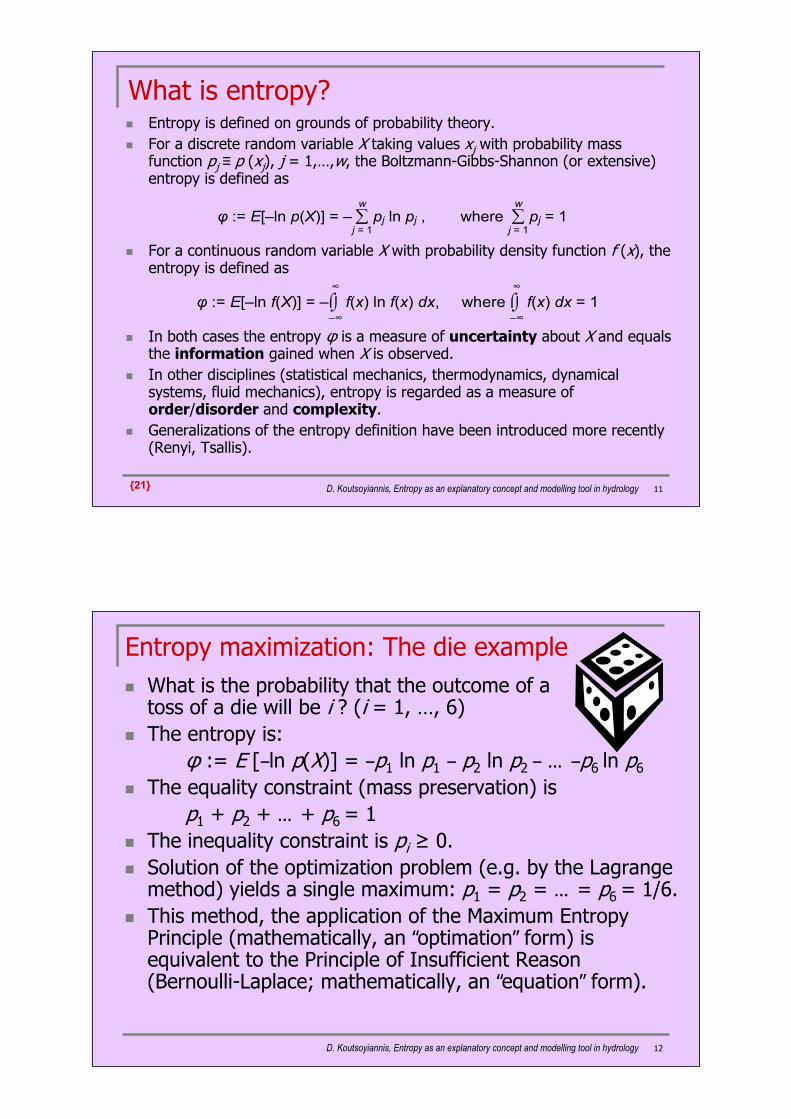
What is entropy?Entropy is defined on grounds of probability theory.For a discrete random variable X taking values xj with probability mass function pj ≡ p (xj), j = 1,…,w, the Boltzmann-Gibbs-Shannon (or extensive) entropy is defined as

For a continuous random variable X with probability density function f (x), the entropy is defined as

In both cases the entropy φ is a measure of uncertainty about X and equals the information gained when X is observed.In other disciplines (statistical mechanics, thermodynamics, dynamical systems, fluid mechanics), entropy is regarded as a measure of order/disorder and complexity.Generalizations of the entropy definition have been introduced more recently (Renyi, Tsallis).

φ := Ε[–ln f(Χ)] = –⌡⌠–∞

∞

f(x) ln f(x) dx, where ⌡⌠–∞

∞

f(x) dx = 1

φ := Ε[–ln p(Χ)] = – ∑j = 1

w

pj ln pj , where ∑j = 1

w

pj = 1

{21}


Entropy maximization: The die exampleWhat is the probability that the outcome of a toss of a die will be i ? (i = 1, …, 6)The entropy is:

φ := Ε [–ln p(Χ)] = –p1 ln p1 – p2 ln p2 – … –p6 ln p6

The equality constraint (mass preservation) isp1 + p2 + … + p6 = 1

The inequality constraint is pi ≥ 0.Solution of the optimization problem (e.g. by the Lagrange method) yields a single maximum: p1 = p2 = … = p6 = 1/6.This method, the application of the Maximum Entropy Principle (mathematically, an “optimation” form) is equivalent to the Principle of Insufficient Reason (Bernoulli-Laplace; mathematically, an “equation” form).


Entropy maximization: The loaded die example

What is the probability that the outcome of a toss of a die will be i (i = 1, …, 6) if we know that it is loaded, so that p6 – p1 = 0.2?The principle of insufficient reason does not work in this case.The maximum entropy principle works. We simply pose an additional constraint:

p6 – p1 = 0.2The solution of the optimization problem (e.g. by the Lagrange method) is a single maximum:

0

0.1

0.2

0.3

0.4

1 2 3 4 5 6i

p i FairLoaded


Entropy maximization: The temperature exampleWhat will be the temperature in my house (TH), compared to that of the environment (TE)? (Assume an open window and no heating equipment). Take a space of environment (E) in contact to the house (H) with volume equal to that of the house.Partition the continuous range of kinetic energy of molecules into several classes i = 1 (coldest), 2, …, k (hottest).Denote pi the probability that a molecule belongs to class i, and partition it to pHi and pEi, if the molecule is in the house or the environment, respectively.Form the entropy in terms of pHi and pEi .Maximize entropy conditional on pHi + pEi = pi .The result is pHi = pEi .Equal number of molecules of each class are in the house and theenvironment, so TH =TE .This could be obtained also from the principle of insufficient reason.


Is the principle of maximum entropy ontological or epistemological?

In thermodynamics and statistical physics the principle of maximum entropy is clearly ontological:

It determines (macroscopic thermodynamical) actual states of physical systems.

Jaynes (1957) introduced the principle of maximum entropy as an epistemological principle in a probabilistic context:

It is used to infer unknown probabilities from known information.The (unknown) density function f (x) of a random variable X is the one that maximizes the entropy φ, subject to any known constraints.

Are these two different principles or one? If Nature aligns itself with the (ontological) principle, why not use the same principle in logic for inference about Nature?


Formalization of the principle of maximum entropyIn both physics and logical inference, the principle of maximum entropy postulates that the entropy of a random variable should be at maximum, under some conditions, formulated as constraints, which incorporate the information that is given about this variable.Typical constraints used in a probabilistic or physical context are:

In statistical physics, if X denotes the momentum of molecules or atoms in a gas volume, the mean and variance constraints correspond precisely to the principles of preservation of momentum and energy.

⌡⌠–∞

∞

f(x) dx = 1, Ε[Χ] = ⌡⌠–∞

∞

x f(x) dx = μ

Ε[Χ 2] = ⌡⌠–∞

∞

x2 f(x) dx = σ2 + μ2, Ε[Χi Xi + 1] = ⌡⌠–∞

∞

xi xi + 1 f(xi, xi + 1) dxi dxi + 1 = ρ σ2 + μ2

Mass Mean/Momentum

Dependence/StressVariance/Energy

x ≥ 0

Non-negativity

{18, 19}


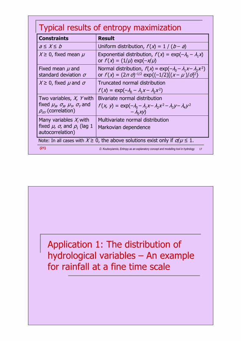
Typical results of entropy maximizationConstraints Result

a ≤ X ≤ b Uniform distribution, f (x) = 1 / (b – a)

X ≥ 0, fixed mean µ Exponential distribution, f (x) = exp(–λ0 – λ1x)or f (x) = (1/µ) exp(–x/µ)

Fixed mean µ and standard deviation σ

Normal distribution, f (x) = exp(–λ0 – λ1x – λ2x 2) or f (x) = (2π σ)–1/2 exp{(–1/2)[(x – µ )/σ]2}

X ≥ 0, fixed µ and σ Truncated normal distributionf (x) = exp(–λ0 – λ1x – λ2x 2)

Two variables, X, Y with fixed µΧ, σX, µΥ, σΥ and ρXY (correlation)

Bivariate normal distributionf (x, y) = exp(–λ0 – λ1x – λ2x 2 – λ3y – λ4y 2

– λ5xy)

Many variables Xi with fixed µ, σ, and ρ1 (lag 1 autocorrelation)

Multivariate normal distributionMarkovian dependence

Note: In all cases with X ≥ 0, the above solutions exist only if σ/µ ≤ 1.{21}

Application 1: The distribution of hydrological variables – An example for rainfall at a fine time scale


Step 1Let Xi denote the rainfall rate at time i discretized at a fine time scale (tending tozero).What we definitely know about Xi is Xi ≥ 0.Maximization of entropy with only this condition is not possible.Now let us assume that rainfall has a specified mean µ.Maximization of entropy with constraints

Xi ≥ 0, E [X ] = x f (x) dx = µ

results in the exponential distribution: f (x) = exp(–x/µ)/µ.

In addition, let us assume that there is some time dependence of Xi, quantified by E[Xi Xi + 1] = γ ; this will introduce an additional constraint for the multivariate distribution

E [Xi Xi+1] = xi xi+1 f (xi , xi+1) dxi dxi+1 = γ = ρ σ 2 + µ 2

(for the exponential distribution σ = µ and thus γ = ρ σ 2 + µ 2 = (ρ + 1) µ 2 > µ 2).

Entropy maximization in multivariate setting will result in Markovian dependence.

∫∞

∞−

∫∞

∞−∫∞

∞−

{14}


Step 2The constant mean constraint in rainfall modelling does not result from a natural principle – as for instance in the physics of an ideal gas, where it represents the preservation of momentum.Although it is reasonable to assume a specific mean rainfall, we can allow this to vary in time.In this case we can assume that the mean at time i is the realization of a random process Mi which has mean µ and lag 1 autocorrelation ρ M > ρ.Application of the maximum entropy principle will produce that Mi is Markovian with exponential distribution.Then application of conditional distribution algebra results in

f (x) = 2 K0(2 (x/µ)1/2)/µ, F (x) = 1 – 2 (x/µ)1/2 K1(2 (x/µ)1/2)/µ

where Kn(x) is the modified Bessel function of the second kind (important observation: f (0) = ∞, whereas in the exponential distribution f (0) = µ < ∞).The moments of this distribution are E [X n] = µ n n!2 (note: in exponential distribution E[X n] = µ n n!) so that

E[X] = µ, Var[X] = 3 µ2 → CV = σ/µ = √3 > 1

The dependence structure becomes more complex than Markovian (difficult to find an analytical solution).


Step 3Proceeding in a similar manner as in step 2, we can now replace the constant mean µ of the process Mi with a varying mean, represented by another stochastic process Ni with mean µ and lag 1 autocorrelation ρ N

> ρ M > ρ.In this manner we can construct a chain of processes, each member of which represents the mean of the previous process.By construction, the lag 1 autocorrelations of these processes form a monotonically increasing sequence, i.e. …. > ρ N > ρ M > ρ.The scale of change or fluctuation of each process of the chain is a monotonically increasing sequence, i.e. …. > q N > q M > q, where q := (–ln ρ)–1; the scale of fluctuation represents the time required for the process to decorrelate down to an autocorrelation 1/e.The (unconditional) mean of all processes is the same, µ.All moments except the first form an increasing sequence as we proceed through the chain; higher moments increase more.Analytical handling of the marginal distribution and the dependence structure is very difficult.However we can easily inspect the idea using Monte Carlo simulation.


A demonstration using a chain with 3 processesSimulation of a Markovian process with exponential distribution is easy and precise; there are several methodologies to implement it.Here we implement an Exponential Markov (EM) process as

Xi = µ [–ln G (Yi)]where µ is the mean, Yi is a standard AR(1) process with standard normal distribution and G ( ) is the standard normal distribution function. Simulations with a length 10 000 were performed for the following cases (for comparison).

Case 1 EM 2 EM 3 EM

Process X M X N M X

Mean 1 1 - 1 - -

0.85 0.2

0.626.2

0.25

0.72

Lag 1 autocorrelation* 0.48 0.9 0.99

Processes in chain

Scale of fluctuation 1.37 9.5 99.5

Mean 1 1 1Final process(Χ )

Standard deviation 1 1.73 3.30

Lag 1 autocorrelation 0.48 0.48 0.48

* Autocorrelation coefficients refer to the standard AR(1) process but are approximately equal in the EM process.


Simulation results – distribution function

As the number of processes in the chain increases, the right tail of the distribution moves toward higher “rainfall intensity” values and its shape changes; simultaneously the probability density becomes infinite for x = 0. The probability plot of the “3 EM” case seems to suggest a long tail (a power type law, instead of the exponential type of model “1 EM”), which in a double logarithmic plot is depicted as a constant nonzero slope (κ = 0.40) of the empirical distribution (or an asymptotic relationship of the form x ~ T κ for large x).

Logarithmicplot of “rainfall intensity” (x ) vs. empirically estimated return period T (x) := 1/F *(x) = 1/[1 – F (x)]where F (x) is the distribution function and F *(x) the exceedence probability

Slope = 0.40

0.001

0.01

0.1

1

10

100

1 10 100 1000 10000T

x

1 EM

2 EM

3 EM


0.01

0.1

1

1 10 100j

ρ j

1 EM

2 EM

3 EM

SSS

Markov

Simulation results – dependence structure

As the number of processes in the chain increases, the shape of the autocorrelation function changes from Markovian (exponential decay – short range dependence) to power type (long range dependence).The latter type is characteristic of the Hurst-Kolmogorov behaviour, which can be represented by a simple scaling stochastic process (SSS process).

Logarithmicplot of autocorrelation coefficient ρjvs. lag j

{6, 7, 12, 15}


Slope = -0.20

-0.8

-0.4

0

0.4

0.8

0 0.5 1 1.5 2log k

log σ

(k)

1 EM

2 EM

3 EM

SSS

Simulation results – variation of the aggregated process

The slope of the logarithmic plot (as k→∞) is H – 1 where H is the Hurst coefficient.The slope in the “1 EM” case is –0.5, i.e. H = 0.5, meaning no Hurst-Kolmogorov behaviour.The slope in “3 EM” is –0.20, i.e. H = 0.80, suggesting a Hurst-Kolmogorov behaviour.

Logarithmicplot of standard deviation σ (k)

of the process aggregated at scale k, vs. scale k

{6, 7, 12, 15}


0

20

40

60

80

100

0 100 200 300 400 500

i

x i

P(X ≤ 0.1) = 9%

1 EM

0

20

40

60

80

100

0 100 200 300 400 500

i

x i

P(X ≤ 0.1) = 22%

2 EM

0

20

40

60

80

100

0 100 200 300 400 500

i

x i

P(X ≤ 0.1) = 32%

3 EM

Simulation results –visual assessment

As the number of processes in the chain increases the general shape changes:

From monotony to rich patterns From steadiness to intermittency

Plots of parts of the generated time series (selected so as to include the maximum over 10 000 generated values)


Can entropy maximization be performed in a single step? (The Tsallis entropy)

A generalization of the Boltzmann-Gibbs-Shannon entropy has been proposed by Tsallis (1998, 2004)

with q = 1 corresponding to the Boltzmann-Gibbs-Shannon entropy.Maximization of Tsallis entropy with known µ yields

f (x) = [1 + κ (λ0 + λ1 x)] –1 – 1/κ, x ≥ 0

where κ := (1 – q)/q and λ0, λ1, λ2 and are parameters. Clearly, this is the Pareto distribution and has an over-exponential (power-type) distribution tail.Whilst this approach succeeds in producing a long tail to the right, it fails in reproducing the tail to the left (it underpredicts the probability of very low values).Furthermore, a single-step approach based on the Tsallis entropy cannot reproduce the Hurst-Kolmogorov behaviour.

1

)]([1

−

−=

∫∞

∞−

q

xf

φ

q

q

{10, 24, 25}


Verification of results based on real world, high resolution rainfall data

Event # 1 2 3 4 5 6 7 All Sample size 9697 4379 4211 3539 3345 3331 1034 29536Average (mm/h) 3.89 0.50 0.38 1.14 3.03 2.74 2.70 2.29St. deviation (mm/h) 6.16 0.97 0.55 1.19 3.39 2.20 2.00 4.11Coefficient of variation 1.58 1.95 1.45 1.04 1.12 0.81 0.74 1.79Skewness 4.84 9.23 5.01 2.07 3.95 1.47 0.52 6.54Kurtosis 47.12 110.24 37.38 5.52 27.34 2.91 -0.59 91.00Hurst coefficient 0.94 0.76 0.92 0.95 0.90 0.87 0.97 0.94

0

20

40

60

80

100

120

0 5000 10000 15000 20000 25000 30000

Ra

infa

ll in

ten

sity

(m

m/h

)

Event 1 Event 2 Event 3 Event 4 Event 5 Event 6 Ev 7

Plot of a high resolution (10 s) data set consisting of seven storms occurred in Iowa in 1990-91

Statistics of the seven storms and the compound record of all storms

{16}


Scaling in state

The probability plot of the compound record of all events seems to suggest a long distribution tail. In five of the seven events (1 to 5 – those with the largest durations) the variation σ/µ is higher than 1, which suggests non applicability of standard entropy theory.

-2

-1

0

1

2

3

0 1 2 3 4 5

-Log F *(x )

Log

x (

mm

/h)

Event 1 Event 2

Event 3 Event 4

Event 5 Event 6

Event 7 All events

Slope ≅ 0.3Logarithmicplots of rainfall intensity (x) vs. empirically estimated (by the Weibull formula) exceedence probability, F *(x) := 1 – F (x), for the seven events

{10, 16}


Scaling in time

Each of the events separately indicates a Hurst-Kolmogorov behaviour with Hurst coefficient ranging form 0.76 to 0.97.The Hurst-Kolmogorov behaviour is very clear in the compound record of all events, with Hurst coefficient 0.94.

Logarithmic plots of standard deviation σ (κ) of rainfall intensity vs. time scale k for the seven events and the compound record

-0.6

-0.4

-0.2

0.0

0.2

0.4

0.6

0.8

1.0

0.0 0.5 1.0 1.5 2.0 2.5 3.0 3.5Log k

Log σ

(k)

H = 0.92 (Event 3)

H = 0.76 (Event 2)

H = 0.95 (Event 4)

H = 0.97 (Event 7) H = 0.87 (Event 6)

H = 0.90 (Event 5)H = 0.94 (All)

H = 0.94 (Event 1)


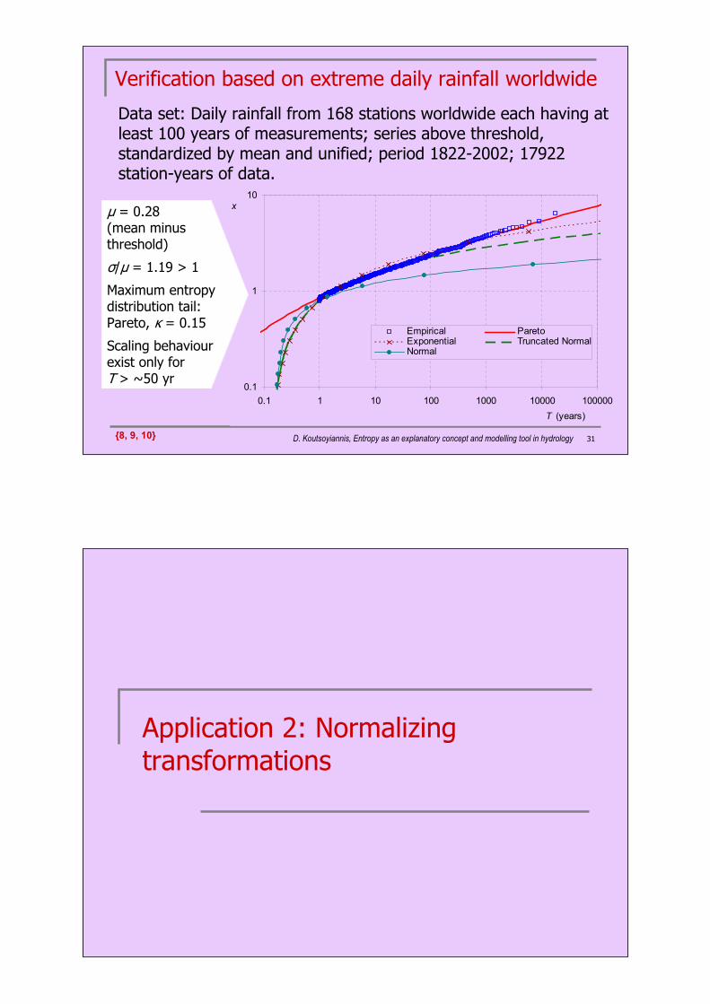
Verification based on extreme daily rainfall worldwide

Data set: Daily rainfall from 168 stations worldwide each having at least 100 years of measurements; series above threshold, standardized by mean and unified; period 1822-2002; 17922 station-years of data.

0.1

1

10

0.1 1 10 100 1000 10000 100000

T (years)

x

Empirical ParetoExponential Truncated NormalNormal

{8, 9, 10}

µ = 0.28 (mean minus threshold)

σ/µ = 1.19 > 1

Maximum entropy distribution tail: Pareto, κ = 0.15

Scaling behaviourexist only for T > ~50 yr

Application 2: Normalizing transformations


General framework

The normal distribution is very convenient in building a stochastic model.The maximum entropy framework can help establish a normalizing transformation which could preserve the distribution behaviour at its tails.When only the right tail is of interest, the following transformation (1) can result from application of the result of the Tsallis entropy maximization:

Here c is a translation parameter with same units as x, κ the tail-determining dimensionless parameter, and λ a scale parameter with same units as x, which enables physical consistency of the transformation. It is easily seen that: (a) z has the same units as x; (b) for x/λ ranging in [0, ∞), z/λ also ranges in [0, ∞ ); and (c) for κ = 0, z is identical to x. When the right tail (for x → 0) is also of interest, the following modification (2) with additional parameter α (with same unit as x) and ν (dimensionless) yields a power-type right tail for f (x) simultaneously infinitizing it for x → 0:

g (x) = ⎣⎢⎡

⎦⎥⎤

⎝⎜⎛

⎠⎟⎞xα

-ν

+ 1⎩⎨⎧ c + sgn(x – c) λ ⎝⎜

⎛⎠⎟⎞

1 + 1κ ln ⎣

⎢⎡

⎦⎥⎤

1 + κ ⎝⎜⎛

⎠⎟⎞x – c

λ

2

⎭⎬⎫

z = g (x) – g (0), g (x) = c + sgn(x – c) λ ⎝⎜⎛

⎠⎟⎞

1 + 1κ ln ⎣

⎢⎡

⎦⎥⎤

1 + κ ⎝⎜⎛

⎠⎟⎞x – c

λ

2

{17, 20}


Application to high resolution rainfall

The transformation (2) effectively transforms the observed data to normal, also implying a power type tail for X.The parameters of the transformation can be estimated by minimizing the square error of the model and the empirical distribution function.

0

20

40

60

80

100

120

-4 -2 0 2 4

Zscores

Rai

nfal

l int

ensi

ty (

mm

/h)

Observed rainfallintensity (mm/h)

-4

-3

-2

-1

0

1

2

3

4

-4 -2 0 2 4

Zscores

Tra

nsfo

rmed

rai

nfal

l int

ensi

ty (

mm

/h)

Normal distributionN(0,1)

Transformed rainfallintensity (mm/h)

{20}

Application 3: Type of dependence of hydrological processes


0

2

4

6

8

10

12

0 4 8 12 16

Monthly flow in November (km3)

Mon

thly

flo

w in

Dec

embe

r (k

m 3

)

First 78 yearsNext 53 yearsDeterministic nonlinear model

0

2

4

6

8

10

12

0 4 8 12 16

Monthly flow in November (km3)

Mon

thly

flo

w in

Dec

embe

r (k

m 3

)

First 78 yearsNext 53 yearsStochastic linear model 1Stochastic linear model 2

Modelling approaches and underlying concepts

In a deterministic approach, a relationship of any two variables (see the example in figure, referring to lagged flows of the Nile) should be described by an “exact” function which should be a non-intersecting nonlinear curve (as in the caricature case shown in the figure) passing from all points (e.g. the 78 points of the ‘fitting’ period – but the points of the ‘validation’period lie outside the curve).In a stochastic approach:

The variables are modelled as random variables.There is no need to assume an “exact” relationship. To each variable a normalizing transformation could be applied.Entropy maximization for the transformed two variables simultaneously will result in bivariate normal distribution.Bivariate normal distribution entails a linearrelationship between the two variables (Linear model 1 in figure).This explains why stochastic linear relationships are so common.Even without normalizing transformation, the dependence between two variables is virtually linear (Linear model 2 in figure).

{17}


Verification of linearity in high resolution rainfall

The figures refer to the Iowa high temporal resolution rainfall data set after normalization by transformation 2.

-4

-3

-2

-1

0

1

2

3

4

-4 -2 0 2 4

Normalized rainfall intensity at time t-1 (mm/h)

Nor

mal

ized

rai

nfal

l int

ensi

ty a

t tim

e t

(mm

/h)

-4

-3

-2

-1

0

1

2

3

4

-4 -2 0 2 4

Normalized rainfall intensity at time t-10 (mm/h)

Nor

mal

ized

rai

nfal

l int

ensi

ty a

t tim

e t

(mm

/h)

{20}

Application 4: Autocorrelation structure of hydrological processes


Entropic quantities of a stochastic processThe order 1 entropy (or simply entropy or unconditional entropy) refers to the marginal distribution of the process Xi :

The order n entropy refers to the joint distribution of the vector of variablesXn = (X1, …, Xn) taking values xn = (x1, …, xn):

The order m conditional entropy refers to the distribution of a future variable (for one time step ahead) conditional on known m past and present variables (Papoulis, 1991):

φc,m := Ε [–ln f (Χ1|X0, …, X–m + 1)] = φm – φm - 1

The conditional entropy refers to the case where the entire past is observed:

φc := limm → ∞ φc,m

The information gain when present and past are observed is:

ψ := φ – φc

Note: notation assumes stationarity.

φ := Ε[–ln f(Χi)] = –⌡⌠–∞

∞

f(x) ln f(x) dx, where ⌡⌠–∞

∞

f(x) dx = 1

φn := Ε[–ln f(Χn)] = –⌡⌠Dn

f(xn) ln f(xn) dxn

{11}


Entropy maximization for a stochastic process The minimum time scale considered is annual (to avoid periodicity).The purpose is to determine the dependence structure.The typical five constrains are used (mass/mean/variance/dependence/non-negativity).The lag one autocorrelation (used in the dependence constraint) is determined for the basic (annual) scale but the entropy maximization is done on other scales as well.The variation on annual and over-annual scales is low (σ/µ << 1) and thus the process can be approximated as Gaussian (except in tails). For a Gaussian process the n th order entropy is given aswhere δn is the determinant of the autocovariance matrix cn := Cov[Xn, Xn].The autocovariance function is assumed unknown to be determined by application of the maximum entropy principle. Additional constraints for this are:

Mathematical feasibility, i.e. positive definiteness of cn (positive δn);Physical feasibility, i.e. (a) autocorrelation function positive and (b) information gain not increasing with time scale.(Note: periodicity that may result in negative autocorrelations is not considered here due to annual and over-annual time scales).

φn = ln (2 πe)nδn

{11}


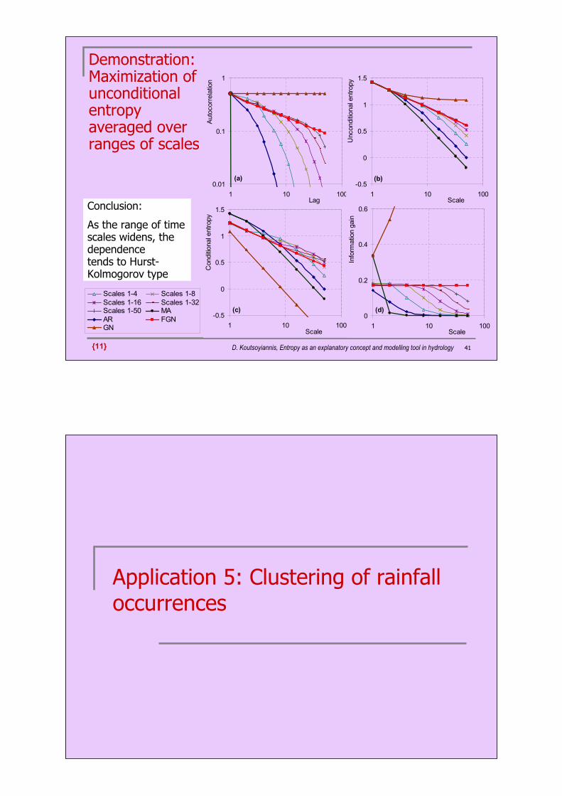
Demonstration: Maximization of unconditional entropy averaged over ranges of scales

0.01

0.1

1

1 10 100Lag

Aut

ocor

rela

tion

(a)

-0.5

0

0.5

1

1.5

1 10 100Scale

Unc

ondi

tiona

l ent

ropy

(b)

-0.5

0

0.5

1

1.5

1 10 100Scale

Con

ditio

nal e

ntro

py

(c)

0

0.2

0.4

0.6

1 10 100Scale

Info

rmat

ion

gain

(d)

Scales 1-4 Scales 1-8Scales 1-16 Scales 1-32Scales 1-50 MAAR FGNGN

Conclusion:

As the range of time scales widens, the dependence tends to Hurst-Kolmogorov type

{11}

Application 5: Clustering of rainfall occurrences


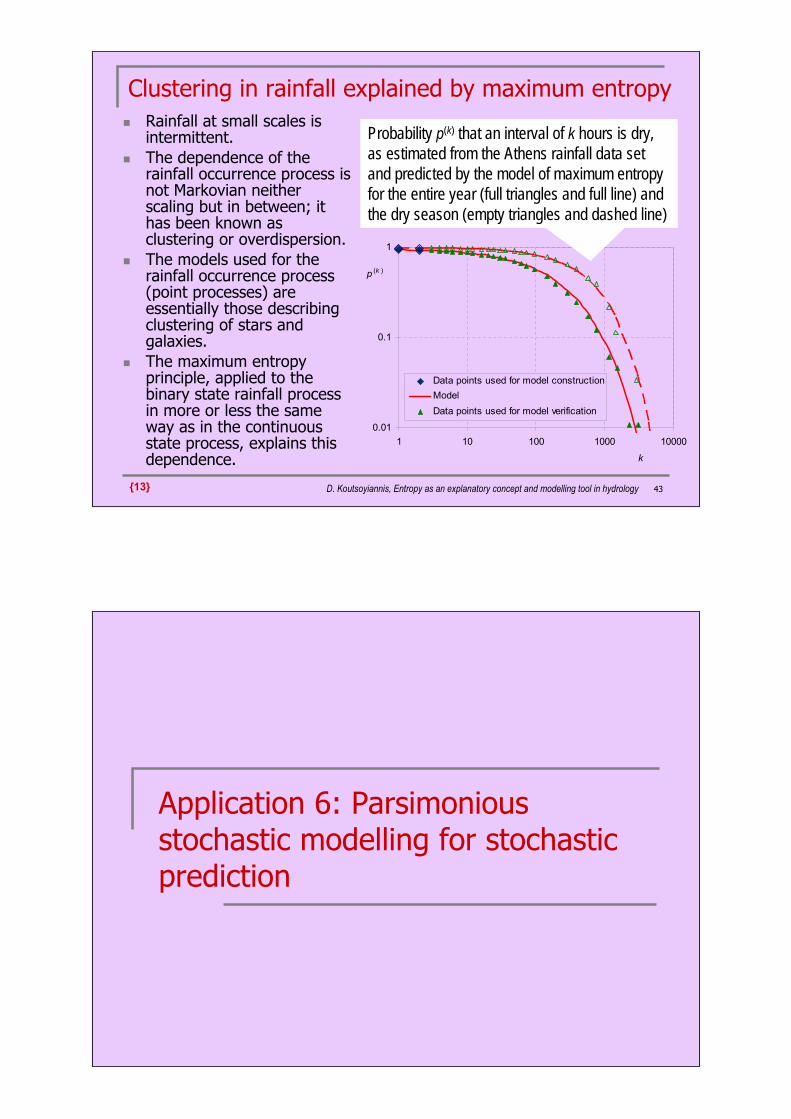
Clustering in rainfall explained by maximum entropyRainfall at small scales is intermittent.The dependence of the rainfall occurrence process is not Markovian neither scaling but in between; it has been known as clustering or overdispersion.The models used for the rainfall occurrence process (point processes) are essentially those describing clustering of stars and galaxies.The maximum entropy principle, applied to the binary state rainfall process in more or less the same way as in the continuous state process, explains this dependence.

0.01

0.1

1

1 10 100 1000 10000

k

p (k )

Data points used for model construction

Model

Data points used for model verification

Probability p(k) that an interval of k hours is dry, as estimated from the Athens rainfall data set and predicted by the model of maximum entropy for the entire year (full triangles and full line) and the dry season (empty triangles and dashed line)

{13}

Application 6: Parsimonious stochastic modelling for stochastic prediction


Stochastic model formalismThe problem of the prediction of the monthly Nile flow is studied.The prediction W of the monthly flow one month ahead, conditional on a number s of other variables with known values that compose the vector Z, is based on the linear model:

W = aT Z + Vwhere a is a vector of parameters (the superscript T denotes the transpose of a vector or matrix) and V is the prediction error, assumed independent of Z; for simplicity, all elements of Z are assumed normalized and standardized with zero mean and unit variance.For the model to take account of both long-range and short-range dependence, an optimal composition of Z was found to be the following:

All available flow measurements of the same month on previous years (78 variables = monthly flows for each of the 78 years of the calibration period).The flows of the two previous months of the same year (2 variables).

The model parameters are estimated from (Koutsoyiannis, 2000)aT = ηT h –1, Var[V ] = 1 – ηT h –1 η = 1 – aT η

where η := Cov[W, Z ] and h := Cov[Z, Z ].In forecast mode, V = 0 (to obtain the expected value of W conditional on Z = z); in simulation mode V is generated from the normal distribution independently of Z.

{4, 5, 17}


11. Parameter estimationBoth a and Var[V ] are estimated from the vector η := Cov[W, Z ] and the matrix h := Cov[Z, Z ] that contain numerous items (in our case 80 + 80 × 80 = 6480 for each month; such a number of parameters cannot be estimated from 78 monthly data values).However, most covariances in η and h depend on:

2-3 parameters (same for all months) expressing the long-range dependence, as estimated by application on the maximum entropy principle on a multi-time scale setting (a stationary component);2 parameters (per month) expressing the monthly autocovariances at the monthly scale (a cyclostationary component).

All other covariances that cannot be derived from these parameters are left ‘unestimated’ (in terms of statistics) and are calculated by the maximum entropy principle, applied on a single scale.The entropy maximization in this case has an easy analytical solution that can be formulated as a generalized Choleskydecomposition (assuming that h = b bT).

0.001

0.01

0.1

1

0 20 40 60 80

Item number

We

igh

t

Graphical depiction of the vector of weights a estimated by the maximum entropy principle for the month of July

{17}


12. Results of stochastic model (validation period)

The graphical depiction of monthly predictions in comparison to historical values, indicates good performance of the model.

0

5

10

15

20

25

30

35

Aug

-48

Aug

-50

Aug

-52

Aug

-54

Aug

-56

Aug

-58

Aug

-60

Aug

-62

Aug

-64

Aug

-66

Aug

-68

Aug

-70

Aug

-72

Aug

-74

Aug

-76

Aug

-78

Aug

-80

Aug

-82

Aug

-84

Aug

-86

Aug

-88

Aug

-90

Aug

-92

Aug

-94

Aug

-96

Aug

-98

Aug

-00

Mon

thly

flo

w (

km 3

)

Historical

Predicted

-4

-2

0

2

4

6

Aug

-48

Aug

-50

Aug

-52

Aug

-54

Aug

-56

Aug

-58

Aug

-60

Aug

-62

Aug

-64

Aug

-66

Aug

-68

Aug

-70

Aug

-72

Aug

-74

Aug

-76

Aug

-78

Aug

-80

Aug

-82

Aug

-84

Aug

-86

Aug

-88

Aug

-90

Aug

-92

Aug

-94

Aug

-96

Aug

-98

Aug

-00

Sta

ndar

dize

d m

onth

ly f

low

(km

3)

Historical

Predicted

Standardized values

Natural values

{17}


ConclusionsThe successful application of the maximum entropy principle in nature offers an explanation for of a plethora of phenomena (e.g. in thermodynamics) and statistical behaviours including:

the emergence of normal distribution (independently of the central limit theorem) in some cases;the emergence of the exponential distribution in other cases;the linearity of most stochastic laws (including the time dependence of natural processes);the scaling behaviour in state in cases with high variation (which is only a consequence of the maximum entropy principle for special cases and just an approximation, good for high return periods);the scaling behaviour in time, i.e. the Hurst-Kolmogorov behaviour;the clustering behaviour in rainfall occurrence.

All these can be interpreted as dominance of uncertainty in nature.They harmonize with the Socratic view: «Ἕν οἶδα, ὃτι οὐδέν οἶδα» (One I know, that I know nothing).This view was not a confession of modesty – Socrates regarded the knowledge of ignorance as a matter of supremacy.In this respect, the knowledge of the dominance of uncertainty can assist to better (stochastic) prediction of natural processes as well as in safer design and management of hydrosystems.


References1. Bak, P., How Nature Works, The Science of Self-Organized Criticality. Copernicus, Springer-Verlag, New York, USA, 1996.2. Buchanan, M., Ubiquity, The Science of History, or Why the World is Simpler Than We Think, Weidenfeld & Nicolson, London, 2000.3. Gauch, H. G. Jr., Scientific Method in Practice, Cambridge University Press, Cambridge, 2003. 4. Koutsoyiannis, D., Optimal decomposition of covariance matrices for multivariate stochastic models in hydrology, Water Resources Research, 35(4), 1219-

1229, 1999.5. Koutsoyiannis, D., A generalized mathematical framework for stochastic simulation and forecast of hydrologic time series, Water Resources Research,

36(6), 1519-1533, 2000.6. Koutsoyiannis, D., The Hurst phenomenon and fractional Gaussian noise made easy, Hydrological Sciences Journal, 47(4), 573-595, 2002.7. Koutsoyiannis, D., Climate change, the Hurst phenomenon, and hydrological statistics, Hydrological Sciences Journal, 48(1), 3-24, 2003.8. Koutsoyiannis, D., Statistics of extremes and estimation of extreme rainfall, 1, Theoretical investigation, Hydrological Sciences Journal, 49(4), 575-590,

2004.9. Koutsoyiannis, D., Statistics of extremes and estimation of extreme rainfall, 2, Empirical investigation of long rainfall records, Hydrological Sciences

Journal, 49(4), 591-610, 2004.10. Koutsoyiannis, D., Uncertainty, entropy, scaling and hydrological stochastics, 1, Marginal distributional properties of hydrological processes and state

scaling, Hydrological Sciences Journal, 50(3), 381-404, 2005.11. Koutsoyiannis, D., Uncertainty, entropy, scaling and hydrological stochastics, 2, Time dependence of hydrological processes and time scaling, Hydrological

Sciences Journal, 50(3), 405-426, 2005.12. Koutsoyiannis, D., Nonstationarity versus scaling in hydrology, Journal of Hydrology, 324, 239–254, 2006. 13. Koutsoyiannis, D., An entropic-stochastic representation of rainfall intermittency: The origin of clustering and persistence, Water Resources Research, 42

(1), W01401, 2006. 14. Koutsoyiannis, D., Long tails of marginal distribution and autocorrelation function of rainfall produced by the maximum entropy principle, European

Geosciences Union General Assembly 2008, Geophysical Research Abstracts, Vol. 10, Vienna, 10751, European Geosciences Union, 2008 15. Koutsoyiannis, D., and T.A. Cohn, The Hurst phenomenon and climate (solicited), European Geosciences Union General Assembly 2008, Geophysical

Research Abstracts, Vol. 10, Vienna, 11804, European Geosciences Union, 2008. 16. Koutsoyiannis, D., S.M. Papalexiou, and A. Montanari, Can a simple stochastic model generate a plethora of rainfall patterns? (invited), The Ultimate

Rainmap: Rainmap Achievements and the Future in Broad-Scale Rain Modelling, Oxford, Engineering and Physical Sciences Research Council, 2007.17. Koutsoyiannis, D., H. Yao, and A. Georgakakos, Medium-range flow prediction for the Nile: a comparison of stochastic and deterministic methods,

Hydrological Sciences Journal, 53 (1), 142–164, 2008.18. Müller, I., Entropy: a subtle concept in thermodynamics, in Entropy (edited by A. Greven, G. Keller & G. Warnecke), Princeton University Press, Princeton,

NJ, 2003.19. Müller, I., Entropy in nonequilibrium, in Entropy (edited by A. Greven, G. Keller & G. Warnecke), Princeton University Press, Princeton, NJ 2003.20. Papalexiou, S.M., A. Montanari, and D. Koutsoyiannis, Scaling properties of fine resolution point rainfall and inferences for its stochastic modelling,

European Geosciences Union General Assembly 2007, Geophysical Research Abstracts, Vol. 9, Vienna, 11253, European Geosciences Union, 2007. 21. Papoulis, A. (1991) Probability, Random Variables, and Stochastic Processes (third edn.), McGraw-Hill, New York, USA.22. Schroeder, M. R., Fractals, Chaos, Power Laws: Minutes From an Infinite Paradise, FreeMan, New York, NY, 1991. 23. Taylor, J. C., Hidden Unity in Nature’s Laws, Cambridge, 2001.24. Tsallis, C., Possible generalization of Boltzmann-Gibbs statistics, J. Stat. Phys. 52, 479-487, 1988.25. Tsallis, C., Nonextensive statistical mechanics: construction and physical interpretation, in Nonextensive Entropy, Interdisciplinary Applications (edited by

M. Gell-Mann & C. Tsallis), Oxford University Press, New York, NY, 2004.

Entropy as an explanatory concept and modelling tool in ...D. Koutsoyiannis, Entropy as an...

Documents

Transcript of Entropy as an explanatory concept and modelling tool in ...D. Koutsoyiannis, Entropy as an...