Forschungsinstitut zur Zukunft der ArbeitInstitute for the Study of Labor

DI

SC

US

SI

ON

P

AP

ER

S

ER

IE

S

Entrepreneurship in the Shadows:Wealth Constraints and Government Policy

IZA DP No. 10324

October 2016

Semih Tumen

Entrepreneurship in the Shadows:

Wealth Constraints and Government Policy

Semih Tumen Central Bank of the Republic of Turkey,

IZA and ERF

Discussion Paper No. 10324 October 2016

IZA

P.O. Box 7240 53072 Bonn

Germany

Phone: +49-228-3894-0 Fax: +49-228-3894-180

E-mail: iza@iza.org

Any opinions expressed here are those of the author(s) and not those of IZA. Research published in this series may include views on policy, but the institute itself takes no institutional policy positions. The IZA research network is committed to the IZA Guiding Principles of Research Integrity. The Institute for the Study of Labor (IZA) in Bonn is a local and virtual international research center and a place of communication between science, politics and business. IZA is an independent nonprofit organization supported by Deutsche Post Foundation. The center is associated with the University of Bonn and offers a stimulating research environment through its international network, workshops and conferences, data service, project support, research visits and doctoral program. IZA engages in (i) original and internationally competitive research in all fields of labor economics, (ii) development of policy concepts, and (iii) dissemination of research results and concepts to the interested public. IZA Discussion Papers often represent preliminary work and are circulated to encourage discussion. Citation of such a paper should account for its provisional character. A revised version may be available directly from the author.

IZA Discussion Paper No. 10324 October 2016

ABSTRACT

Entrepreneurship in the Shadows: Wealth Constraints and Government Policy*

I develop a dynamic model of forward-looking entrepreneurs, who decide whether to operate in the formal economy or informal economy and choose how much to invest in their businesses, taking government policy as given. The government has access to two policy tools: taxes on formal business activity and enforcement (or policing) discouraging informality. The main focus of the paper is on transitional dynamics under different initial wealth levels. Whether an initially small business will be trapped in the informal economy and remain small forever or grow quickly and become a large formal business depends on tax and enforcement policies. High tax rates accompanied by loose enforcement – which is mostly the case in less-developed countries (LDCs) – induce tax avoidance, discourage investment in formal businesses, and drive the entrepreneurial activity toward the informal sector even though the initial wealth level is high. Lowering taxes on formal activity joined with strict enforcement can help reducing the magnitude of poverty traps in LDCs. JEL Classification: E21, E26, L26, O17 Keywords: entrepreneurship, informal economy, government policy, investment,

wealth constraints Corresponding author: Semih Tumen Research and Monetary Policy Department Central Bank of the Republic of Turkey Istiklal Cad. No:10 06100 Ulus, Ankara Turkey E-mail: semih.tumen@tcmb.gov.tr

* I thank Tiago Cavalcanti, Enrique Martinez-Garcia, Jose Victor Rios-Rull, Mark Sanders, Orhan Torul, the participants of the Midwest Macroeconomics Meeting in Urbana, North American Summer Meeting of the Econometric Society in Los Angeles, and Econometric Society European Meeting in Gothenburg for useful suggestions. I am particularly grateful to Guido Friebel (the Editor) and two anonymous referees for their very helpful comments. The views expressed here are of my own and do not necessarily reflect those of the Central Bank of the Republic of Turkey. All errors are mine.

1 Introduction

In the developing world, informality is quite prevalent among small businesses. Using survey

data from Brazil, De Paula and Scheinkman (2011) document that around 80 percent of

the small enterprises are not registered with Brazilian tax authorities. Moreover, informal

entrepreneurs tend to invest in their businesses much less intensively than the formal ones,

which implies that formality is positively correlated with asset size.1 Similar patterns can also

be confirmed for other developing countries with large informal sectors [see Ayyagari, Beck,

and Demirguc-Kunt (2007)].

Theory predicts that high taxes on formal economic activity and loose enforcement (or polic-

ing) drive the size of informal activity up in these countries.2 The empirical evidence is in

agreement with this prediction. Both cross-country and country-level studies find that the

size of informal sector tend to be large in countries with high tax rates and weak institutional

arrangements.3 The consensus is that the government should use a mix of tax and enforcement

policies to effectively reduce the size of informal economy [Ihrig and Moe (2004)].

In this paper, I argue that wealth constraints interact with government policy to determine

the share of informal entrepreneurial activity in the economy. Specifically, I show that, given

an initial wealth level, whether a small business will be trapped in the informal economy

and stay small forever or grow quickly and establish itself as a large formal business depends

on how the government combines tax and enforcement policies. When the tax rates are

extremely high and enforcement is very loose, the extent of tax avoidance will be extensive.

Entrepreneurs with small initial wealth levels will be trapped in the informal sector forever and

the incentives to invest in physical assets will be low. Even the unconstrained entrepreneurs

(i.e., the initially wealthy ones), who initially operate formally, may tend to downsize and1Based on the information provided by SEBRAE (Brazilian Small Business Administration), small businesses account for

around 94 percent of all firms. Informal small businesses hold around 15–20 percent of the assets held by all small businessesin the Brazilian economy. Thus, the data suggest that informal small businesses tend to be much smaller than the formal ones.See De Paula and Scheinkman (2011) for more detailed descriptive statistics on formal and informal small businesses in Brazil.Throughout the paper, “size” of a small business means the “asset size.”

2See, for example, Loayza (1996), Ihrig and Moe (2004), and Tumen (2016).3Papers in this literature include Johnson, Kaufmann, and Zoido-Lobaton (1998), Schneider and Enste (2000), and Schneider,

Buehn, and Montenegro (2010). Note that some papers [e.g., Friedman, Johnson, Kaufmann, and Zoido-Lobaton (2000)] findthat the unconditional correlation between taxes and the size of informal economy can be negative; but, this negative correlationtends to turn to positive once institutional arrangements (such as enforcement and measures to combat corruption) are controlledfor.

2

switch to informality in the long run. Suppose that the government starts decreasing taxes

and tightening enforcement. At the beginning, the unconstrained entrepreneurs will exhibit a

behavioral change: they will invest in their businesses, start growing, and stay in the formal

sector forever. There will still be many small businesses trapped in the informal economy.

But, at least, informal and formal businesses coexist in the long run. When the taxes are

reduced sufficiently and enforcement is tightened further, even those informal entrepreneurs

with very low initial wealth levels may choose to grow aggressively and establish a permanent

presence in the formal economy.

The theoretical framework features a fundamental non-convexity that leads to a dual structure

in the economy: the entrepreneurs operate either in the formal economy or in the informal

economy. On the one hand, operating in the formal economy is attractive because a unit of

physical asset produces a larger amount of output in the formal economy [Thomas (1992)].

Formal activity is more costly, on the other hand, because a formal business should register

with the official tax system, but the informal business pays the tax only if it is caught.

As a result, the entrepreneur faces a cost-benefit tradeoff on the margin of formality versus

informality. This margin is the source of the fundamental non-convexity. It is well-known that

such non-convexities pave the way for poverty traps in economic models.4

In this paper, the term “poverty trap” is used to describe the extent of the “non-convergence”

problem [see Azariadis (1996)].5 In standard models, a convergence path refers to the footsteps

of the poor on the way to getting rich. However, this convergence path might be interrupted

for several reasons leading the poor to stay poor for a long time. This paper suggests that

the interactions between initial wealth levels and government policy might generate such an

interruption. To be specific, if taxes on formal economic activity is too high and enforcement

is loose, then initially wealth-constrained entrepreneurs might get trapped in the informal

4See Banerjee (2004) for an excellent review of the related literature. It is worthwhile to note that this type of non-convexitiesare sufficient but not necessary to generate poverty traps in economic models [Mookherjee and Raj (2002)].

5Note that there are also more objective/quantitative measures to define a poverty trap. For example, time series evolution ofinequality measures (i.e., the Gini index) may be used to quantify the persistence of inequality in a country and, therefore, maybe proposed as an objective measure of poverty traps. It is also possible to construct ratios of consumption on the upper versuslower portions of the income distribution and link the persistence of this measure to poverty traps. Another approach might beto compare the labor income processes of the poor and the rich to identify the factors that might lead to persistent differences inlong-run income and use those factors as objective measures of poverty traps.

3

economy and stay small forever. The “magnitude” of the poverty trap is higher if a larger

fraction of the entrepreneurs are trapped in the informal sector.6 The mechanics of poverty

trap developed in this paper are similar to the ones offered by papers including Galor and

Ryder (1989), Murphy, Shleifer, and Vishny (1989), and Durlauf (1993). This literature

suggests that differences in initial conditions—determined by history and inheritance—might

lead to non-convergence. Different from this literature, I say that government policy may

also contribute to convergence (or non-convergence) experiences and, therefore, affect the

magnitude of poverty traps.

The main contribution of this paper is the idea that the government, by setting high tax

rates on formal activity and imposing loose enforcement, can itself cause large and persistent

poverty traps. There are other theoretical papers in the literature—see, for example, Ihrig

and Moe (2004)—arguing that high tax rates joined with weak enforcement can inflate the

scale of informal activity. My paper is different from these models in two main respects.

First, the models in the literature typically compare the steady state outcomes under different

government policy scenarios, whereas the model I develop is capable of producing analytically

tractable transitional dynamics. Using the transitional dynamics exercise, one can test the role

of government policy on transitions from informality to formality or vice versa. Second, the

steady state outcomes in this literature—as in Ihrig and Moe (2004)—feature either an entirely

informal economy or an entirely formal economy depending on taxes and enforcement. The

model I develop allows for the possibility of multiple equilibria in which informal and formal

entrepreneurs can coexist in the long run. These two aspects together allow for studying

the potential interactions between government policy and the magnitude of poverty traps in

developing economies.

Although the choice of formality versus informality is a static problem, the model is built

on a basic dynamic equilibrium framework, in which the entrepreneur chooses how much

to consume and how much to invest in physical capital at each time period. In terms of the

modeling practices, the model is most closely related to Buera (2008). Similar to Buera (2008),

6See McKenzie and Woodruff (2006) for a similar definition and related literature review.

4

I show that initial wealth positions determine both the transitional dynamics and steady-state

outcomes of individuals. Different from Buera’s model, I focus on the informal versus formal

sector choice, since the main purpose of the present study is to understand the effect of

government policy on the formal/informal decision margin. Another closely related paper is

De Paula and Scheinkman (2011), who construct a static model to differentiate the informal-

formal margin using the differences in the cost of financing. Unlike their work, I specify

a fully dynamic model and focus on transitional dynamics to understand how government

policy mediates the correlation between initial wealth constraints and informal versus formal

entrepreneurship. The benchmark model assumes that the entrepreneurs have no other income

besides their revenue. They run their businesses by choosing the optimal level of assets

to employ, while labor is assumed away for simplicity. Different types of taxes that the

entrepreneur faces are represented by a single tax rate. The entrepreneurs live in a world with

perfect certainty. And, finally, the tax revenues are subject to wasteful spending. I argue

that relaxing these simplifying assumptions does not alter the qualitative predictions of the

benchmark model significantly [see Section 4].

This paper is also related to the growing body of literature on the link between entrepreneur-

ship and wealth constraints. A particular strand of this literature argues that wealth con-

straints are important determinants of entrepreneurship [see, e.g., Evans and Jovanovic (1989),

Holtz-Eakin, Joulfaian, and Rosen (1994), Blanchflower and Oswald (1998), Lindh and Ohls-

son (1998), and Gentry and Hubbard (2004)].7 I argue that wealth constraints also bind for

the intensive margin of entrepreneurial choice (i.e., choosing whether to operate as an informal

or formal entrepreneur), rather than only the extensive margin. I also argue that the degree

to which the wealth constraints bind is a function of the tax and enforcement policies, which

is a novel idea in the literature.

It is also possible to link this paper to the literature investigating how entrepreneurial saving

or investment behavior is affected by government policy. For example, Fossen and Rostam-

7Whether the correlation between wealth constraints and the probability of becoming an entrepreneur is spurious or not is acontroversial issue. See de Meza and Southey (1996), de Meza (2002), Hurst and Lusardi (2004), Nanda (2010), and Kerr andNanda (2011) for a review of the relevant issues in this literature.

5

Afschar (2012) argue that changes in government policy that entail greater income uncertainty

may lead to changes in the saving behavior of entrepreneurs via shifting both the amount and

the composition of their savings. Cullen and Gordon (2007) show using the U.S. data that

the entrepreneurial risk-taking behavior responds different forms of tax/incentive policies in

differing degrees.8 Peck (1989) argues that the design of tax policy can play important roles for

smoothing out the negative effects of market imperfections on the profits of small businesses.

Boadway, Marchand, and Pestieau (1991) derive an optimal linear tax formula and study how

it interacts with entrepreneurial choices. Similar to these papers, I also link government policy

to entrepreneurs’ choices and outcomes. Different from them, I focus on the formal/informal

margin, and show how the interactions between initial wealth constraints and government

policy determine long-run fractions of formal and informal entrepreneurs in an economy.

Although the current paper mostly adopts a developing country perspective, the link be-

tween entrepreneurship and economic growth is a source of major debate also in developed

countries. The slowdown in global economic growth rates, which became more evident fol-

lowing the 2008 financial crisis, is often argued as being a consequence of the slowdown in

productivity growth. There are several studies, including Haltiwanger, Jarmin, and Miranda

(2013), Decker, Haltiwanger, Jarmin, and Miranda (2014), and IMF (2016), linking produc-

tivity growth to entrepreneurship. So, the observed slowdown in business start-up rates in

major economies, including the U.S., Canada, and many European countries, is seen as a

major reason behind the decline in global growth rates. For example, Haltiwanger (2012)

documents that around 20 percent of the U.S. gross job creation can be attributed to busi-

ness start-ups. The picture in developing economies is somewhat different. Schoar (2010)

and Hsieh and Klenow (2014) show that there are too many entries in developing countries,

which results in too many subsistence (and potentially informal) entrepreneurs. As Decker,

Haltiwanger, Jarmin, and Miranda (2014) argue, the common element in these two examples

is the lack of high-growth transformational entrepreneurs. This paper shows that government

policy in the form of tax and enforcement incentives has a potential to increase the share of

8See also Kanbur (1981) for a general equilibrium model investigating the implications of government policy for entrepreneurialrisk taking.

6

transformational entrepreneurs and spur economic growth, which applies to both developing

and developed economies.9

Finally, it will perhaps be useful to discuss from a broader perspective the position of the cur-

rent paper within the informality literature. Informal businesses are analyzed in the literature

along three different frameworks [La Porta and Shleifer (2008, 2014), Jones (2008)]. The first

is called the “romantic view” and it suggests that informal businesses are not less produc-

tive/efficient than the formal businesses. According to this view, the informal activity is held

back by government through high taxes, strict enforcement, and weak intellectual property

rights [see, e.g., De Soto (1989, 2000)]. The key assumption, which is often criticized as being

over-optimistic, is that informal businesses are similar to formal ones, but their activity is

kept down by policy. The second is called the “parasitic view” and is less optimistic than

the romantic view. It basically says that unofficial businesses are much less productive than

their official counterparts and they are owned by less skilled entrepreneurs; thus, to stay alive,

they need to stay small and cut their prices, which harms the official productive businesses

and erodes their growth potential [see, e.g., Farrell (2004)]. The third is called the “dualistic

view,” which assumes that the economy is characterized within a dual structure that sorts

less skilled entrepreneurs to small and informal businesses and more skilled ones to large and

formal businesses [see, e.g., Rauch (1991) and Amaral and Quintin (2006)]. Along the devel-

opment path, productive resources increase and the share of formal activity goes up over time.

Eventually, the developed economy emerges with only a tiny share of informal activity. Based

on this view, the government can intervene to speed up the transition process. This paper

perfectly fits into the dualistic view and argues that government policy can increase the speed

of development through several channels. Our results on poverty traps are also consistent with

this view.

The plan of the paper is as follows. Section 2 presents the benchmark model and outlines the

solution method. Section 3 provides an extensive discussion of the transitional dynamics in

the benchmark economy. How the transitional dynamics respond to changes in government

9For other breakthrough papers linking entrepreneurship to tax policy, see Gordon (1998), Hubbard and Gentry (2000), andHubbard and Gentry (2005).

7

policy is also discussed in depth. Section 4 sketches several extensions of the benchmark model

and argues how the predictions of the benchmark model could change upon relaxing its main

assumptions. Section 5 concludes.

2 The Benchmark Model

Time is continuous and indexed by t ≥ 0. At each point in time, the entrepreneur has the

option to operate in the formal economy or informal economy. He holds physical assets a and

fully invests these assets into his business to produce output. Moreover, he chooses the level

of investment each period and add the invested amount over the stock of physical assets to be

used in production in the next period. The initial level of physical assets, a(0), is endowed to

the entrepreneur. Borrowing or lending is not allowed.

The government designs tax and enforcement policies to encourage formal economic activity.

Specifically, the government sets a tax rate as a fraction τ ∈ [0, 1] of entrepreneurial output.

The formal entrepreneur pays this fraction fully, but the informal entrepreneur pays it only if

he is caught. The probability of getting caught is described by φ ∈ [0, 1].10 This is called the

enforcement (or policing) parameter. Thus, each period the informal entrepreneur expects to

pay the tax φτ , which means that he pays the tax conditional on getting caught. This policy

setup is similar to Ihrig and Moe (2004) and Tumen (2016).

2.1 Preferences

The entrepreneur’s preferences over consumption profiles are defined by the following utility

specification:

U(c) =

∫ ∞0

e−ρtc(t)1−σ

1− σdt, (2.1)

10In the benchmark model, the parameter φ is assumed to be fixed, which means that each entrepreneur has an equal andconstant probability of getting caught by the police in the case of informal operation. But, in reality, larger businesses are muchmore visible and the probability of getting caught goes up with the asset size. To obtain an analytically solvable dynamic system,I assume that φ is fixed. But, this is relaxed later in the paper [see Section 4.1] and an extensive discussion is provided toemphasize that having φ as an increasing function of the asset size does not alter the qualitative nature of the results obtainedfrom the benchmark model.

8

where ρ is the rate of time preference and σ is the reciprocal of the intertemporal elasticity

of substitution. The constant relative risk aversion (CRRA) specification ensures that the

period utility over consumption is strictly increasing and strictly concave. It is also possible

to attribute a life-cycle interpretation to this setup. Under this interpretation, ρ = ρ∗ + d,

where ρ∗ is the rate of time preference and d is the constant rate of death for the entrepreneur.

For notational simplicity, I will abstract from life-cycle considerations and use ρ as the rate of

time preference.

2.2 Technology and Constraints

At any point in time, the physical assets of the individual entrepreneur evolve according to

the law of motion

a(t) = Y(a(t)

)− c(t), (2.2)

for all t ≥ 0 and given an initial asset level a(0) > 0. The notation a refers to the time deriva-

tive. Depreciation is assumed away. The function Y describes the net-of-tax entrepreneurial

revenue and is formulated as follows:

Y(a(t)

)=

θa(t)αf (1− τ)− s, if operates formally,

θa(t)αi(1− φτ), if operates informally,(2.3)

where 0 < αf < 1 is the returns to scale parameter in the formal economy, 0 < αi < 1 is

the returns to scale parameter in the informal economy, s > 0 is a constant social security

contribution by the formal entrepreneur, and θ > 0 is a fixed technology shifter.11 Note that

the production function θa(t)αk , k = f, i, is strictly increasing in a(t) and satisfies the standard

Inada conditions. To capture the fact that production in the formal economy is more capital

intensive than that in the informal economy, I assume αf > αi. This assumption makes formal

economy more attractive, because one unit of the physical asset produces a larger amount of

output in the formal economy than in the informal economy everything else equal. This implies11Imposing the assumption s > 0 only implies that the entrepreneur chooses to stay informal at very low asset levels. However,

it is possible to set the social security contribution s to be equal to zero without affecting any of the results qualitatively. Forsimplicity, I ignore any potential future benefits of current social security contributions to the formal entrepreneur. So, in thecurrent setup, s serves only as an arbitrary fixed cost.

9

that the entrepreneur’s sectoral choice problem is subject to a fundamental tradeoff: whether

to operate in the more productive formal economy or in the less costly (due to lower taxes) in

the informal economy.12 Note that this assumption is not critical and can be relaxed without

changing the main predictions of the benchmark model qualitatively [see Section 4.2].

2.3 Sectoral Choice

The sectoral choice problem of the entrepreneur is a static one. Given the physical asset level

a(t), the entrepreneur decides at each instant whether to operate in the formal economy or in

the informal economy based on the following choice rule:

max{θa(t)αf (1− τ)− s, θa(t)αi(1− φτ)

}. (2.4)

There exists a threshold level aT , which is time independent, making the entrepreneur in-

different between operating in the formal versus informal economy. Formally, this threshold

satisfies the following condition:

θaαf

T (1− τ)− s = θaαiT (1− φτ). (2.5)

At any instant t ≥ 0, the entrepreneur operates in the formal economy if a(t) > aT and he

operates his business in the informal economy if a(t) ≤ aT . This defines the optimal sectoral

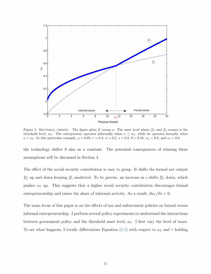
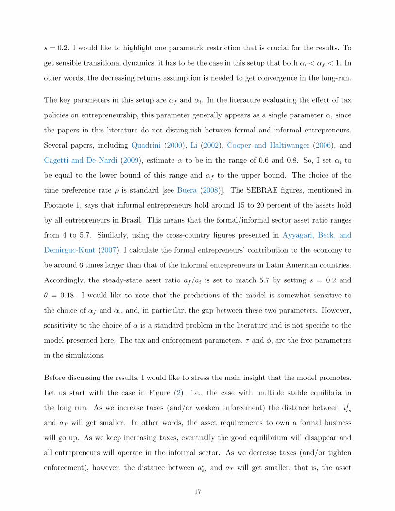
decision. Figure (1) visually describes the threshold-crossing behavior.

Notice that the threshold physical asset level aT can be redefined as the implicit function

aT (τ, φ, s, αf , αi); that is, the threshold separating formality from informality is a function of

tax/enforcement policies, technology, and the social security contribution. Throughout this

section, I assume that αf > αi and I will take those parameters fixed. Similarly, I treat

12The assumption that formal sector is more productive than the informal sector, e.g., αf > αi, has an empirical background.One can think of various reasons that may lead to this productivity gap. First, informal businesses tend to stay small to reducethe probability of getting caught. This may lead to a failure to achieve the economies of scale and the associated decline inmarginal costs. For example, WorldBank (2005) documents that a percentage point increase in the share of informal employees ina firm is associated with a 0.3 percent decline in factor productivity. Second, and related to the first, the tendency to stay smallleads the small informal businesses to hire low-skill workers, which may reduce productivity further [McKinsey (1998)]. Third,the organizational design is more inefficient in informal businesses. Fourth, access to governmental resources and legal servicesare highly restricted in the informal sector. Finally, these limited access may lead to a greater incentive for intra-organizationalcorruption.

10

0 2 4 6 8 10 12 14 16 18 20−0.2

0

0.2

0.4

0.6

0.8

1

1.2

Physical Assets

aT

Yf

Y i

Y

Informal sector Formal sector

Figure 1: Sectoral choice – The figure plots Y versus a. The asset level where Yf and Yi crosses is thethreshold level, aT . The entrepreneur operates informally when a ≤ aT , while he operates formally whena > aT . In this particular example, ρ = 0.05, τ = 0.4, φ = 0.2, s = 0.2, θ = 0.18, αf = 0.8, and αi = 0.6.

the technology shifter θ also as a constant. The potential consequences of relaxing these

assumptions will be discussed in Section 4.

The effect of the social security contribution is easy to grasp. It shifts the formal net output

Yf up and down keeping Yi unaltered. To be precise, an increase in s shifts Yf down, which

pushes aT up. This suggests that a higher social security contribution discourages formal

entrepreneurship and raises the share of informal activity. As a result, ∂aT/∂s > 0.

The main focus of this paper is on the effects of tax and enforcement policies on formal versus

informal entrepreneurship. I perform several policy experiments to understand the interactions

between government policy and the threshold asset level, aT . I first vary the level of taxes.

To see what happens, I totally differentiate Equation (2.5) with respect to aT and τ holding

11

everything else constant. This exercise yields the expression

daTdτ

=aαf

T − φaαiT

αfaαf−1T (1− τ)− αiaαi−1

T (1− φτ)> 0, (2.6)

which means that higher tax rates (everything else constant) increase the asset threshold,

discourage formal activity, and induce tax avoidance. The numerator is clearly positive. After

some algebra, it is also clear that the denominator is also positive. In other words, higher tax

rates are associated with larger physical asset requirements to operate in the formal economy.

Notice that this derivative is a function of the enforcement rate. The effect of taxes on the

threshold asset level aT will get smaller as the enforcement rate φ goes up. This means

that the policy strategy of reducing taxes to discourage informality will be more effective in

environments with weak enforcement.

Now I vary the enforcement parameter, which gives

daTdφ

=−τaαi

T

αfaαf−1T (1− τ)− αiaαi−1

T (1− φτ)< 0. (2.7)

This suggests that increasing the intensity of policing in the economy reduces the asset thresh-

old, generating a switch from informal activity toward formality. The derivative of aT with

respect to φ is a decreasing function of τ , meaning that strong enforcement will be more

efficient in low tax environments. To summarize, high taxes combined with loose policing

strongly discourage formality, while low taxes with strong enforcement reduce tax avoidance

and increase formal participation. Notice that lowering taxes in an environment with loose

policing will be an inefficient policy move. Similarly, strengthening enforcement in an envi-

ronment with high tax rates will again be inefficient. This framework suggests that the best

policy option is to strengthen enforcement while reducing taxes.

It will perhaps be useful to reemphasize the main insights gained in this static model. This

model implicitly defines the sectoral choice problem of the entrepreneur as a function of gov-

ernment policy. Lowering taxes and tightening enforcement measures can reduce the share of

informal entrepreneurship. The reason is that lower taxes reduce the cost of formality and

12

stricter regulation makes it harder to lurk in the shadows. However, the key components of

this problem, which are missing in the static sectoral choice decision, are asset accumulation

and the associated initial wealth constraints. These components determine whether a small

informal entrepreneur can end up in the formal economy in the long-run equilibrium or not.

The next subsection introduces the asset accumulation problem and describes the solution of

the fully dynamic system. This setup will enable us to understand the effect of wealth con-

straints on sectoral entrepreneurial allocation and to examine how government policy diffuses

into this relationship.

2.4 The Optimization Problem

The entrepreneur makes three choices: consumption, physical assets (i.e., investment), and

whether to operate in the formal versus informal economy. Formally, the entrepreneurs solves

the problem

maxc(t),a(t)≥0

∫ ∞0

e−ρtc(t)1−σ

1− σdt

subject to

a(t) = Y(a(t)

)− c(t),

Y(a(t)

)= max

{Yf(a(t)

),Yi(a(t)

)},

given a(0) > 0. The full solution to the static sectoral choice problem is described in detail in

the previous subsection. Taking as given government policy, the dynamic problem of choos-

ing optimal sequences of consumption and physical assets can be solved by constructing the

following current-value Hamiltonian:

H(a, λ, c, t) =c1−σ

1− σ+ λ[Y(a)− c

], (2.8)

where λ is the shadow price (or the co-state variable) used to value increments to physical

assets. To simplify the notation, I drop the time index in what follows. The first-order

13

condition with respect to consumption is simply

c−σ = λ. (2.9)

The shadow price evolves according to the law of motion

λ =

ρλ− λαfθaαf−1(1− τ), if operates formally (i.e., a > aT ),

ρλ− λαiθaαi−1(1− φτ), if operates informally (i.e., a ≤ aT ),(2.10)

where the decision to operate formally versus informally is determined by the simple threshold

aT . Using this law of motion for the co-state variable joined with the first-order condition

(2.8), the Euler equation (or the growth rate of consumption) can be formulated as

c

c=

[αfθa

αf−1(1− τ)− ρ]/σ, if a > aT ,[

αiθaαi−1(1− φτ)− ρ

]/σ, if a ≤ aT .

(2.11)

Finally, to guarantee convergence in the dynamic model, the following transversality condition

needs to be satisfied:

limT→∞

∫ T

0

e−ρtλ(t)a(t)dt = 0.

This solution suggests that there are two different consumption and asset accumulation pat-

terns in the economy: one for the formal entrepreneurs and the other for the informal en-

trepreneurs. The steady-state levels of consumption and physical assets can easily be solved

analytically. I am interested in a particular solution, in which c = 0 and a = 0. In the formal

economy, the steady-state levels of consumption and physical assets are

cfss = θ(1− τ)

[ρ

αfθ(1− τ)

]αf/(αf−1)

− s, afss =

[ρ

αfθ(1− τ)

]1/(αf−1)

, (2.12)

respectively. In the informal economy, these quantities can be expressed in a similar manner

14

as

ciss = θ(1− φτ)

[ρ

αiθ(1− φτ)

]αi/(αi−1)

, aiss =

[ρ

αiθ(1− φτ)

]1/(αi−1)

. (2.13)

Next I study transitional dynamics in this economy. The non-convexities due to sectoral

choice problem generate a potential for multiple stable equilibria at the steady state. The

government policy will determine the number and nature of these equilibrium solutions.

3 Transitional Dynamics and Government Policy

This section characterizes the co-evolution of consumption and physical asset levels, given ini-

tial conditions on individual wealth. From now on, it makes sense to assume that entrepreneurs

are heterogeneous in terms of the initial asset levels they hold. In case of multiple equilib-

ria (one for formal activity and the other for informal activity), these initial positions will

determine which equilibrium the entrepreneur converges to. Following the convention in the

analysis of dynamic models in continuous time, I will proceed with a description of the transi-

tional dynamics using a standard phase diagram over the two-dimensional asset-consumption

(a− c) space.

Two equations describe the optimal trajectories. The first equation sets c = 0 in Equation

(2.11), e.g., in the Euler equation. This equation (i.e., the c = 0 locus) is a vertical line crossing

the x-axis at the steady state asset level. On the right of this vertical line, consumption is

decreasing and it is increasing on the left. The second equation sets a = 0 in Equation (2.2),

e.g., in the law of motion for the accumulation of physical assets. This equation gives us a

set of points over which the consumption equals output minus investment at the steady state.

Above this line, asset accumulation is negative and it is positive below.

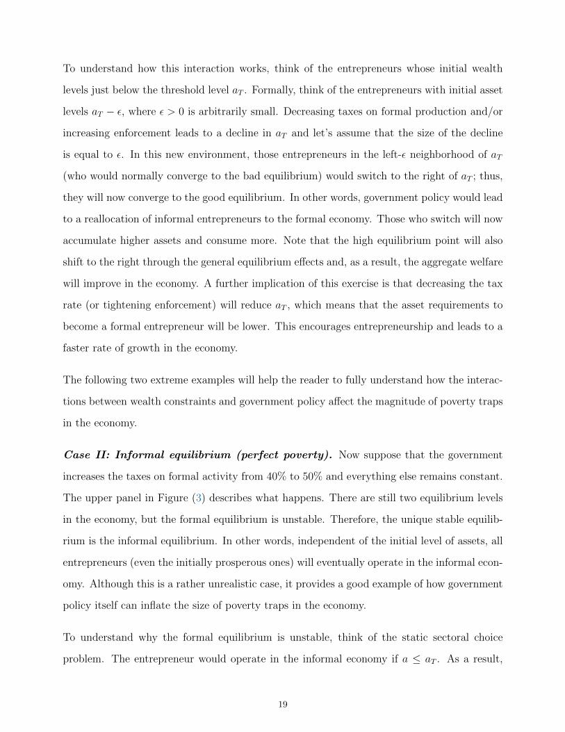
Figure (2) exemplifies a case in which there are multiple stable equilibria and separate tran-

sitional dynamics that operate below and above the asset threshold aT . In this particular

example, there are multiple stable equilibria: one for informal activity (the left of aT ) and

the other for formal activity (the right of aT ). One of this equilibria is reached conditional

15

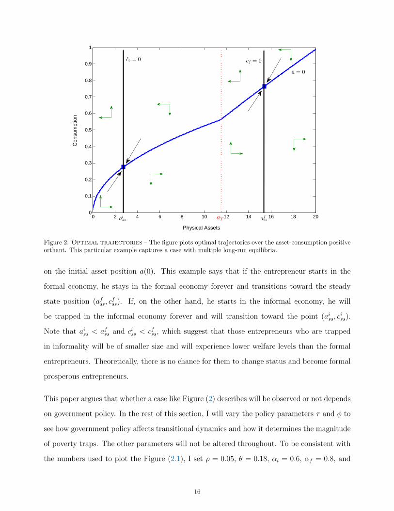
0 2 4 6 8 10 12 14 16 18 200

0.1

0.2

0.3

0.4

0.5

0.6

0.7

0.8

0.9

1

Physical Assets

aT

ci = 0 cf = 0

a= 0

afssaiss

Con

sum

ptio

n

Figure 2: Optimal trajectories – The figure plots optimal trajectories over the asset-consumption positiveorthant. This particular example captures a case with multiple long-run equilibria.

on the initial asset position a(0). This example says that if the entrepreneur starts in the

formal economy, he stays in the formal economy forever and transitions toward the steady

state position (afss, cfss). If, on the other hand, he starts in the informal economy, he will

be trapped in the informal economy forever and will transition toward the point (aiss, ciss).

Note that aiss < afss and ciss < cfss, which suggest that those entrepreneurs who are trapped

in informality will be of smaller size and will experience lower welfare levels than the formal

entrepreneurs. Theoretically, there is no chance for them to change status and become formal

prosperous entrepreneurs.

This paper argues that whether a case like Figure (2) describes will be observed or not depends

on government policy. In the rest of this section, I will vary the policy parameters τ and φ to

see how government policy affects transitional dynamics and how it determines the magnitude

of poverty traps. The other parameters will not be altered throughout. To be consistent with

the numbers used to plot the Figure (2.1), I set ρ = 0.05, θ = 0.18, αi = 0.6, αf = 0.8, and

16

s = 0.2. I would like to highlight one parametric restriction that is crucial for the results. To

get sensible transitional dynamics, it has to be the case in this setup that both αi < αf < 1. In

other words, the decreasing returns assumption is needed to get convergence in the long-run.

The key parameters in this setup are αf and αi. In the literature evaluating the effect of tax

policies on entrepreneurship, this parameter generally appears as a single parameter α, since

the papers in this literature do not distinguish between formal and informal entrepreneurs.

Several papers, including Quadrini (2000), Li (2002), Cooper and Haltiwanger (2006), and

Cagetti and De Nardi (2009), estimate α to be in the range of 0.6 and 0.8. So, I set αi to

be equal to the lower bound of this range and αf to the upper bound. The choice of the

time preference rate ρ is standard [see Buera (2008)]. The SEBRAE figures, mentioned in

Footnote 1, says that informal entrepreneurs hold around 15 to 20 percent of the assets hold

by all entrepreneurs in Brazil. This means that the formal/informal sector asset ratio ranges

from 4 to 5.7. Similarly, using the cross-country figures presented in Ayyagari, Beck, and

Demirguc-Kunt (2007), I calculate the formal entrepreneurs’ contribution to the economy to

be around 6 times larger than that of the informal entrepreneurs in Latin American countries.

Accordingly, the steady-state asset ratio af/ai is set to match 5.7 by setting s = 0.2 and

θ = 0.18. I would like to note that the predictions of the model is somewhat sensitive to

the choice of αf and αi, and, in particular, the gap between these two parameters. However,

sensitivity to the choice of α is a standard problem in the literature and is not specific to the

model presented here. The tax and enforcement parameters, τ and φ, are the free parameters

in the simulations.

Before discussing the results, I would like to stress the main insight that the model promotes.

Let us start with the case in Figure (2)—i.e., the case with multiple stable equilibria in

the long run. As we increase taxes (and/or weaken enforcement) the distance between afss

and aT will get smaller. In other words, the asset requirements to own a formal business

will go up. As we keep increasing taxes, eventually the good equilibrium will disappear and

all entrepreneurs will operate in the informal sector. As we decrease taxes (and/or tighten

enforcement), however, the distance between aiss and aT will get smaller; that is, the asset

17

requirements to operate a formal business will get smaller. For sufficiently low taxes, the bad

equilibrium will disappear and all entrepreneurs will end up in the formal economy. Thus,

the bottom line is that government policy determines the share of entrepreneurship in the

formal versus informal economies. Most importantly, government policy will determine the

magnitude of poverty traps (i.e., the share of entrepreneurs who are trapped in the informal

economy forever—these individuals will hold a smaller amount of assets and consume less than

the formal entrepreneurs at the steady state).

Case I: Multiple stable equilibria (poverty traps and inequality). The case for

multiple stable equilibria is plotted in Figure (2). There are two equilibrium levels: one for

formal activity and one for informal activity. Formal and informal production coexist in the

long run. Whether the entrepreneur will end up in the formal sector or informal sector is

determined by the interaction between the initial wealth position and government policy. If

the entrepreneur starts with low wealth (i.e., initial asset level below the threshold aT ), then

he will converge to the informal equilibrium point (aiss, ciss). Whether he will grow or contract

along his optimal trajectory depends on whether his starting asset level is below or above

the steady state asset level aiss. If, on the other hand, the entrepreneur starts with a high

initial asset level (i.e., asset level above aT ), then he converges to the formal equilibrium point

(afss, cfss). Again, whether he will grow or contract along the optimal trajectory depends on

whether his starting asset level is below or above the steady state asset level afss.

Notice that there are two different equilibrium levels: one with higher consumption and asset

stock (formal equilibrium) and the other for lower consumption and asset stock (informal

equilibrium). This suggests that welfare is different in those two equilibria and, therefore,

there is persistent inequality in the long run.13 The extent of this inequality and the magnitude

of the entrepreneurs trapped into poverty (i.e., in the informal economy with low asset and

consumption levels) depends on the interaction between wealth constraints and government

policy.

13In this sense, the model yields similar results to a set of papers including Banerjee and Newman (1993), Benabou (1993),Galor and Zeira (1993), and Durlauf (1996).

18

To understand how this interaction works, think of the entrepreneurs whose initial wealth

levels just below the threshold level aT . Formally, think of the entrepreneurs with initial asset

levels aT − ε, where ε > 0 is arbitrarily small. Decreasing taxes on formal production and/or

increasing enforcement leads to a decline in aT and let’s assume that the size of the decline

is equal to ε. In this new environment, those entrepreneurs in the left-ε neighborhood of aT

(who would normally converge to the bad equilibrium) would switch to the right of aT ; thus,

they will now converge to the good equilibrium. In other words, government policy would lead

to a reallocation of informal entrepreneurs to the formal economy. Those who switch will now

accumulate higher assets and consume more. Note that the high equilibrium point will also

shift to the right through the general equilibrium effects and, as a result, the aggregate welfare

will improve in the economy. A further implication of this exercise is that decreasing the tax

rate (or tightening enforcement) will reduce aT , which means that the asset requirements to

become a formal entrepreneur will be lower. This encourages entrepreneurship and leads to a

faster rate of growth in the economy.

The following two extreme examples will help the reader to fully understand how the interac-

tions between wealth constraints and government policy affect the magnitude of poverty traps

in the economy.

Case II: Informal equilibrium (perfect poverty). Now suppose that the government

increases the taxes on formal activity from 40% to 50% and everything else remains constant.

The upper panel in Figure (3) describes what happens. There are still two equilibrium levels

in the economy, but the formal equilibrium is unstable. Therefore, the unique stable equilib-

rium is the informal equilibrium. In other words, independent of the initial level of assets, all

entrepreneurs (even the initially prosperous ones) will eventually operate in the informal econ-

omy. Although this is a rather unrealistic case, it provides a good example of how government

policy itself can inflate the size of poverty traps in the economy.

To understand why the formal equilibrium is unstable, think of the static sectoral choice

problem. The entrepreneur would operate in the informal economy if a ≤ aT . As a result,

19

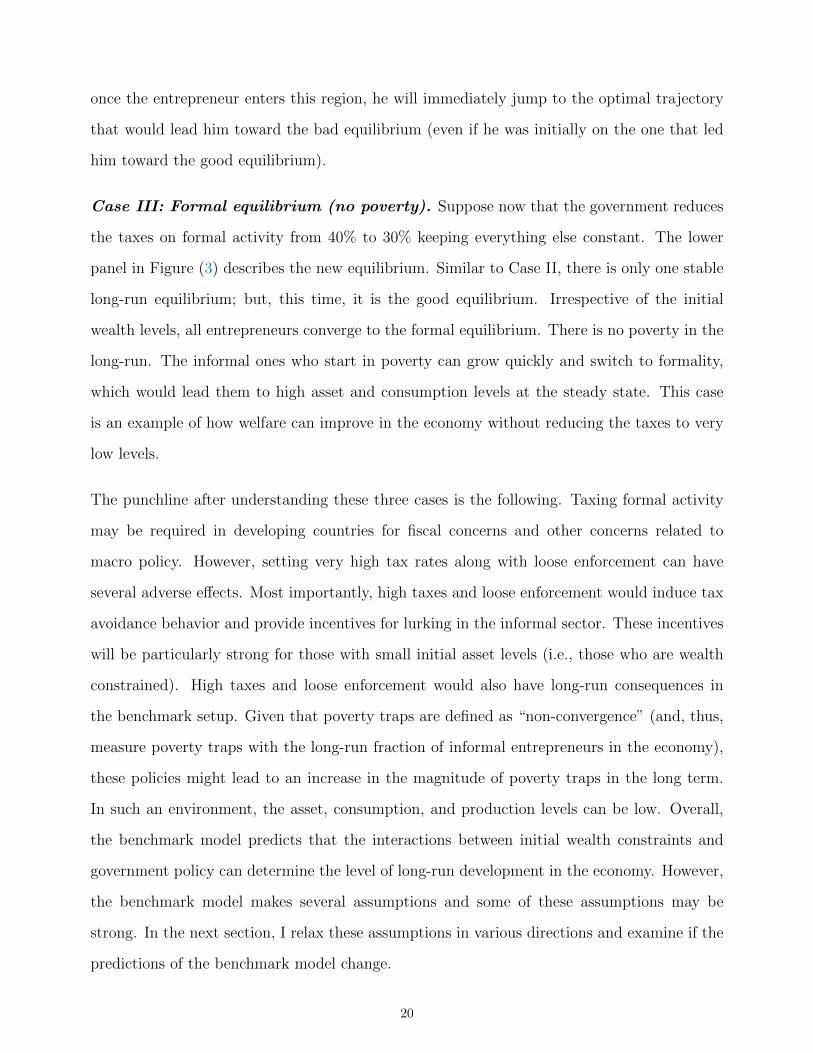
once the entrepreneur enters this region, he will immediately jump to the optimal trajectory

that would lead him toward the bad equilibrium (even if he was initially on the one that led

him toward the good equilibrium).

Case III: Formal equilibrium (no poverty). Suppose now that the government reduces

the taxes on formal activity from 40% to 30% keeping everything else constant. The lower

panel in Figure (3) describes the new equilibrium. Similar to Case II, there is only one stable

long-run equilibrium; but, this time, it is the good equilibrium. Irrespective of the initial

wealth levels, all entrepreneurs converge to the formal equilibrium. There is no poverty in the

long-run. The informal ones who start in poverty can grow quickly and switch to formality,

which would lead them to high asset and consumption levels at the steady state. This case

is an example of how welfare can improve in the economy without reducing the taxes to very

low levels.

The punchline after understanding these three cases is the following. Taxing formal activity

may be required in developing countries for fiscal concerns and other concerns related to

macro policy. However, setting very high tax rates along with loose enforcement can have

several adverse effects. Most importantly, high taxes and loose enforcement would induce tax

avoidance behavior and provide incentives for lurking in the informal sector. These incentives

will be particularly strong for those with small initial asset levels (i.e., those who are wealth

constrained). High taxes and loose enforcement would also have long-run consequences in

the benchmark setup. Given that poverty traps are defined as “non-convergence” (and, thus,

measure poverty traps with the long-run fraction of informal entrepreneurs in the economy),

these policies might lead to an increase in the magnitude of poverty traps in the long term.

In such an environment, the asset, consumption, and production levels can be low. Overall,

the benchmark model predicts that the interactions between initial wealth constraints and

government policy can determine the level of long-run development in the economy. However,

the benchmark model makes several assumptions and some of these assumptions may be

strong. In the next section, I relax these assumptions in various directions and examine if the

predictions of the benchmark model change.

20

Before presenting the extensions, it will be useful to discuss the empirical implications of

the theoretical predictions described above. Hsieh and Klenow (2014) provide a detailed

comparison of the business performances in the U.S., India, and Mexico. They document that,

in the U.S., firms of age 40 are, on average, 8 times larger than the firms of age 5 and below. In

Mexico, firms of age 25 are twice as large as the new plants, but there is no difference between

the 25 and 40 year-old firms. In India, they clearly document that old firms are no larger

than the new ones. Moreover, informality is extensive in Mexico and India, while it is almost

zero in the U.S. Informal plants in Mexico and India are much smaller than formal plants.

These figures suggest that there are large cross-country differences in terms of firm-growth

and firm-size patterns. Hsieh and Klenow (2014) also argue that tax and other institutional

differences across countries can explain these patterns. They argue that, in Mexico and India,

taxes are higher and are more stringently imposed on large businesses—since small businesses

are mostly informal. It is also well-known that enforcement is much looser in developing

countries, which allows informal firms to survive. These facts roughly fit the predictions of

the model and jointly suggest that the design of government policy might have an important

role on entrepreneurial activity as well as firm performance.

4 Extensions of the Model

The benchmark model presented in Section 2 produces clear-cut analytical results. But, as

always, clarity comes at a cost; the model is based on several simplifying assumptions making

the transitional dynamics easier to solve. In this section, I relax some of these assumptions

for the purpose of bringing the model closer to reality. Below I argue that, in most cases,

the qualitative nature of the benchmark model’s results remains unchanged upon relaxing the

corresponding assumption.

4.1 Alternative Tax and Enforcement Settings

For simplicity, the benchmark model assumes that the tax and enforcement policies can be

characterized by two parameters: the tax rate on formal activity, τ ∈ [0, 1], and the probability

21

of getting caught, φ ∈ [0, 1]. The formal entrepreneur always pays the tax τ per unit of

output, whereas the informal entrepreneur pays it only if he gets caught—thus, the effective

tax rate under informality is φτ < τ . The tax rate τ collapses various formal tax items

including the corporate income tax, VAT/turnover taxes, public service taxes, and insurances

into a single tax variable. Similarly, the enforcement measure collapses several enforcement

measures including tax police, mobile tax collectors, computerized detection networks, and

additional safety nets into a single enforcement variable. This parsimonious parametrization

allows for a clean baseline analysis of the effect of government policy on the extent of informal

entrepreneurial activity.

The actual tax and enforcement policies, however, are more complicated and implement ad-

ditional measures. In this subsection, I emphasize the role of two additional factors: (1) fines

and/or asset seizures if caught and (2) the effect of asset size on visibility and, therefore,

on the probability of getting caught. These two elements are documented to be crucially

important cost items for informal entrepreneurs in addition to standard tax and enforcement

measures mentioned above. For example, Djankov, Lieberman, Mukherjee, and Nenova (2002)

and OECD (2009) argue—based on evidence from Latin American, Eastern European, and

Turkic countries—that the legal treatment of tax evasion and informal activity by authorities

have two noteworthy consequences on the operation of informal businesses.14 First, informal

entrepreneurs are highly vulnerable to getting caught by authorities, because they might lose

part or all of their assets—in the form of fines and penalties, if they are “located.” Second, the

probability of getting caught goes up with asset size; thus, informal entrepreneurs are forced

to stay small to minimize their visibility to authorities.

Fines in the form of asset seizures. Suppose that the government imposes a fine on

informal entrepreneurs in the form of asset seizures upon getting caught by the authorities.

Let γ ∈ [0, 1] denote the fraction of assets seized when caught. In this case, the informal

entrepreneur pays the effective tax rate of φ(τ + γ). In some sense, this means that the

actual tax paid by the informal entrepreneurs is higher—conditional on being caught—than

14See also Johnson, Kaufmann, and Shleifer (1997), Johnson, Kaufmann, McMillan, and Woodruff (2000), and Schneider andEnste (2000) for additional evidence and discussion.

22

the formal tax rate.15 Imposing the fine slightly alters the sectoral choice problem. The

entrepreneur is indifferent between operating formally and informally if the condition

θaαf

T (1− τ)− s = θaαiT (1− φ(τ + γ)) (4.1)

is satisfied. This suggests that

daTdγ

=−φaαi

T

αfaαf−1T (1− τ)− αiaαi−1

T (1− φ(τ + γ))< 0, (4.2)

which means that the threshold asset level is lower if the fine is increased. In terms of the

phase diagram, this suggests that fines operate as enforcement; that is, imposing higher asset

seizures on informal entrepreneurs when caught makes the transition easier and has a potential

to reduce the magnitude of poverty traps.

Probability of getting caught as a function of the asset size. Suppose now that the

enforcement parameter—i.e., the probability of getting caught—is an increasing function of

the asset size. To be concrete, I assume φ = φΦ(a) with φ ∈ [0, 1], Φ′(a) > 0, Φ(0) = 0, and

Φ(a) = 1, where a is a large, but finite, number. In this formulation, φ captures the actual

level of enforcement in the economy as a scale effect and Φ(a) determines how this enforcement

level is reflected on the entrepreneur as a function of the asset size. This extension captures the

fact that larger businesses are more visible to authorities and, therefore, staying informal with

a large asset size is harder given a certain level of enforcement. In this case, the indifference

condition becomes

θaαf

T (1− τ)− s = θaαiT (1− φΦ(aT )τ). (4.3)

Totally differentiating Equation (4.3) with respect to aT and φ yields the condition that

daTdφ

=−Φ(aT )τaαi

T

αfaαf−1T (1− τ) + aαi

T φτΦ′(aT )− αiaαi−1T (1− φΦ(aT )τ)

< 0. (4.4)

15Note that we need the parametric restriction φ(τ + γ) < τ to guarantee that operating in the informal sector is still moreattractive. This restriction can be simplified as γ < τ(1− φ).

23

Clearly, the qualitative result that stricter enforcement reduces the asset threshold and makes

the transition easier also holds in this case. However, there is a nuance; now asset size also has a

role in the relationship between the level of enforcement and the asset threshold. Strengthening

the level of enforcement in the economy decreases the threshold asset level and this decline

further affects daT/dφ through the additional term Φ′(aT ) > 0 in the denominator.16 To be

specific, this term makes it harder to become larger and stay informal; thus, the enforcement

policy is even more effective after this extension.17

When the enforcement parameter is modeled as a function of asset size, it becomes natural

to start thinking about a tax differentiation policy along the size distribution. Since small

businesses are less likely to get caught than the large ones, the government may want to pro-

vide some additional incentives that would let them switch into formality. These advantages

may be in the form of reduced tax rates so that informal entrepreneurs with smaller amount

of assets become more likely to operate formally. In fact, empirical studies show that “ex-

emption threshold” type of policies—i.e., businesses below a certain size/revenue threshold

being exempt from paying taxes—provide a significant incentive for the small businesses to

operate formally. However, these studies also show that such thresholds are an important

impediments to the growth of small businesses as they provide incentives to stay small; thus,

small businesses become overrepresented along the size distribution and the “missing mid-

dle” phenomenon emerges.18 Overall, the evidence suggests that providing tax advantages to

smaller businesses increases formality rates among them, but may generate impediments to

their growth; hence, an important policy trade-off emerges.

Notice that the two extensions discussed above have no effect on the qualitative nature of the

results featured by the benchmark model, although there are several interesting nuances that

might alter the quantitative predictions. It is clear that the predictions of the benchmark

model is quite robust to inclusion of any additional policy measure as long as it mimics the

16Compare the conditions (2.7) and (4.4) to observe this difference more clearly.17Note that this interaction will also have implications on the dynamic problem. The first order conditions will change, but

the nature of the results will remain unaltered.18See, e.g., Besley and Burgess (2004), Guner, Ventura, and Yi (2008), Kleven and Waseem (2013), Krueger (2013), and Hsieh

and Olken (2014).

24

behavior of τ and/or φ.19 Of course one can think of other public policy interventions that may

affect the size of informal sector through other channels—such as the demand side measures

that may shift the consumers’ attention from informal to formal products. Such extensions,

albeit interesting, are out of the scope of this paper.

One important point about the nature of the model’s policy setting is that all types of taxes

are collapsed into the single tax parameter τ and all the rest of the policy measures that affect

the probability of getting caught is described by the parameter φ. These two assumptions are

made for the sake of simplicity and analytical tractability. However, a more complex setting

would naturally include different types of taxes, which would have different distortionary

effects on the equilibrium outcomes. There are also other public policy elements including

general regulation, bureaucracy, property rights, corruption, and public good provision. The

paper abstracts from all these different tax and public policy alternatives. When alternative

distortionary taxes are included, the model would have the capacity to answer questions about

optimal fiscal policy—i.e., the government would choose the optimal tax policy in a Ramsey

setting given the optimizing behavior of entrepreneurs [see, e.g., Chari and Kehoe (1999)].

Similarly, the government would also choose φ to determine the optimal compliance in the

informal sector. Then the problem of non-compliance externalities will kick in and complicate

the model. Although these are interesting questions and extensions, they are left out for the

purpose of focusing on the main transitional forces that the model features.

The model also assumes that there is no borrowing or lending. However, it is well-documented

in the literature that businesses relying on internal financial resources grow much slower than

the ones with access to external finance [Carpenter and Petersen (2002), Angelini and Generale

(2008)]. Having unconstrained access to financial markets is an additional incentive to operate

formally and such a borrowing mechanism is not modeled in the paper. Introducing access to

finance for formal entrepreneurs would enhance the dual mechanism described in the paper

and would provide a more realistic basis for the existence of high-growth transformational

businesses. As a consequence, economies with more developed financial systems will likely

19Notice also that all policy measures may also serve to prevent/reduce future tax evasion, because any cost item also appearsin the dynamic problem as part of the present discounted value of output.

25

have a smaller share of informal businesses at the steady state in comparison to the model

with no borrowing and lending, which suggests that the probability of ending up with the

formal equilibrium (no poverty case) will be much higher in economies with more developed

financial systems.

4.2 Endogenous Labor Demand

One of the key assumptions in the benchmark model is that formal sector is more productive

than the informal sector, i.e., one unit of physical asset produces a greater amount of final

good in the formal sector than in the informal sector. This is an empirically valid idea and

is reflected by the assumption αf > αi. (See Section 2 for a detailed discussion of empirical

validity along with references to relevant work.) The cost structure of the model is such that

formal entrepreneurs pay higher taxes than the informal entrepreneurs; thus, operating in the

formal sector is more costly. As a result, the main tradeoff in the model is between higher costs

versus higher benefits in the formal sector. If costs exceeds benefits, then the entrepreneur

chooses to operate informally.

The main purpose of this subsection is to briefly sketch that the assumption αf > αi can be

relaxed as αf = αi = α without changing the qualitative predictions of the benchmark model.

However, relaxing this assumption requires opening an alternative tradeoff channel for the

entrepreneur. To open this alternative channel, I propose relaxing another assumption in the

model: the assumption that labor input is fixed—i.e., it is set to 1—in the production function

of the entrepreneur. In this alternative setup, the entrepreneur is, by definition, small, it takes

the wage rate as given, and chooses how much labor to hire at each time period. Assume that

formal and informal entrepreneurs pay the same wage per unit of work to their employees.

This setup necessitates invoking the assumption that probability of getting caught goes up

with the asset size. This will be the new tradeoff channel. The intuition is as follows. The

production process is homogeneous across sectors.

The informal entrepreneur chooses to use less capital and more labor—because greater capital

stock is easier to detect and capital can but labor cannot be seized when caught. The formal

26

entrepreneur, on the other hand, can use more physical assets and less labor. Now the sectoral

choice depends on the following tradeoff: (i) whether to hire an additional worker and keep

the asset size small to minimize the probability of getting caught in exchange for paying lower

taxes, (ii) or to expand the business by accumulating greater assets to enjoy greater profits

without worrying about higher taxes paid in the formal sector. Similar to the benchmark

model, the threshold will depend on the tax and enforcement policies and the initial asset

levels will determine who will converge to which equilibrium. The punchline is that it is

possible to relax the assumption αf > αi in sensible ways without altering the predictions of

the benchmark model.

4.3 Uncertainty

It is possible to incorporate into the model aggregate and/or idiosyncratic uncertainty af-

fecting the entrepreneur’s decisions. The standard framework to think of such an extension

is to make θ stochastic—simply via a Markovian transition matrix—to capture the cyclical

nature of physical capital investments. Using a version of the canonical investment under

uncertainty framework with adjustment costs [see Lucas and Prescott (1971)], one can show

that uncertainty affects the entrepreneur’s expectations on future returns to physical assets.

The stationary character of the standard shock structures will let the equilibrium solution

to settle down “on average” to a long-run equilibrium or multiple equilibria. Different from

the benchmark model, these equilibria depend not only on the government policies and initial

wealth positions, but on the distribution of shocks and the structure of adjustment costs. The

simulations of this stochastic model will demonstrate the additional result that the threshold

variable is counter-cyclical—i.e., it declines (goes up) in good (bad) times making it easier

(harder) to transition from informal to formal sector and reducing (magnifying) the size of

poverty traps.

Another possibility is to also incorporate a fixed cost of transition to formal sector. This

fixed costs might reflect the costs of tax registration and formal business start-ups. When a

combination of uncertainty and fixed costs is in effect, there will be lumpiness in the decision

27

to switch from informality to formality, as the entrepreneur will develop an optimal strategy

reflecting a Ss type of behavior.20 To be specific, there will be a period of “inaction” in which

the informal entrepreneur will stay on the asset threshold without switching to formality.

When the positive shocks accumulate high enough positive returns that overcome the fixed

costs, the informal entrepreneur will switch to formality. This time “the switching time to

formality” will depend on government policy as well as the other variables mentioned above.

In all these extensions, the qualitative feature of the results will resemble the results pro-

duced by the benchmark model. Of course, these models will bring additional insights such

as predictions regarding the cyclical nature of poverty traps as well as the state-dependent

effect of government policy on entrepreneurial decisions. Moreover, these extensions will help

incorporating other policy measures into the model such as capital losses in case of negative

shocks and associated loss deductibility policies. Such policies will smooth out the negative

impacts of bad shocks and limit the increase in the size of poverty traps in recessions. How-

ever, I believe that the costs of mathematical complexity brought in by these extensions will

exceed their returns. In particular, it will not be possible to present an analytically tractable

transitional dynamics similar to the one presented in Figure (1). Therefore, for the purpose

of keeping the model compact and analytically tractable, I ignore presenting the full solution

of the stochastic model.

4.4 Redistribution

The benchmark model implicitly assumes that government spending is wasteful; that is, the

tax revenues collected are not rebated back to the entrepreneurs and, instead, they are spent

for some unproductive purpose, i.e., wasted. In this subsection, I relax this assumption by

explicitly incorporating a government budget constraint and a simple redistribution scheme

into the model.

The benchmark model is basically a microeconomic model—since it describes the behavior

of an individual entrepreneur—and aggregation has never been a concern. This simple setup

20See Stokey (2008) for an excellent review of the models embodying Ss type of behavior.

28

facilitates studying both the steady state and transitional dynamics implications of hetero-

geneity in the initial asset levels on the main predictions of the model. In a model with a formal

redistribution of tax revenues, heterogeneity will enormously limit the analytical tractability

of the model since it will be a must to follow what happens to the distribution of assets across

entrepreneurs over time. In particular, the threshold asset level aT—the threshold determining

the entrepreneur’s sectoral choice—will be time-dependent and individual-specific, which will

make the transitional dynamics very hard to characterize. In what follows, I will start with

the steady state implications of redistribution and then I will sketch out the dynamic elements

of the problem as fully as possible.

Suppose that at the steady state, the entrepreneur chooses whether to operate formally versus

informally. Different from the benchmark model, the formal entrepreneur receives a lump-sum

transfer Lss, where the subscript denotes steady state, and the informal entrepreneur does not.

The sectoral choice margin is now determined by the equation

θaαf

T,ss(1− τ)− s+ Lss = θaαiT,ss(1− φτ). (4.5)

Totally differentiating the threshold level aT with respect to Lss gives

daT,ssdLss

=−1

αfθaαf−1T,ss (1− τ)− αiθaαi−1

T,ss (1− φτ)< 0, (4.6)

which suggests that introducing redistribution makes the transition from informality to for-

mality easier by reducing the threshold asset level. The main finding of the benchmark model

was that the government could reduce poverty traps by reducing taxes on formal activity and

strengthening enforcement to prevent informality. The result featured in expression (4.6),

by itself, suggests that the government can intervene poverty traps via a third channel: re-

distribution. An appropriately designed redistribution scheme can provide incentives for less

wealth-constrained entrepreneurs to invest more intensively in their businesses and switch to

formality.

To sketch off-the-steady-state dynamics, one has to write down the government budget con-

29

straint explicitly. Each period, the government collects the tax revenues and redistributes

them equally across the formal entrepreneurs in the form of lump-sum transfers L(t). Let

G(t)—a cumulative distribution function with finite domain—denote the overall asset distri-

bution in the economy. At each time period, there exists a threshold asset level aT (t) above

which the entrepreneurs operate in the formal sector and below which they operate in the

informal sector. The government budget constraint can now be written as

φτ

∫ aT (t)

0

a(t)dG(t) + τ

∫ ∞aT (t)

a(t)d[1−G(t)] =

∫ ∞aT (t)

L(t)d[1−G(t)]. (4.7)

In words, the formal entrepreneur pays the tax and the informal entrepreneur pays only if he

gets caught.21 The aggregate tax revenues are redistributed back to the formal entrepreneurs

only. The complexity here is that we start from a given initial asset distribution G(0) and

the economy moves from here to a stationary steady state asset distribution Gss. Since L(t)

is time dependent in this setup, aT (t) is also time dependent. How aT (t) evolves, in turn,

determines how G(t) evolves. Under standard functional form assumptions stated in Lucas

and Moll (2014) and invoking convergence rules, the law of motion for G(t) can be formulated

explicitly and it can be shown to converge to a steady state asset distribution Gss, for which

aT,ss and Lss are constant numbers. In particular, the condition

limt→∞

aT (t) = 0 (4.8)

must hold to guarantee convergence to a steady-state solution.

It is clear in this exercise that switching from wasteful government spending from a lump-sum

redistribution scheme provides incentives to become a formal entrepreneur by reducing the

threshold asset level. What is not so clear is the effect of a change in government policy under

redistribution. The next point to mention, therefore, is related to the effectiveness of tax and

enforcement policy changes under the redistribution regime. Suppose that the tax rate on

formal activity is reduced. Reduced taxes will provide an incentive to switch to formality, as

21This can be interpreted as follows: each period a φ fraction of informal entrepreneurs are caught and the correspondingamount φτ per unit of output is added on the total tax revenue.

30

in the benchmark model. However, there might be a competing negative force in the presence

of redistribution: if the decline in taxes reduce the tax revenues, then, depending on the

elasticities and asset distribution, this may lead to a decline in the lump-sum transfer L and,

thus, may provide an indirect disincentive for formality. The net effect of the tax reduction

will depend on the relative strengths of these two forces.

An important point to mention is that the functional form of the asset distribution G may

affect the extent of these incentives. It is well-documented in the empirical literature that

the size distribution of firms is of the Pareto form.22 This Pareto form will increase the

effectiveness of the redistribution policy, because tax revenues collected from the large firms

on the right tail will be less likely to deter formal economic activity; these revenues, in turn,

may generate a greater incentive for the small atomistic informal entrepreneurs to switch to

formality.

To conclude; an appropriately designed redistribution system will provide incentives for in-

formal entrepreneurs to switch to formality. However, different from the benchmark model,

the effectiveness of tax and enforcement policies are more ambiguous under a redistribution

scheme; since, the direct effect of a change in tax (or enforcement) policy might be negated

by the indirect effect coming from the change in the redistributed amount.

5 Concluding Remarks

There is a large shadow economy literature mainly arguing that the share of the informal

activity is a function of the tax and enforcement policies. The main idea in this literature is

that high taxes on formal production and loose enforcement, which is often the case in LDCs,

encourage informal economic activity. My starting point also rests on this idea; that is, I start

with a model in which entrepreneurs choose whether to operate in the formal versus informal

sectors. The sectoral choice problem is a function of tax and enforcement policies, consistent

with the literature.

22See, for example, Simon and Bonini (1958), Ijiri and Simon (1964), Axtell (2001), and Luttmer (2007).

31

The novelty that this paper introduces is the idea that the interaction between wealth con-

straints and government policy jointly determines the fraction of entrepreneurs entrapped

in the informal economy forever. When taxes are high and enforcement is loose, initially

constrained entrepreneurs choose to operate informally, they have no incentives to make ex-

pansionary investments in their businesses because formal activity is costly, and, as a result,

they stay small and operate informally in the long run. This is literally a poverty trap. The

main insight in this paper is that poverty traps are related to government policy and, therefore,

can be reduced in magnitude. To be precise, I show that lowering taxes over formal produc-

tion and tightening enforcement will reduce the magnitude of poverty traps and encourage

entrepreneurs to become large businesses operating in the formal economy in the long run.

This paper is also related to the literature studying the link between wealth constraints and en-

trepreneurship. That entrepreneurs are constrained by their initial wealth levels is a common

finding in the literature. I show that, given an initial wealth level, whether an entrepreneur can

transition into formal economy or trapped in the informal economy depends on government

policy; that is, government policy is the mediating force determining whether initially con-

strained informal entrepreneurs can expand their businesses and turn into formal enterprises

or not. The main policy implication of these results is that governments should decrease taxes

on formal production and increase enforcement levels, if they want to combat informality and

reduce the magnitude of poverty traps.

I also show that introducing an appropriately designed redistribution system may serve as a

third policy mechanism—besides reducing taxes and strengthening enforcement—to encourage

formal entrepreneurship. One caveat, however, is that the effect of tax and enforcement

policies on informality becomes more ambiguous when they are implemented under a lump-

sum redistribution system. There will be a direct effect of a tax cut on providing incentives

for formal production, just as in the benchmark model. There will also be an indirect effect

of the tax cut on the redistributed amount. If the amount of the lump-sum transfer goes

down as a response to the tax cut, then the sign of this indirect effect will depend on the

relevant elasticities and the overall distribution of assets in the economy. This ambiguity calls

32

for additional research about the effect of government policy on informal economic activity

when a redistribution scheme is in effect.

33

References

Amaral, P. and E. Quintin (2006): “A Competitive Model of the Informal Sector,”

Journal of Monetary Economics, 53, 1541–1553.

Angelini, P. and A. Generale (2008): “On the Evolution of Firm Size Distributions,”

American Economic Review, 98, 426–438.

Axtell, R. L. (2001): “Zipf Distribution of U.S. Firm Sizes,” Science, 293, 1818–1820.

Ayyagari, M., T. Beck, and A. Demirguc-Kunt (2007): “Small and Medium Enter-

prises across the Globe,” Small Business Economics, 29, 415–434.

Azariadis, C. (1996): “The Economics of Poverty Traps Part One: Complete Markets,”

Journal of Economic Growth, 1, 449–486.

Banerjee, A. V. (2004): “Contracting Constraints, Credit Markets and Economic Devel-

opment,” in Advances in Economics and Econometrics: Theory and Applications, ed. by

M. Dewatripont, L. P. Hansen, and S. J. Turnovsky, Cambridge, UK: Cambridge University

Press, vol. III, chap. 1, 1–46.

Banerjee, A. V. and A. F. Newman (1993): “Occupational Choice and the Process of

Development,” Journal of Political Economy, 101, 274–298.

Benabou, R. J. (1993): “Workings of a City: Location, Education, and Production,” Quar-

terly Journal of Economics, 108, 619–652.

Besley, T. J. and R. Burgess (2004): “Can Labor Regulations Hinder Economic Perfor-

mance? Evidence from India,” Quarterly Journal of Economics, 119, 91–134.

Blanchflower, D. and A. J. Oswald (1998): “What Makes An Entrepreneur?” Journal

of Labor Economics, 16, 26–60.

Boadway, R., M. Marchand, and P. Pestieau (1991): “Optimal Linear Income Taxa-

tion in Models with Occupational Choice,” Journal of Public Economics, 46, 133–162.

34

Buera, F. J. (2008): “Persistency of Poverty, Financial Frictions, and Entrepreneurship,”

Unpublished manuscript, Northwestern University.

Cagetti, M. and M. De Nardi (2009): “Estate Taxation, Entrepreneurship, and Wealth,”

American Economic Review, 99, 85–111.

Carpenter, R. E. and B. C. Petersen (2002): “Is the Growth of Small Firms Con-

strained by Internal Finance?” Review of Economics and Statistics, 84, 298–309.

Chari, V. V. and P. J. Kehoe (1999): “Optimal Fiscal and Monetary Policy,” in Handbook

of Macroeconomics, ed. by K. J. Arrow and M. D. Intriligator, Elsevier, vol. 1, chap. 26,

1671–1745.

Cooper, R. W. and J. C. Haltiwanger (2006): “On the Nature of Capital Adjustment

Costs,” Review of Economic Studies, 73, 611–633.

Cullen, J. B. and R. H. Gordon (2007): “Taxes and Entrepreneurial Risk-Taking: The-

ory and Evidence for the U.S.” Journal of Public Economics, 91, 1479–1505.

de Meza, D. (2002): “Overlending?” Economic Journal, 117, F17–F31.

de Meza, D. and C. Southey (1996): “The Borrower’s Curse: Optimism, Finance, and

Entrepreneurship,” Economic Journal, 106, 375–386.

De Paula, A. and J. A. Scheinkman (2011): “The Informal Sector: An Equilibrium

Model and Some Empirical Evidence from Brazil,” Review of Income and Wealth, 57, S8–

S26.

De Soto, H. (1989): The Other Path: The Invisible Revolution in the Third World, New

York, NY: Harper and Row.

——— (2000): The Mystery of Capital: Why Capitalism Triumphs in the West and Fails

Everywhere Else, New York, NY: Basic Books.

Decker, R., J. C. Haltiwanger, R. Jarmin, and J. Miranda (2014): “The Role

of Entrepreneurship in US Job Creation and Economic Dynamism,” Journal of Economic

Perspectives, 28, 3–24.

35

Djankov, S., I. Lieberman, J. Mukherjee, and T. Nenova (2002): “Going Informal:

Benefits and Costs,” Unpublished manuscript, World Bank.

Durlauf, S. N. (1993): “Nonergodic Economic Growth,” Review of Economic Studies, 60,

349–366.

——— (1996): “A Theory of Persistent Income Inequality,” Journal of Economic Growth, 1,

75–93.

Evans, D. S. and B. Jovanovic (1989): “An Estimated Model of Entrepreneurial Choice

under Liquidity Constraints,” Journal of Political Economy, 97, 808–827.

Farrell, D. (2004): “The Hidden Dangers of the Informal Economy,” McKinsey Quarterly,

3, 26–37.

Fossen, F. M. and D. Rostam-Afschar (2012): “Precautionary and Entrepreneurial Sav-

ings: New Evidence from German Households,” Oxford Bulletin of Economics and Statistics,

75, 528–555.

Friedman, E., S. Johnson, D. Kaufmann, D., and P. Zoido-Lobaton (2000): “Dodg-

ing the Grabbing Hand: The Determinants of Unofficial Activity in 69 Countries,” Journal

of Public Economics, 76, 459–493.

Galor, O. and H. E. Ryder (1989): “Existence, Uniqueness, and Stability of Equilib-

rium in an Overlapping-Generations Model with Productive Capital,” Journal of Economic

Theory, 49, 360–375.

Galor, O. and J. Zeira (1993): “Income Distribution and Macroeconomics,” Review of

Economic Studies, 60, 35–52.

Gentry, W. M. and R. G. Hubbard (2004): “Entrepreneurship and Household Saving,”

The B.E. Journal of Economic Analysis & Policy, 4, 1–55.

Gordon, R. H. (1998): “Can High Personal Tax Rates Encourage Entrepreneurial Activity?”

IMF Staff Papers, 45, 49–80.

36

Guner, N., G. Ventura, and X. Yi (2008): “Macroeconomic Implications of Size-

Dependent Policies,” Review of Economic Dynamics, 11, 721–744.

Haltiwanger, J. C. (2012): “Job Creation and Firm Dynamics in the U.S.” in Innovation

Policy and the Economy, ed. by J. Lerner and S. Stern, University of Chicago Press, NBER

Book Series, 17–38.

Haltiwanger, J. C., R. Jarmin, and J. Miranda (2013): “Who Creates Jobs? Small

vs Large vs Young,” Review of Economics and Statistics, 95, 347–361.

Holtz-Eakin, D., D. Joulfaian, and H. S. Rosen (1994): “Sticking It Out: En-

trepreneurial Survival and Liquidity Constraints,” Journal of Political Economy, 102, 53–75.

Hsieh, C.-T. and P. J. Klenow (2014): “The Life Cycle of Plants in India and Mexico,”

Quarterly Journal of Economics, 129, 1035–1084.

Hsieh, C.-T. and B. A. Olken (2014): “The Missing “Missing Middle”,” Journal of

Economic Perspectives, 28, 89–108.

Hubbard, G. and W. M. Gentry (2000): “Tax Policy and Entrepreneurial Entry,” Amer-

ican Economic Review, 90, 283–287.

——— (2005): “‘Success Taxes,’ Entrepreneurial Entry, and Innovation,” in Innovation Policy

and the Economy, ed. by A. B. Jaffe, J. Lerner, and S. Stern, MIT Press, vol. 5, 87–108.

Hurst, E. and A. Lusardi (2004): “Liquidity Constraints, Household Wealth, and En-

trepreneurship,” Journal of Political Economy, 112, 319–347.

Ihrig, J. and K. S. Moe (2004): “Lurking in the Shadows: The Informal Sector and

Government Policy,” Journal of Development Economics, 73, 541–557.

Ijiri, Y. and H. A. Simon (1964): “Business Firm Growth and Size,” American Economic

Review, 54, 77–89.

IMF (2016): “Acting Now, Acting Together,” .

37

Johnson, S., D. Kaufmann, J. McMillan, and C. Woodruff (2000): “Why Do Firms

Hide? Bribes and Unofficial Activity After Communism,” Journal of Public Economics, 76,

495–520.

Johnson, S., D. Kaufmann, and A. Shleifer (1997): “The Unofficial Economy in Tran-

sition,” Brookings Papers on Economic Activity, 28, 159–240.

Johnson, S., D. Kaufmann, and P. Zoido-Lobaton (1998): “Regulatory Discretion and

the Unofficial Economy,” American Economic Review Papers & Proceedings, 88, 387–392.

Jones, C. I. (2008): “Comment on La Porta and Shleifer “The Unofficial Economy and

Economic Development”,” Brookings Papers on Economic Activity, 39, 353–359.

Kanbur, S. M. (1981): “Risk Taking and Taxation: An Alternative Perspective,” Journal

of Public Economics, 15, 163–184.

Kerr, W. R. and R. Nanda (2011): “Financing Constraints and Entrepreneurship,” in

Handbook of Research on Innovation and Entrepreneurship, ed. by D. Audretsch, O. Falck,

and S. Heblich, Cheltenham, UK: Edward Elgar Publishing, 88–103.

Kleven, H. J. and M. Waseem (2013): “Using Notches to Uncover Optimization Frictions

and Structural Elasticities: Theory and Evidence from Pakistan,” Quarterly Journal of

Economics, 128, 669–723.

Krueger, A. O. (2013): “The Missing Middle,” in Economic Reform in India: Challenges,

Prospects, and Lessons, ed. by N. C. Hope, A. Kochar, R. Noll, and T. N. Srinivasan,

Cambridge University Press, chap. 9.

La Porta, R. and A. Shleifer (2008): “The Unofficial Economy and Economic Develop-

ment,” Brookings Papers on Economic Activity, 39, 275–363.

——— (2014): “Informality and Development,” Journal of Economic Perspectives, 28, 109–

126.

Li, W. (2002): “Entrepreneurship and Government Subsidies: A General Equilibrium Anal-

ysis,” Journal of Economic Dynamics and Control, 26, 1815–1844.

38

Lindh, T. and H. Ohlsson (1998): “Self-Employment and Wealth Inequality,” Review of

Income and Wealth, 44, 25–42.

Loayza, N. V. (1996): “The Economics of the Informal Sector: A Simple Model and Some

Empirical Evidence from Latin America,” Carnegie Rochester Conference Series on Public

Policy, 45, 129–162.

Lucas, R. E. J. and B. Moll (2014): “Knowledge Growth and the Allocation of Time,”

Journal of Political Economy, 122, 1–51.

Lucas, R. E. J. and E. C. Prescott (1971): “Investment Under Uncertainty,” Econo-

metrica, 39, 659–681.

Luttmer, E. G. J. (2007): “Selection, Growth, and the Size Distribution of Firms,” Quar-

terly Journal of Economics, 122, 1103–1144.

McKenzie, D. J. and C. Woodruff (2006): “Do Entry Costs Provide an Empirical Basis

for Poverty Traps? Evidence from Mexican Microenterprises,” Economic Development and

Cultural Change, 55, 3–42.

McKinsey (1998): “Productivity – The Key to An Accelerated Development Path in Brazil,”

McKinsey Global Institute Country Report.

Mookherjee, D. and D. Raj (2002): “Contractual Structure and Wealth Accumulation,”

American Economic Review, 92, 818–849.

Murphy, K. M., A. Shleifer, and R. W. Vishny (1989): “Income Distribution, Market

Size, and Industrialization,” Quarterly Journal of Economics, 104, 537–564.

Nanda, R. (2010): “Entrepreneurship and the Discipline of External Finance,” Unpublished

manuscript, Harvard University.

OECD (2009): “Competition Policy and the Informal Economy,” Policy Roundtable.

Peck, R. M. (1989): “Taxation, Risk, and Returns to Scale,” Journal of Public Economics,

40, 319–330.

39

Quadrini, V. (2000): “Entrepreneurship, Saving, and Social Mobility,” Review of Economic

Dynamics, 3, 1–40.

Rauch, J. E. (1991): “Modeling the Informal Sector Formally,” Journal of Development

Economics, 35, 33–48.

Schneider, F., A. Buehn, and C. E. Montenegro (2010): “New Estimates for the

Shadow Economies all over the World,” International Economic Journal, 24, 443–461.

Schneider, F. G. and D. H. Enste (2000): “Shadow Economies: Size, Causes, and

Consequences,” Journal of Economic Literature, 38, 77–114.

Schoar, A. (2010): “The Divide between Subsistence and Transformational Entrepreneur-

ship,” in Innovation Policy and the Economy, ed. by J. Lerner and S. Stern, University of

Chicago Press, vol. 10 of NBER Book Series, 57–81.

Simon, H. A. and C. P. Bonini (1958): “The Size Distribution of Business Firms,” Amer-

ican Economic Review, 48, 607–617.

Stokey, N. L. (2008): The Economics of Inaction: Stochastic Control Models with Fixed

Costs, Princeton, NJ: Princeton University Press.

Thomas, J. J. (1992): Informal Economic Activity, Ann Arbor, MI: University of Michigan

Press.

Tumen, S. (2016): “Informality as a Stepping Stone: A Search-Theoretical Assessment of

Informal Sector and Government Policy,” Central Bank Review, 16, 109–117.

WorldBank (2005): “Investment Climate Assessment: Brazil,” Country Background Re-

port.

40

0 2 4 6 8 10 12 14 16 18 20−0.2

−0.1

0

0.1

0.2

0.3

0.4

0.5

0.6

0.7

0.8

Physical Assets

Con

sum

ptio

n

aT

afssaiss

0 2 4 6 8 10 12 14 16 18 20−0.2

0

0.2

0.4

0.6

0.8

1

1.2

1.4

Physical Assets

Con

sum

ptio

n

aT

aiss afss

Figure 3: Cases for unique long-run equilibrium. I use the same parameter configuration as the oneproposed in Figure (2). The difference is that the tax rate is no more 0.4; it is increased to 0.5 on the upperpanel and decreased to 0.3 on the lower panel.

41