Entanglement Propagation

Moshe Rozali

University of British Columbia

Quantum Matter, Spacetime and InformationYITP Kyoto, June 2016

Based on:

M.R., Mukund Rangamani, Alexandre Vincart-Emard (arXiv:1512.03478,JHEP) + work in progress together with Anson Wong.

Moshe Rozali (UBC) Quantum Matter, Spacetime and Information YITP Kyoto, June 2016 1 / 12

Outline:

1 Introduction and Motivation

2 Setup: Local QuenchesQuenchingHydrodynamical Evolution

3 Entanglement PropagationInformation LightconeInformation VelocityEntanglement Decay

4 Future Directions

Moshe Rozali (UBC) Quantum Matter, Spacetime and Information YITP Kyoto, June 2016 2 / 12

Introduction and Motivation

Introduction and Motivation

Non-equilibrium many-body systems are interesting, gauge-gravityduality is one way to make general statements, in non-integrablesystems.

Entanglement entropy is an interesting quantity, quantifying thedistribution of information in a quantum state.

In holography, EE is easy to calculate using the RT, or more generallythe HRT prescription.

It is interesting to see the behaviour of the entanglement innon-equilibrium situation, where it goes one step further beyond localprobes of the system. For example it is interesting to probethermalization using the EE.

Directly related (holographically and otherwise) to other measures of”scrambling” of quantum information.

Moshe Rozali (UBC) Quantum Matter, Spacetime and Information YITP Kyoto, June 2016 3 / 12

Introduction and Motivation

Introduction and Motivation

Much attention was given to entanglement growth following a globalquench, resulting in a beautiful picture of ”entanglement tsunami”,quantified in terms of tsunami velocity vT which expresses the rate ofgrowth of EE following the quench.

We are interested in entanglement spread, i.e the spatial propagationof EE following a localized excitation of the system.

This is a spatially resolved version of the same experiment: start thesystem in an atypical, locally excited state, see how the entanglementon different scales returns to the equilibrium value.

Some previous attacks on this problem involved taking certain limits(e.g. shock waves), or working in 1+1 dimensions. We will use anexact numerical solution of the bulk equations to access the exactresults for a generic point in parameter space.

Moshe Rozali (UBC) Quantum Matter, Spacetime and Information YITP Kyoto, June 2016 4 / 12

Setup: Local Quenches Quenching

Quenching

We study a 2+1 dimensional strongly coupled CFT, dual to 3+1dimensional asymptotically AdS4 spacetime. Starting with a thermalstates of temperature T , dual to a bulk black brane, we source the metricby turning on a pulse of scalar field, dual to a relevant operator in theboundary CFT.

We choose the source function to be φ0(t, x) = f (x)g(t) with

f (x) =α

2

[tanh

(x + σ

4s

)− tanh

(x − σ

4s

)], g(t) = sech2

(t − tq∆

tq

).

With it, we can ramp up the scalar field to reach its maximum value α attime t = tq∆ before it drops and vanishes again. The parameters{s, tq,∆} are chosen to facilitate the numerics, whereas σ determines thespatial width of the perturbation and α is the amplitude.

Moshe Rozali (UBC) Quantum Matter, Spacetime and Information YITP Kyoto, June 2016 5 / 12

Setup: Local Quenches Hydrodynamical Evolution

Hydrodynamical Evolution

Soon after the injection of the localized pulse of energy the evolution ofthe energy-momentum tensor is described by hydrodynamics, because offast (local) thermalization typical of holographic theories.

Since our perturbation excites the sound mode of the system, we have theinitial energy-momentum perturbation dispersing at the speed of sound.Below we see a typical profile of the energy density as function of (x,t)

Curiously, the initial perturbation splits to two localized perturbations aftersome time; those follow the expected hydrodynamic evolution.

Moshe Rozali (UBC) Quantum Matter, Spacetime and Information YITP Kyoto, June 2016 6 / 12

Entanglement Propagation

Evolution of the EE

In the situation described above, we look at the EE on different scales. Wechoose to look at boundary strips

A = {(x , y) | x ∈ (−L, L), y ∈ R} , ∂A = {(x , y) | x = ±L, y ∈ R}

We track the entanglement (quantified as the difference from theentanglement in the unquenched thermal state), for strips centred aroundthe location of the quench. This result in the function ∆SA(L, t),depending on the size of the entangling surface and time.

We have 3 dimensionful parameters or equivalently 2 dimensionless ones.

Temperature, or equivalently energy density.

Quench amplitude α.

Quench width σ.

The temperature T determine the range of sizes L which we can probeusing our methods. Since we do not access the region behind the horizon,it follows that L & T . This is sufficient to find some universal results.

Moshe Rozali (UBC) Quantum Matter, Spacetime and Information YITP Kyoto, June 2016 7 / 12

Entanglement Propagation

Evolution of the EE

In the situation described above, we look at the EE on different scales. Wechoose to look at boundary strips

A = {(x , y) | x ∈ (−L, L), y ∈ R} , ∂A = {(x , y) | x = ±L, y ∈ R}

We track the entanglement (quantified as the difference from theentanglement in the unquenched thermal state), for strips centred aroundthe location of the quench. This result in the function ∆SA(L, t),depending on the size of the entangling surface and time.

We have 3 dimensionful parameters or equivalently 2 dimensionless ones.

Temperature, or equivalently energy density.

Quench amplitude α.

Quench width σ.

The temperature T determine the range of sizes L which we can probeusing our methods. Since we do not access the region behind the horizon,it follows that L & T . This is sufficient to find some universal results.

Moshe Rozali (UBC) Quantum Matter, Spacetime and Information YITP Kyoto, June 2016 7 / 12

Entanglement Propagation

Evolution of the EE

In the situation described above, we look at the EE on different scales. Wechoose to look at boundary strips

A = {(x , y) | x ∈ (−L, L), y ∈ R} , ∂A = {(x , y) | x = ±L, y ∈ R}

We track the entanglement (quantified as the difference from theentanglement in the unquenched thermal state), for strips centred aroundthe location of the quench. This result in the function ∆SA(L, t),depending on the size of the entangling surface and time.

We have 3 dimensionful parameters or equivalently 2 dimensionless ones.

Temperature, or equivalently energy density.

Quench amplitude α.

Quench width σ.

The temperature T determine the range of sizes L which we can probeusing our methods. Since we do not access the region behind the horizon,it follows that L & T . This is sufficient to find some universal results.

Moshe Rozali (UBC) Quantum Matter, Spacetime and Information YITP Kyoto, June 2016 7 / 12

Entanglement Propagation Information Lightcone

Information Lightcone

Our main result: For (nearly) all choices of parameters we find linear(ballistic) growth of ∆SA(L, t). We quantify that by looking at

Lpeak(t) = ArgMaxL ∆SA(L, t)

Note that unlike various limits taken previously, the maximum itselfMaxL∆SA(L, t) is not constant.

Note that for L > σ there is some time delay for which ∆SA(L, t) exactlyvanishes, by bulk causality. By linear dispersion we mean then that afterthat time t0:

Lpeak(t) = vE ∗ t + constant

Moshe Rozali (UBC) Quantum Matter, Spacetime and Information YITP Kyoto, June 2016 8 / 12

Entanglement Propagation Information Lightcone

Information Lightcone

Our main result: For (nearly) all choices of parameters we find linear(ballistic) growth of ∆SA(L, t). We quantify that by looking at

Lpeak(t) = ArgMaxL ∆SA(L, t)

Note that unlike various limits taken previously, the maximum itselfMaxL∆SA(L, t) is not constant.

Note that for L > σ there is some time delay for which ∆SA(L, t) exactlyvanishes, by bulk causality. By linear dispersion we mean then that afterthat time t0:

Lpeak(t) = vE ∗ t + constant

Moshe Rozali (UBC) Quantum Matter, Spacetime and Information YITP Kyoto, June 2016 8 / 12

Entanglement Propagation Information Velocity

Information Velocity

The information lightcone is analogous to the Lieb-Robinson velocity inspin systems. Like the LR velocity we find that vE is state-dependent, i.e.depends on parameters of the quench.

Note that vE is a priori different from other entanglement speeds (e.g. thetsunami velocity of Liu and Suh which has to do with entanglementgrowth rate).

We find lower and upper bounds for the information velocity, and someuniversal results in certain limits.

Moshe Rozali (UBC) Quantum Matter, Spacetime and Information YITP Kyoto, June 2016 9 / 12

Entanglement Propagation Information Velocity

Information Velocity

There is an interesting interplay between the size of the entangling surfaceL and the width of the pulse σ:

When L < σ the quench looks like a global one. When we furthertake sufficiently high T , we find that vE = 1, regardless of theamplitude of quench (including values well within the non-linearregime). The speed of light is a bound for all cases, and the bound issaturated in this regime.

When we increase L past σ, we enter a different linear regime with adifferent velocity. The change in slope when L ∼ σ is abrupt.

When the quench is in the linear response regime, and for surfacessuch that L > σ, we find that our information velocity is numericallyvery close to the tsunami velocity. However, increasing the amplitudeof the quench increases the information velocity as well. The tsunamivelocity is a lower bound for the parameter range we probe.

Moshe Rozali (UBC) Quantum Matter, Spacetime and Information YITP Kyoto, June 2016 10 / 12

Entanglement Propagation Entanglement Decay

Entanglement Decay

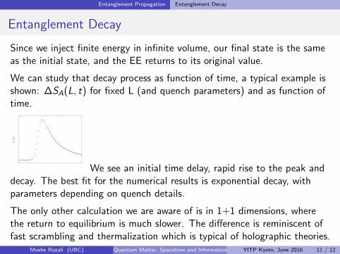
Since we inject finite energy in infinite volume, our final state is the sameas the initial state, and the EE returns to its original value.

We can study that decay process as function of time, a typical example isshown: ∆SA(L, t) for fixed L (and quench parameters) and as function oftime.

0 2 4 6 8

0.0

0.1

0.2

0.3

0.4

0.5

0.6

t

DS

AHtL

We see an initial time delay, rapid rise to the peak anddecay. The best fit for the numerical results is exponential decay, withparameters depending on quench details.

The only other calculation we are aware of is in 1+1 dimensions, wherethe return to equilibrium is much slower. The difference is reminiscent offast scrambling and thermalization which is typical of holographic theories.

Moshe Rozali (UBC) Quantum Matter, Spacetime and Information YITP Kyoto, June 2016 11 / 12

Future Directions

Future Directions

In order of ambition:

It would be nice to have a qualitative model reproducing some of thenumerical results, making connection to other non-integrable models.

Extension to other theories and states , e.g. massive theories andfinite density black holes, especially in the extremal limit (inprogress).

Quench and annealing past critical points. In particular mutualinformation should be more sensitive to phase structure.

Relation to other manifestations of information and scrambling:tsunami velocity, butterfly velocity and shock waves, Lieb-Robinsonvelocity.

More generally: why does entanglement transport so simply. How isthat related to microscopic chaos, and to other forms of transport?

Moshe Rozali (UBC) Quantum Matter, Spacetime and Information YITP Kyoto, June 2016 12 / 12