Ensemble Optimization Techniques for Classical and Quantum Systems
50
Ensemble Optimization Techniques for Classical and Quantum Systems S. Trebst 1 and M. Troyer 2 1 Microsoft Research and Kavli Institute for Theoretical Physics, University of California, Santa Barbara, CA 93106, USA [email protected] 2 Theoretische Physik, ETH Z¨ urich, 8093 Z¨ urich, Switzerland [email protected] Matthias Troyer S. Trebst and M. Troyer: Ensemble Optimization Techniques for Classical and Quantum Sys- tems, Lect. Notes Phys. 703, 591–640 (2006) DOI 10.1007/3-540-35273-2 17 c Springer-Verlag Berlin Heidelberg 2006
Transcript of Ensemble Optimization Techniques for Classical and Quantum Systems

Ensemble Optimization Techniquesfor Classical and Quantum Systems
S. Trebst1 and M. Troyer2
1 Microsoft Research and Kavli Institute for Theoretical Physics, University ofCalifornia, Santa Barbara, CA 93106, [email protected]
2 Theoretische Physik, ETH Zurich, 8093 Zurich, [email protected]
Matthias Troyer
S. Trebst and M. Troyer: Ensemble Optimization Techniques for Classical and Quantum Sys-tems, Lect. Notes Phys. 703, 591–640 (2006)DOI 10.1007/3-540-35273-2 17 c© Springer-Verlag Berlin Heidelberg 2006

592 S. Trebst and M. Troyer
1 Introduction . . . . . . . . . . . . . . . . . . . . . . . . . . . . . . . . . . . . . . . . . . . . . . 593
2 The Monte Carlo Method for Classical Lattice Models . . . . 594
2.1 The Metropolis Algorithm . . . . . . . . . . . . . . . . . . . . . . . . . . . . . . . . . . . . 5942.2 The Local Update Metropolis Algorithm for the Ising Model . . . . . . 5962.3 Critical Slowing Down and Cluster Update Algorithms . . . . . . . . . . . 597
3 Extended Ensemble Methods . . . . . . . . . . . . . . . . . . . . . . . . . . . . . 598
3.1 First Order Phase Transitionsand the Multicanonical Ensemble . . . . . . . . . . . . . . . . . . . . . . . . . . . . . . 598
3.2 The Wang-Landau Algorithm . . . . . . . . . . . . . . . . . . . . . . . . . . . . . . . . . 5993.3 Markov Chains and Random Walks in Energy Space . . . . . . . . . . . . . 6013.4 Optimized Ensembles . . . . . . . . . . . . . . . . . . . . . . . . . . . . . . . . . . . . . . . . 6033.5 Simulation of Dense Fluids . . . . . . . . . . . . . . . . . . . . . . . . . . . . . . . . . . . 6063.6 Parallel Tempering . . . . . . . . . . . . . . . . . . . . . . . . . . . . . . . . . . . . . . . . . . 6083.7 Optimized Parallel Tempering Simulations of Proteins . . . . . . . . . . . 6113.8 Simulation of Quantum Systems . . . . . . . . . . . . . . . . . . . . . . . . . . . . . . . 613
4 Quantum Monte Carlo World Line Algorithms . . . . . . . . . . . . 613
4.1 The S = 1/2 Quantum XXZ Model . . . . . . . . . . . . . . . . . . . . . . . . . . . 6134.2 Representations . . . . . . . . . . . . . . . . . . . . . . . . . . . . . . . . . . . . . . . . . . . . . 6144.3 Local Updates . . . . . . . . . . . . . . . . . . . . . . . . . . . . . . . . . . . . . . . . . . . . . . 6194.4 Cluster Updates and the Loop Algorithm . . . . . . . . . . . . . . . . . . . . . . . 6204.5 Worm and Directed Loop Updates . . . . . . . . . . . . . . . . . . . . . . . . . . . . . 6214.6 Open Source Implementations: the ALPS Project . . . . . . . . . . . . . . . . 6234.7 Applications . . . . . . . . . . . . . . . . . . . . . . . . . . . . . . . . . . . . . . . . . . . . . . . . 623
5 Extended Ensemble Methods for Quantum Systems . . . . . . . 624
5.1 Generalizing Extended Ensembles to Quantum Systems . . . . . . . . . . 6265.2 Histogram Reweighting . . . . . . . . . . . . . . . . . . . . . . . . . . . . . . . . . . . . . . 6285.3 Parallel Tempering . . . . . . . . . . . . . . . . . . . . . . . . . . . . . . . . . . . . . . . . . . 6305.4 Wang-Landau Sampling and Optimized Ensembles . . . . . . . . . . . . . . 631
6 Summary . . . . . . . . . . . . . . . . . . . . . . . . . . . . . . . . . . . . . . . . . . . . . . . . . 635
References . . . . . . . . . . . . . . . . . . . . . . . . . . . . . . . . . . . . . . . . . . . . . . . . . . . . . 636

Classical and Quantum Ensemble Optimization Techniques 593
We present a review of extended ensemble methods and ensemble optimizationtechniques. Extended ensemble methods, such as multicanonical sampling,broad histograms, or parallel tempering aim to accelerate the simulation ofsystems with large energy barriers, as they occur in the vicinity of first or-der phase transitions or in complex systems with rough energy landscapes,such as spin glasses or proteins. We present a recently developed feedbackalgorithm to iteratively achieve an optimal ensemble, with the fastest equi-libration and shortest autocorrelation times. In the second part we reviewtime-discretization free world line representations for quantum systems, andshow how any algorithm developed for classical systems, such as local updates,cluster updates or the extended and optimized ensemble methods can also beapplied to quantum systems. An overview over the methods is followed by aselection of typical applications.
1 Introduction
In this chapter we will review recent developments in the simulation of lattice(and continuum) models by classical and quantum Monte Carlo simulations.Unbiased numerical methods are required to obtain reliable results for classi-cal and quantum lattice model when interactions or fluctuations are strong,especially in the vicinity of phase transitions, in frustrated models and in sys-tems where quantum effects are important. For classical systems, moleculardynamics or the Monte Carlo method are the methods of choice since theycan treat large systems.
Both Monte Carlo and molecular dynamics simulations slow down in thevicinity of phase transitions or in disordered systems with rough energy land-scapes, since the time scales to tunnel through energy barriers can becomeprohibitively long. Here Monte Carlo simulations have an advantage overmolecular dynamics, since in Monte Carlo simulations both the dynamicsand the ensemble can be changed to achieve faster tunneling through theenergy barriers. Using modern sampling algorithms, such as cluster updates,extended ensemble methods or parallel tempering strategies most classicalmagnets can be efficiently simulated, with the computational effort scalingwith a low power of the system size, and usually linear in system size. The no-table exceptions are spin glasses, known to be nondeterministic-polynomially(NP) hard in more than two space dimensions [1] and where most likely nopolynomial-time algorithm can exist [2].
In the first part of this chapter we will give a short overview of MonteCarlo simulations for classical lattice models in Sect. 2.1 and will then reviewthe extended and optimized ensemble methods in Sect. 3. We will focus thediscussion on a recently developed algorithm to iteratively achieve an optimalensemble, with the fastest equilibration and shortest autocorrelation times.
For quantum magnets, quantum Monte Carlo (QMC) methods are alsothe method of choice whenever they are applicable. Over the last decade
594 S. Trebst and M. Troyer
efficient algorithms for classical Monte Carlo simulations have been general-ized to quantum systems and systems with millions of quantum spins havebeen simulated [3]. In Sect. 4 we will present modern time-discretization freeworld line representations for quantum lattice models. They faithfully mapthe quantum system to an equivalent classical system with one more dimen-sion. Efficient Monte Carlo algorithms developed for classical systems can alsobe applied to quantum systems, using these world line representations, as wewill show in Sect. 5.
Unfortunately, in contrast to classical magnets, QMC methods are efficientonly for non-frustrated magnets and for bosonic systems. Fermionic degreesof freedom or frustration in quantum systems usually lead to the “negativesign problem”, when the weights of some configurations become negative [4].These negative weights cannot be directly interpreted as probabilities in theMonte Carlo process and lead to cancellation effects in the sampling. As aconsequence the statistical errors grow exponentially with inverse temperatureand system size and the QMC methods are restricted to small systems andnot too low temperatures.
2 The Monte Carlo Method for Classical Lattice Models
2.1 The Metropolis Algorithm
We start with a short review of the Monte Carlo method for calculating inte-grals of the form
〈O〉 =
∫Ω
dxW (x)O(x)∫Ω
dxW (x), (1)
where Ω is a discrete or continuous configuration space and W (x) a not neces-sarily normalized weight function. We want to sample this integral in a MonteCarlo process by creating a sequence xi of N configurations, where eachconfiguration is drawn according to the normalized probability distributionfunction
P (x) =W (x)∫
ΩdxW (x)
. (2)
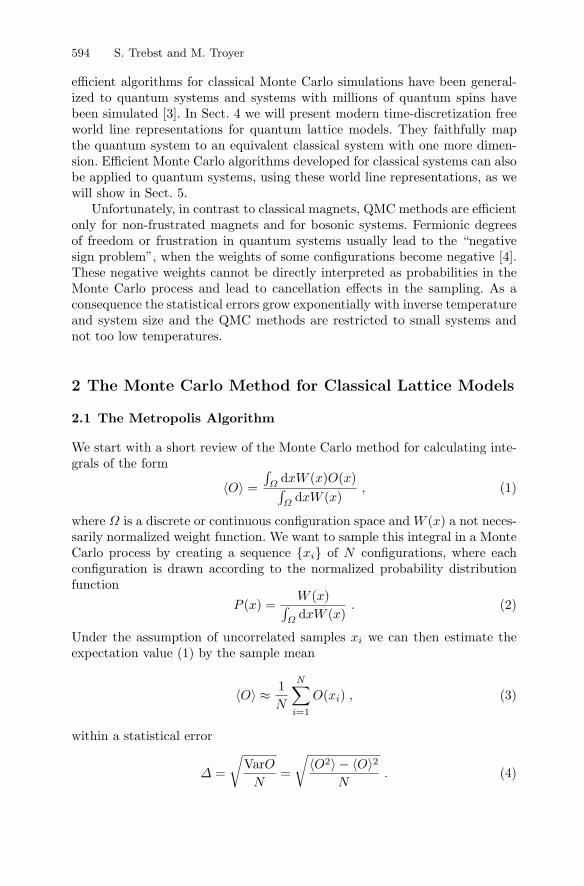
Under the assumption of uncorrelated samples xi we can then estimate theexpectation value (1) by the sample mean
〈O〉 ≈ 1N
N∑
i=1
O(xi) , (3)
within a statistical error
∆ =
√VarON
=
√〈O2〉 − 〈O〉2
N. (4)

Classical and Quantum Ensemble Optimization Techniques 595
Since we will, in general, not have a direct algorithm to create samplesxi according to the distribution P (xi) we will use a Markov process in whichstarting from an initial configuration x0 a Markov chain of configuration isgenerated:
x0 → x1 → x2 → . . . → xn → xn+1 → . . . . (5)
A transition matrix Txy gives the transition probabilities of going from config-uration x to configuration y in one step of the Markov process. As the sum ofprobabilities of going from configuration x to any other configuration is one,the columns of the matrix T are normalized:
∑
y
Txy = 1 . (6)
A consequence is that the Markov process conserves the total probability.Another consequence is that the largest eigenvalue of the transition matrixT is 1 and the corresponding eigenvector with only positive entries is theequilibrium distribution which is reached after a large number of Markovsteps.
We want to determine the transition matrix T so that we asymptoticallyreach the desired probability P (x) for a configuration i. A set of sufficientconditions is:
1. Ergodicity: It has to be possible to reach any configuration x from anyother configuration y in a finite number of Markov steps. This means thatfor all x and y there exists a positive integer n < ∞ such that (Tn)xy = 0.
2. Detailed balance: The probability distribution p(n)x changes at each step
of the Markov process:∑
x
p(n)x Txy = p(n+1)
y , (7)
but converges to the equilibrium distribution px. This equilibrium dis-tribution px is an eigenvector with left eigenvalue 1 and the equilibriumcondition ∑
x
pxTxy = py (8)
must be fulfilled. It is easy to see that the detailed balance condition
Wxy
Wyx=
py
px(9)
is sufficient.
The simplest Monte Carlo algorithm is the Metropolis algorithm [5] whichcan be outlined as follows:
• Starting with a configuration x = xi propose a new configuration y withan a-priori probability Axy.

596 S. Trebst and M. Troyer
• Calculate the acceptance ratio
Pxy = min(
1,AyxW (y)AxyW (x)
)(10)
and accept the proposed configuration with probability Pxy. To do so wedraw a uniform random number u in the interval [0, 1[ and choose xi+1 = yif u < Pxy and xi+1 = x otherwise.
• Measure the quantity O for the new configuration xi+1 no matter whetherthe proposed configuration was accepted or not.
Since the samples created in this Markov chain are correlated (we only dosmall changes at each step), equation (4) for the statistical error needs to bemodified to
∆ =
√VarON
(1 + 2τO) (11)
where τO is the integrated autocorrelation time of O(xi) in the Markov chain.
2.2 The Local Update Metropolis Algorithm for the Ising Model
We will next apply this Metropolis algorithm to simulations of the Ising fer-romagnet with Hamilton function
H = −J∑
〈i,j〉σiσj − gµBh
N∑
i=1
σi , (12)
where J is the exchange constant, h the magnetic field, g the Lande g-factor,µB the Bohr magneton, and N the total number of spins. The sum runs overall pairs of nearest neighbors i and j and σi = ±1 is the value of the Isingspin at site i.
To calculate the value of an observable, such as the mean magnetizationat an inverse temperature β = 1/kBT with T being the temperature and kB
the Boltzmann constant, we need to evaluate
〈m〉 =∑
c
m(c) exp(−βE(c))/Z, (13)
where
m(c) =1N
N∑
i=1
σi (14)
is the magnetization of the configuration c, E(c) the energy of the configura-tion,
P (c) = exp(−βE(c)) (15)
the Boltzmann weight and

Classical and Quantum Ensemble Optimization Techniques 597
Z =∑
c
P (c) (16)
the partition function, normalizing the weights.As discussed above, Monte Carlo sampling can be performed on this sum
using the Metropolis method. The simplest types of updates are local spinflips:
1. Pick a random site i. The a-priori probabilites Axy are all just 1/Nsites
for a system with Nsites spins.2. Calculate the energy cost ∆E for flipping the spin at site i: σi → −σi
3. Flip the spin with the Metropolis probability min[1, exp(−β∆E)]. If re-jected, keep the original spin value.
4. Perform a measurement independent of whether the spin flip was acceptedor rejected.
The same local update algorithm can be applied to systems with longer-range interactions and with coupling constants that vary from bond to bond.For more complex classical models, such as Heisenberg models, local updateswill no longer consist of simple spin flips, but of arbitrary rotations of thelocal spin vectors.
2.3 Critical Slowing Down and Cluster Update Algorithms
Local update algorithms are easy to implement and work well away from phasetransitions. Problems arise in the vicinity of continuous (second order) phasetransitions, where these algorithms suffer from “critical slowing down” [6] andat first order phase transitions where there is a tunneling problem throughfree energy barriers.
At second order phase transitions the correlation length ξ diverges uponapproaching the phase transition, and this causes the autocorrelation timesτO to also diverge as
τO ∝ min(L, ξ)z (17)
with a dynamical critical exponent of z ≈ 2. L is the linear extent of thesystem. The origin of critical slowing down is the fact that close to the criticaltemperature large ordered domains of linear extent ξ are formed and the sin-gle spin updates are not effective in changing these large domains. The valuez ≈ 2 can be understood considering that the time for a domain wall to movea distance ξ by a random walk scales as ξ2. The solution to critical slowingdown are cluster updates, flipping carefully selected clusters of spins instead ofsingle spins. Cluster update algorithms were originally invented by Swendsenand Wang for the Ising model [6] and soon generalized to O(N) models, suchas the Heisenberg model [7]. These cluster update algorithms are discussed intext books on classical Monte Carlo simulations and in computational physicstext books. While most cluster algorithms require spin-inversion invarianceand thus do not allow for external magnetic fields, extensions to spin models

598 S. Trebst and M. Troyer
in magnetic fields have been proposed [8,9]. An open source implementation oflocal and cluster updates for Ising, Potts, XY and Heisenberg models is avail-able through the ALPS (Applications and Libraries for Physics Simulations)project [10] at the web page http://alps.comp-phys.org/.
The tunneling problem at first order phase transitions and for disorderedsystems, where tunneling times often diverge exponentially can be overcomeusing extended ensemble methods, which are the main topic of the nextchapter.
3 Extended Ensemble Methods
3.1 First Order Phase Transitionsand the Multicanonical Ensemble
While cluster updates can solve critical slowing down at second order phasetransitions they are usually inefficient at first order phase transitions and infrustrated systems. Let us consider a first order phase transition, such as in atwo-dimensional q-state Potts model with Hamilton function
H = −J∑
〈i,j〉δσiσj
, (18)
where the spins σi can now take the integer values 1, . . . , q. For q > 4 thismodel exhibits a first order phase transition, accompanied by exponentialslowing down of conventional local update algorithms. The exponential slow-down is caused by the free energy barrier between the two coexisting meta-stable states at the first order phase transition.
This barrier can be quantified by considering the energy histogram
Hcanonical(E) ∝ g(E)PBoltzmann(E) = g(E) exp(−βE) , (19)
which is the probability of encountering a configuration with energy E duringthe Monte Carlo simulation. Here
g(E) =∑
c
δE,E(c) (20)
is the density of states. Away from first order phase transitions, Hcanonical(E)has approximately Gaussian shape, centered around the mean energy. At firstorder phase transitions, where the energy jumps discontinuously the histogramHcanonical(E) develops a double-peak structure. The minimum of Hcanonical(E)between these two peaks, which the simulation has to cross in order to gofrom one phase to the other, becomes exponentially small upon increasing thesystem size. This leads to exponentially large autocorrelation times.

Classical and Quantum Ensemble Optimization Techniques 599
This tunneling problem at first-order phase transitions can be relievedby extended ensemble techniques which aim at broadening the sampled en-ergy space. Instead of weighting a configuration c with energy E = E(c) us-ing the Boltzmann weight PBoltzmann(E) = exp(−βE) more general weightsPextended(E) are introduced which define the extended ensemble. The config-uration space is explored by generating a Markov chain of configurations
c1 → c2 → . . . → ci → ci+1 → . . . , (21)
where a move from configuration c1 to c2 is accepted with probability
Pacc(c1 → c2) = min(
1,P (c2)P (c1)
)= min
(1,
Wextended(E2)Wextended(E1)
). (22)
In general, the extended weights are defined in a single coordinate, such asthe energy, thereby projecting the random walk in configuration space to arandom walk in energy space
E1 = E(c1) → E2 → . . . → Ei → Ei+1 → . . . . (23)
For this random walk in energy space a histogram can be recorded which hasthe characteristic form
Hextended(E) ∝ g(E)Wextended(E) , (24)
where the density of states g(E) is fixed for the simulated system.One choice of generalized weights is the multicanonical ensemble [11, 12]
where the weight of a configuration c is defined as Wmulticanonical(c) ∝1/g(E(c)). The multicanonical ensemble then leads to a flat histogram inenergy space
Hmulticanonical(E) ∝ g(E)Wmulticanonical(E) = g(E)1
g(E)= const., (25)
removing the exponentially small minimum in the canonical distribution. Af-ter performing a simulation, measurements in the multicanonical ensemble arereweighted by a factor WBoltzmann(E)/Wmulticanonical(E) to obtain averages inthe canonical ensemble.
3.2 The Wang-Landau Algorithm
Since the density of states and thus the multicanonical weights are not knowninitially, a scalable algorithm to estimate these quantities is needed. TheWang-Landau algorithm [13, 14] is a simple but efficient iterative methodto obtain good approximations of the density of states g(E) and the multi-canonical weights Wmulticanonical(E) ∝ 1/g(E).
The algorithm starts with a (very bad) estimate of the density of statesg(E) = 1 for all energies which is iteratively improved by a modification factorf in the following loop:

600 S. Trebst and M. Troyer
• Start with g(E) = 1 and a modification factor f ≈ exp(1).• Repeat
– Reset a histogram of energies H(E) = 0.– Perform simulations until the histogram of energies H(E) is “flat”:
• Pick a random site and propose a local update, e.g. by flipping thespin at the site, which changes the current configuration c to a newconfiguration c′, and the energy from E = E(c) to E′ = E(c′).
• Approximating multicanoncal weights with the current estimateof the density of states the update is accepted with probabilitymin[1, g(E)/g(E′)].
• Increase the histogram at the current value of E: H(E) ← H(E)+1• Increase the estimate g(E) at the current value of E: g(E) ← fg(E).
– Once H(E) is “flat” and has “sufficient statistics”, reduce f ←√f .
• Stop once f is sufficiently small, e.g. f ≈ exp(10−6).
Only a few lines of code need to be changed in the local update algorithmfor the Ising model, but a few remarks are helpful:
1. The initial value for f needs to be carefully chosen, f = exp(1) is only arough guide. A good choice is picking the initial f such that fNsweeps isapproximately the total number of states
∑E g(E) (e.g. 2N for an Ising
model with N sites).2. Checking for flatness of the histogram (e.g. the minimum is at least 80%
of the mean) should be done only after a reasonable number of sweepsNsweeps. One sweep is defined as one attempted update per site.
3. The flatness criterion is quite arbitrary. In order to ensure convergence ofthe estimated g(E) it should be extended to enforce sufficient statistics,e.g. by requiring that each histogram entry is at least of the order of1/√
ln f as pointed out in Refs. [15,16].4. The density of states g(E) can become very large and easily exceed 1010000.
In order to obtain such large numbers the multiplicative increase g(E) ←fg(E) is essential. A naive additive guess g(E) ← g(E) + f would neverbe able to reach the large numbers needed.
5. Since g(E) is so large, we only store its logarithm. The update step is thusln g(E) ← ln g(E) + ln f .
At the end, the density of states g(E) needs to be normalized. Either aknown ground state degeneracy (e.g. g(EGS) = 2 in the Ising ferromagnet) ora known total number of states (e.g.
∑E g(E) = 2N in the Ising model with
N spins) or a combination of the two (e.g. g(EGS) ·∑
E g(E) = 2N+1 for theIsing ferromagnet) can be used to normalize g(E).
Besides overcoming the exponentially suppressed tunneling problem atfirst order phase transitions, the Wang-Landau algorithm calculates the gen-eralized density of states g(E) in an iterative procedure. The knowledge ofthe density of states g(E) then allows the direct calculation of the free energyfrom the partition function (16). The internal energy, entropy, specific heat

Classical and Quantum Ensemble Optimization Techniques 601
and other thermal properties are easily obtained as well, by differentiating thefree energy. By additionally measuring the averages A(E) of other observablesA as a function of the energy E, thermal expectation values can be obtainedat arbitrary inverse temperatures β by performing just a single simulation:
〈A(β)〉 =∑
E A(E)g(E)e−βE
∑E g(E)e−βE
. (26)
3.3 Markov Chains and Random Walks in Energy Space
The multicanonical ensemble and Wang-Landau algorithm both project a ran-dom walk in high-dimensional configuration space onto a one-dimensional ran-dom walk in energy space where all energy levels are sampled equally often.It is important to note that the random walk in configuration space, (21), isa biased Markovian random walk, while the projected random walk in energyspace, (23), is non-Markovian, as memory is stored in the configuration. Thisbecomes evident as the system approaches a phase transition in the randomwalk: While the energy no longer reflects from which side the phase transitionis approached, the current configuration may still reflect the actual phase thesystem has visited most recently. In the case of the two-dimensional ferro-magnetic Ising model, the order parameter for a given configuration at thecritical energy Ec ∼ −1.41N will reveal whether the system is approachingthe transition from the magnetically ordered (lower energies) or disorderedside (higher energies).
This loss of information in the projection of the random walk in configura-tion space has important consequences for the random walk in energy space.Most strikingly, the local diffusivity of a random walker in energy space, whichfor a diffusion time tD can be defined as
D(E, tD) = 〈(E(t) − E(t + tD))2〉/tD (27)
is not independent of the location in energy space. This is illustrated in Fig. 1for the Ising ferromagnet. Below the phase transition around E ∼ −1.41Na clear minimum evolves in the local diffusivity. In this region large ordereddomains are formed and by moving the domain boundaries through local spinflips only small energy changes are induced resulting in a suppressed localdiffusivity in energy space.
Because of the strong energy dependence of the local diffusivity the sim-ulation of a multicanonical ensemble sampling all energy levels equally oftenturns out to be suboptimal [17]. The performance of flat-histogram algorithmscan be quantified for classical spin models such as the ferromagnet where thenumber of energy levels is given by [−2N,+2N ] and thereby scales with thenumber of spins N in the system. When measuring the typical round-triptime between the two extremal energies for multicanonical simulations, theseround-trip times τ are found to scale like

602 S. Trebst and M. Troyer
-1 -0.9 -0.8 -0.7 -0.6 -0.5 -0.4 -0.3 -0.2 -0.1 0E / 2N
1
2
3
4
5
loca
l dif
fusi
vity
Fig. 1. Local diffusivity D(E, tD) = 〈(E(t) − E(t + tD))2〉/tD of a random walksampling a flat histogram in energy space for the two-dimensional ferromagneticIsing model. The local diffusivity strongly depends on the energy with a strongsuppression below the critical energy Ec ≈ −1.41 N
τ ∼ N2Lz , (28)
showing a power-law deviation from the N2-scaling behavior of a completelyunbiased random walk. Here z is a critical exponent describing the slowdown ofa multicanonical simulation in the proximity of a phase transition [17,18]. Thevalue of z strongly depends on the simulated model and the dimensionality ofthe problem. In two dimensions the exponent increases from z = 0.74 for theferromagnet as one introduces competing interactions leading to frustrationand disorder. The exponent becomes z = 1.73 for the fully frustrated Isingmodel which is defined by a Hamilton
H =∑
〈i,j〉Jijσiσj , (29)
where the spins around any given plaquette of four spins are frustrated, e.g.by choosing the couplings along three bonds to be Jij = −1 (ferromagnetic)and Jij = +1 (antiferromagnetic) for the remaining bond. For the spin glasswhere the couplings Jij are randomly chosen to be +1 or −1 exponentialscaling (z = ∞) is found [17, 19]. Increasing the spatial dimension for theferromagnet the exponent is found to decrease as z ≈ 1.81, 0.74 and 0.44 fordimension d = 1, 2 and 3 and z vanishes for the mean-field model in the limitof infinite dimensions [18].

Classical and Quantum Ensemble Optimization Techniques 603
3.4 Optimized Ensembles
The observed polynomial slowdown for the multicanonical ensemble poses thequestion whether for a given model there is an optimal choice of sampling en-ergies, Hoptimal(E) and corresponding weights Woptimal(E), which eliminatesthe slowdown. To address this question an adaptive feedback algorithm hasrecently been introduced that iteratively improves the weights in an extendedensemble simulationt leading to further improvements in the efficiency of thealgorithm by several orders of magnitude [20]. The scaling for the optimizedensemble is found to scale like O([N lnN ]2) thereby reproducing the behaviorof an unbiased Markovian random walk up to a logarithmic correction.
At the heart of the algorithm is the idea to maximize a current j of walk-ers that move from the lowest energy level, E−, to the highest energy level,E+, or vice versa, in an extended ensemble simulation by varying the weightsWextended(E). To measure the current a label is added to the walker thatindicates which of the two extremal energies the walker has visited most re-cently. The two extrema act as “reflecting” and “absorbing” boundaries forthe labeled walker: e.g., if the label is plus, a visit to E+ does not change thelabel, so this is a “reflecting” boundary. However, a visit to E− does changethe label, so the plus walker is absorbed at that boundary. The behavior ofthe labeled walker is not affected by its label except when it visits one of theextrema and the label changes.
For the random walk in energy space, two histograms are recorded, H+(E)and H−(E), which for sufficiently long simulations converge to steady-statedistributions which satisfy H+(E) + H−(E) = H(E) = W (E)g(E). For eachenergy level the fraction of random walkers which have label “plus” is thengiven by f(E) = H+(E)/H(E). The above-discussed boundary conditionsdictate f(E−) = 0 and f(E+) = 1.
The steady-state current to first order in the derivative is
j = D(E)H(E)df
dE, (30)
where D(E) is the walker’s diffusivity at energy E. There is no current if f(E)is constant, since this is equilibrium. Therefore the current is to leading orderproportional to df/dE. Rearranging the above equation and integrating onboth sides, noting that j is a constant and f runs from 0 to 1, one obtains
1j
=∫ E+
E−
dE
D(E)H(E). (31)
To maximize the current and thus the round-trip rate, this integral must beminimized. However, there is a constraint: H(E) is a probability distributionand must remain normalized which can be enforced with a Lagrange multi-plier: ∫ E+
E−
dE
(1
D(E)H(E)+ λH(E)
). (32)

604 S. Trebst and M. Troyer
To minimize this integrand, the ensemble, that is the weights W (E) andthus the histogram H(E) are varied. At this point it is assumed that thedependence of D(E) on the weights can be neglected.
The optimal histogram, Hoptimal(E), which minimizes the above integrandand thereby maximizes the current j is then found to be
Hoptimal(E) ∝ 1√D(E)
. (33)
Thus for the optimal ensemble, the probability distribution of sampled energylevels is simply inversely proportional to the square root of the local diffusivity.
The optimal histogram can be approximated in a feedback loop of theform
• Start with some trial weights W (E), e.g. W (E) = 1/g(E).• Repeat
– Reset the histograms H(E) = H+(E) = H−(E) = 0.– Simulate the system with the current weights for N sweeps:
• Updates are accepted with probablity min[1,W (E′)/W (E)].• Record the histograms H+(E) and H−(E).
– From the recorded histogram an estimate of the local diffusivity isobtained as
D(E) ∝ 1H(E) df
dE
, f(E) =H+(E)H(E)
, H(E) = H+(E)+H−(E) .
– Define new weights as
Woptimized(E) = W (E)
√1
H(E)· df
dE.
– Increase the number of sweeps for the next iteration N ← 2N .• Stop once the histogram H(E) has converged.
Again the implementation of this feedback algorithm requires to changeonly a few lines of code in the original local update algorithm for the Isingmodel. Some additional remarks are useful:
1. In contrast to the Wang-Landau algorithm the weights W (E) are modifiedonly after a batch of N sweeps, thereby ensuring detailed balance betweensuccessive moves at all times.
2. The initial value of sweeps N should be chosen large enough that a coupleof round trips are recorded, thereby ensuring that steady state data forH+(E) and H−(E) are measured.
3. The derivative df/dE can be determined by a linear regression, where thenumber of regression points is flexible. Initial batches with the limited sta-tistics of only a few round trips may require a larger number of regressionpoints than subsequent batches with smaller round-trip times and betterstatistics.

Classical and Quantum Ensemble Optimization Techniques 605
4. Similar to the multicanonical ensemble the weights W (E) can become verylarge, and storing the logarithms may be advantageous. The reweightingthen becomes lnWoptimized(E) = lnW (E) + (ln df
dE − lnH(E))/2 .
At the end of the simulation, the density of states can be estimated fromthe recorded histogram as g(E) = Hoptimized(E)/Woptimized(E) and normal-ized as described above.
Figure 2 shows the optimized histogram for the two-dimensional ferro-magnetic Ising model. The optimized histogram is no longer flat, but a peakevolves at the critical region around Ec ≈ −1.41 N of the transition. Thefeedback of the local diffusivity reallocates resources towards the bottlenecksof the simulation which have been identified by a suppressed local diffusivity.
The scaling of round-trip times is shown in Fig. 3 for the two-dimensionalfully frustrated Ising model. The power-law slowdown of round-trip times forthe flat-histogram ensemble O(N2L1.73) is reduced to a logarithmic correctionO([N lnN ]2) for the optimized ensemble in comparison to a completely unbi-ased random walk with O(N2)-scaling. This scaling improvement results in aspeedup by a nearly two orders of magnitude already for a system with some128 × 128 spins.
-1 -0.9 -0.8 -0.7 -0.6 -0.5 -0.4 -0.3 -0.2 -0.1 0E / 2N
0
1
2
3
hist
ogra
m
Fig. 2. Optimized histograms for the two-dimensional ferromagnetic Ising model.After the feedback of the local diffusivity a peak evolves near the critical energyof the transition Ec ≈ −1.41 N . The feedback thereby shifts additional resourcestowards the bottleneck of the simulation which were identified by a suppressed localdiffusivity

606 S. Trebst and M. Troyer
8 16 32 64 128
L = N 1 / 2
0.1 0.1
1 1
10 10
100 100
τ / N
2
optimized ensemble
flat-histogram ensemble
Fig. 3. Scaling of round-trip times for a random walk in energy space sampling aflat histogram (open squares) and the optimized histogram (solid circles) for the two-dimensional fully frustrated Ising model. While for the multicanonical simulation apower-law slowdown of the round-trip times O(N2Lz) is observed, the round-triptimes for the optimized ensemble scale like O([N ln N ]2) thereby approaching theideal O(N2)-scaling of an unbiased Markovian random walk up to a logarithmiccorrection
3.5 Simulation of Dense Fluids
Extended ensembles cannot only be defined as a function of energy, but inarbitrary reaction coordinates R onto which a random walk in configurationspace can be projected. The generalized weights in these reaction coordinatesWextended(R) are then used to bias the random walk along the reaction coor-dinate by accepting moves from a configuration c1 with reaction coordinateR1 to a configuration c2 with reaction coordinate R2 with probability
pacc(c1 → c2) = pacc(R1 → R2) = min(
1,Wextended(R2)Wextended(R1)
). (34)
The generalized weights Wextended(R) can again be chosen in such a way thatsimilar to a multicanonical simulation a flat histogram is sampled along thereaction coordinate by setting the weights to be inversely proportional to thedensity of states defined in the reaction coordinates, that is Wextended(R) ∝1/g(R).
An optimal choice of weights can be found by measuring the local dif-fusivity of a random walk along the reaction coordinates and applying thefeedback method to shift weight towards the bottlenecks in the simulation.This generalized ensemble optimization approach has recently been illustratedfor the simulation of dense Lennard-Jones fluids close to the vapor-liquid equi-librium [21]. The interaction between particles in the fluid is described by a

Classical and Quantum Ensemble Optimization Techniques 607
pairwise Lennard-Jones potential of the form
ΦLJ(R) = 4ε[( σ
R
)12−( σR
)6], (35)
where ε is the interaction strength, σ a length parameter, and R the distancebetween two particles. It is this distance R between two arbitrarily chosen par-ticles in the fluid that one can use as a new reaction coordinate for a projectedrandom walk. Defining an extended ensemble with weights Wextended(R) andrecording a histogram H(R) during a simulation will then allow to calculatethe pair distribution function g(R) = H(R)/Wextended(R). The pair distribu-tion function g(R) is closely related to the potential of mean force (PMF)
ΦPMF(R) = − 1β
ln g(R) , (36)
which describes the average interaction between two particles in the fluid inthe presence of many surrounding particles.
For high particle densities and low enough temperatures shell structureswill form in the fluid which are reminiscent of the hexagonal lattice of the solidstructure at very low temperatures. These shell structures are revealed by asinusoidal modulation in the PMF as illustrated in the lower panel of Fig. 4 forthe case of a two-dimensional fluid. Thermal equilibration between the shells issuppressed by entropic barriers which form between the shells. Again, one canask what probability distribution, or histogram, should be sampled along thereaction coordinate, in this case the radial distance R, so that equilibrationbetween the shells is improved. Measuring the local diffusivity for a randomwalk along the radial distance R in an interval [Rmin, Rmax] and subsequentlyapplying the feedback algorithm described above optimized histograms H(R)are found which are plotted in Fig. 4 for varying temperatures [21]. The feed-back algorithm again shifts additional weight in the histogram towards thebottleneck of the simulation, in this case towards the barriers between theshells. Interestingly, additional peaks emerge in the optimized histogram asthe temperature is lowered towards the vapor-liquid equilibrium. The minimabetween these peaks points to additional meta-stable configurations which oc-cur at these low temperatures, namely interstitial states which occur as theshells around two particles merge as detailed in [21].
This example illustrates that for some simulations the local diffusivity andoptimized histogram itself are very sensitive measures that can reveal interest-ing phenomena which are otherwise hard to detect in a numerical simulation.In general, a strong modulation of the local diffusivity for the random walkalong a given reaction coordinate is a good indicator that the reaction co-ordinate itself is a good choice that captures some interesting physics of theproblem.

608 S. Trebst and M. Troyer
0
0.01
0.02
0.03
0.04
0.05
0.06
hist
ogra
m
T = 0.500T = 0.575T = 0.750T = 1.000T = 3.000
1 2 3 4 5 6R/σ
-2
0
2
ΦPM
F(R) T = 0.500
T = 3.000
Fig. 4. Optimized histograms for the simulation of dense Lennard-Jones fluids
3.6 Parallel Tempering
The simulation of frustrated systems suffers from a similar tunneling problemas the simulation of first order phase transitions: local minima in energy spaceare separated by barriers that grow with system size. While the multicanonicalor optimized ensembles do not help with the NP-hard problems faced by spinglasses, they are efficient in speeding up simulations of frustrated magnetswithout disorder.
An alternative to these extended ensembles for the simulation of frus-trated magnets is the “parallel tempering” or “replica exchange” Monte Carlomethod [22–25]. Instead of performing a single simulation at a fixed tem-perature, simulations are performed for M replicas at a set of temperaturesT1, T2, . . . , TM . In addition to standard Monte Carlo updates at a fixed tem-perature, exchange moves are proposed to swap two replicas between adjacenttemperatures. These swaps are accepted with a probability
min[1, exp(∆β∆E)], (37)
where ∆β is the difference in inverse temperatures and ∆E the difference inenergy between the two replicas.
The effect of these exchange moves is that a replica can drift from a localfree energy minimum at low temperatures to higher temperatures, where itis easier to cross energy barriers and equilibration is fast. Upon cooling (byanother sequence of exchanges) it can end up in a different local minimum ontime scales that are much shorter compared to a single simulation at a fixedlow temperature. This random walk of a single replica in temperature spaceis the analog of the random walk in energy space discussed for the extended

Classical and Quantum Ensemble Optimization Techniques 609
ensemble techniques. The complement of the statistical ensemble, defined bythe weights Wextended(E), is the particular choice of temperature points in thetemperature set T1, T2, . . . , TM for the parallel tempering simulation. Theprobability of sampling any given temperature T in an interval Ti < T < Ti+1
can then be approximated by H(T ) ∝ 1/∆T , where ∆T = Ti+1 − Ti is thelength of the temperature interval around the temperature T . This probabilitydistribution H(T ) is the equivalent to the histogram H(E) in the extendedensemble simulations. The ensemble optimization technique introduced abovecan thus be reformulated to optimize the temperature set in a parallel tem-pering simulation in such a way that the rate of round-trips between the twoextremal temperatures, T1 and TM respectively, is maximized [26,27].
Starting with an initial temperature set T1, T2, . . . , TM a parallel tem-pering simulation is performed where each replica is labeled either “plus” or“minus” indicating which of the two extremal temperatures the respectivereplica has visited most recently. This allows to measure a current of replicasdiffusing from the highest to the lowest temperature by recording two his-tograms, h+(T ) and h−(T ) for each temperature point. The current j is thengiven by
j = D(T )H(T )df
dT, (38)
where D(T ) is the local diffusivity for the random walk in temperature space,and f(T ) = h+(T )/(h+(T ) + h−(T )) is the fraction of random walkers whichhave visited the highest temperature TM most recently. The probability dis-tribution H(T ) is normalized, that is
∫ TM
T1
H(T ) dT = C
∫ TM
T1
dT
∆T= 1 , (39)
where C is a normalization constant. Rearranging (38) the local diffusivityD(T ) of the random walk in temperature space can be estimated as
D(T ) ∝ ∆T
df/dT. (40)
Analog to the argument for the extended ensemble in energy space the currentj is maximized by choosing a probability distribution
Hoptimal(T ) ∝ 1√D(T )
∝√
1∆T
df
dT(41)
which is inversely proportional to the square root of the local diffusivity. Theoptimized temperature set T ′
1, T′2, . . . , T
′M is then found by choosing the
n-th temperature point T ′n such that
∫ T ′n
T ′1
Hoptimal(T ) dT =n
M, (42)

610 S. Trebst and M. Troyer
where M is the number of temperature points in the original temperature set,and the two extremal temperatures T ′
1 = T1 and T ′M = TM remain unchanged.
Similarly to the algorithm for the ensemble optimization this feedback of thelocal diffusivity should be iterated until the temperature set is converged.
Figure 5 illustrates the optimized temperature sets for the Ising ferromag-net obtained by several iterations of the above feedback loop. After feedbackof the local diffusivity temperature points accumulate near the critical tem-perature Tc = 2.269 of the transition. This is in analogy to the optimized his-tograms for the extended ensemble simulations where resources where shiftedtowards the critical energy of the transition, see Fig. 2.
It is interesting to note that for the optimized temperature set the accep-tance rates for swap moves are not independent of the temperature. Aroundthe critical temperature, where temperature points are accumulated by thefeedback algorithm, the acceptance rates are higher as at higher/lower temper-atures, where the density of temperature points becomes considerably smallerafter feedback. The almost Markovian scaling behavior for the optimizedrandom walks in either energy or temperature space is thus generated bya problem-specific statistical ensemble which is characterized neither by a flathistogram nor flat acceptance rates for exchange moves, but by a characteristic
0 2 4 6 8 10temperature T
0
1
2
3
4
feed
back
iter
atio
n
critical temperatureT
c=2.269
Fig. 5. Optimized temperature sets for the two-dimensional Ising ferromagnet. Theinitial temperature set with 20 temperature points is determined by a geometric pro-gression for the temperature interval [0.1, 10]. After feedback of the local diffusivitythe temperature points accumulate near the critical temperature Tc = 2.269 of thephase transition (dashed line). Similar to the ensemble optimization in energy spacethe feedback of the local diffusivity relocates resources towards the bottleneck of thesimulation

Classical and Quantum Ensemble Optimization Techniques 611
Fig. 6. Low-energy structure of the 36-residue chicken villin headpiece sub-domainHP-36. On the left the structure determined in NMR experiments is shown. Theright panel shows the lowest-energy configuration found in a feedback-optimized all-atom parallel tempering simulation using the ECEPP/2 force field and an implicitsolvent model. The root-mean square deviation of this structure to the structure onthe left is RRMSD = 3.8 A
probability distribution which concentrates resources at the minima of themeasured local diffusivity.
3.7 Optimized Parallel Tempering Simulations of Proteins
The feedback-optimized parallel tempering technique [26] outlined in the pre-vious section has recently been applied to study the folding of the 36-residuechicken villin headpiece sub-domain HP-36 [27]. Since HP-36 is one of thesmallest proteins with well-defined secondary and tertiary structure [28] andat the same time with 596 atoms still accessible to numerical simulations, ithas recently attracted considerable interest as an example to test novel numer-ical techniques, including molecular dynamics [29,30] and Monte Carlo [31,32]methods. The experimentally determined structure [28] which is deposited inthe Protein Data Bank (PDB code 1vii) is illustrated in the left panel of Fig. 6.
Applying an all-atom parallel tempering simulation of the protein HP-36in the ECEPP/2 force field [33] using an implicit solvent model [34] the au-thors of [27] have measured the diffusion of labeled replicas in temperaturespace. The simulated temperature interval is chosen such that at the lowesttemperature Tmin = 250 K the protein is in a folded state and the highesttemperature Tmax = 1000 K ensures that the protein can fully unfold forthe simulated force field. The measured local diffusivity for the random walkbetween these two extremal temperatures is shown in Fig. 7. A very strongmodulation of the local diffusivity is found along the temperature. Note thelogarithmic scale of the ordinate. The pronounced minimum of the local diffu-sivity around T ≈ 500 K points to a severe bottleneck in the simulation whichby measurements of the specific heat has been identified as the helix-coil

612 S. Trebst and M. Troyer
300 400 500 600 700
temperature T [K]
103
104
105
106
107
loca
l dif
fusi
vity
D(T
)
0
5
10
15
20
spec
ific
hea
t C
V (
T)
Fig. 7. Local diffusivity (solid circles) of the random walk in temperature spacefor a parallel tempering simulation of the 36-residue villin headpiece sub-domainHP-36. The diffusivity shows a strong modulation along the temperature, note thelogarithmic scale of the ordinate. Slightly below the helix-coil transition aroundT ≈ 500 K which is identified by a maximum in the specific heat (crosses, rightordinate) there is a strong suppression of the diffusivity
transition [31]. Above this transition the protein is in an extended unorderedconfiguration, while below the helix-coil transition the protein is character-ized by high helical content [31]. The shoulder in the local diffusivity in thetemperature region 350 K ≤ T ≤ 490 K points to a second bottleneck in thesimulation, possibly caused by competing low-energy configurations with highhelical content.
An optimized temperature set for the parallel tempering simulation of HP-36 in the ECEPP/2 force field can then be found by feeding back the local dif-fusivity applying the algorithm outlined above. Results for a temperature setwith 20 temperature points are illustrated in Fig. 8 for an initial temperatureset which similar to a geometric progression concentrates temperature pointsat low temperatures [27]. After the feedback temperature points concentratearound the bottleneck of the simulation, primarily around the helix-coil tran-sition at T ≈ 500 K and in the temperature regime 350 K ≤ T ≤ 490 K belowthe transition where a shoulder in the local diffusivity was found.
In [27] it was demonstrated that by using the optimized temperature set inthe simulations the low-energy configurations equilibrated considerably fasterthan in previous parallel tempering simulations [31]. As a consequence, thelow energy structures are more compact and the configuration with lowestenergy illustrated in Fig. 6 shows a root-mean square deviation to the exper-imentally determined structure of RRMSD = 3.7 A. This deviation from thenative structure is similar to results found by large-scale molecular dynamics

Classical and Quantum Ensemble Optimization Techniques 613
200 400 600 800 1000
temperature T [K]
0
1
2fe
edba
ck it
erat
ion
Fig. 8. Optimized temperature sets with 20 temperature points for the paralleltempering simulation of the 36-residue protein HP-36. The initial temperature setcovers a temperature range 250 K ≤ T ≤ 1000 K and concentrates temperaturepoints at low temperatures similar to a geometric progression. After the feedback ofthe local diffusivity temperature points accumulate around the helix-coil transitionat T ≈ 500 K where the strong suppression of the local diffusivity points to a severebottleneck
simulations [30] with a different force field. However, employing the optimizedtemperature set the Monte Carlo simulations consumed only a fraction of onepercent of the computing time used for the molecular dynamics simulations.A detailed discussion of the application of the feedback method in the studyof proteins is given in [27].
3.8 Simulation of Quantum Systems
Extended ensemble methods, such as the multicanonical ensemble, Wang-Landau sampling or parallel tempering can also be generalized to quantumsystems [35,36], as we will show in the next two sections.
4 Quantum Monte Carlo World Line Algorithms
4.1 The S = 1/2 Quantum XXZ Model
In this section we will generalize the Monte Carlo methods described in section2 for classical spin systems to quantum spin systems. As an example we willuse the spin-1/2 quantum Heisenberg or XXZ models with Hamiltonian

614 S. Trebst and M. Troyer
H =∑
〈i,j〉
[JzS
zi S
zj + Jxy
(Sx
i Sxj + Sy
i Syj
)]− h
N∑
i=1
Szi (43)
=∑
〈i,j〉
[JzS
zi S
zj +
Jxy
2(S+
i S−j + S−
i S+j
)]− h
N∑
i=1
Szi
where Sαi are spin S = 1/2 operators fulfilling the standard commutation
relations and in the second line we have replaced Sxi and Sy
i by the spinraising and lowering operators S+
i and S−i .
The case Jxy = 0 corresponds to the classical Ising model (12) up to achange in sign: while in classical Monte Carlo simulations (where there is nodifference in the thermodynamics of the ferromagnet and the antiferromagnet)a positive exchange constant J denotes the ferromagnet, the convention forquantum systems is usually opposite with a positive exchange constant denot-ing the antiferromagnet. The other limit Jz = 0 corresponds to the quantumXY -model, while Jz = Jxy is the Heisenberg model.
4.2 Representations
The basic problem for Monte Carlo simulations of quantum systems is thatthe partition function is no longer a simple sum over classical configurationsas in (16) but an operator expression
Z = Tr exp(−βH) , (44)
where H is the Hamilton operator and the trace Tr goes over all states in theHilbert space. Similarly the expression for an observable like the magnetizationis an operator expression:
〈m〉 =1Z
Tr [m exp(−βH)] , (45)
and the Monte Carlo method cannot directly be applied except in the classicalcase where the Hamilton operator H is diagonal and the trace reduces to asum over all basis states. The first step of any QMC algorithm is thus themapping of the quantum system to an equivalent classical system
〈m〉 =1Z
Tr [m exp(−βH)] =∑
c
m(c)W (C) , (46)
where the sum goes over configurations c in an artificial classical system (e.g. asystem of world lines), m(c) will be the value of the magnetization or anotherobservable as measured in this classical system and W (C) the weight of theclassical configuration. We will now present two different but related methodsfor this mapping, namely continuous time path integrals and the stochasticseries expansion.

Classical and Quantum Ensemble Optimization Techniques 615
The Path-Integral Representation
The path-integral formulation of a quantum systems goes back to [37], andforms the basis of most QMC algorithms. Instead of following the historicalroute and discussing the Trotter-Suzuki (checkerboard) decomposition [38,39]for path integrals with discrete time steps ∆τ we will directly describe thecontinuous-time formulation used in modern codes.
The starting point is a time-dependent perturbation expansion in imagi-nary time to evaluate the density matrix operator exp(−βH). Using a basis inwhich the Sz operators are diagonal we follow [40] and split the HamiltonianH = H0 +V into a diagonal term H0, containing the Sz term and an offdiag-onal perturbation V , containing the exchange terms (Jxy/2)(S+
i S−j +S−
i S+j ).
In the interaction representation the time-dependent perturbation is V (τ) =exp(τH0)V exp(−τH0) and the partition function can be represented as:
Z = Tr exp(−βH) = Tr
[exp(−βH0)T exp
∫ β
0
dτV (τ)
],
= Tr
[exp(−βH0)
(1 −∫ β
0
dτ1V (τ1) +1
2
∫ β
0
dτ1
∫ β
τ1
dτ2V (τ1)V (τ2) + . . .
)]
=∑
i
〈i|[exp(−βH0)
(1−∫ β
0
dτ1V (τ1)+1
2
∫ β
0
dτ1
∫ β
τ1
dτ2V (τ1)V (τ2) + . . .
)]|i〉,
(47)
where the symbol T denotes time-ordering of the exponential and in the lastline we have replaced the trace by a sum over a complete set of basis states|i〉, that are eigenstates of the local Sz operators. Note that, in contrast to areal time path integral, the imaginary time path integral always converges onfinite systems of N spins at finite temperatures β, and the expansion can betruncated at orders n βJxyN .
Equation (47) is now just a classical sum of integrals and can be evaluatedby Monte Carlo sampling in the intitial states |i〉, the order of the perturbationn and the times τi (i = 1, . . . , n). This is best done by considering a graphicalworld line representation of the partition function (47) shown in Fig. 9. Thezero-th order terms in the sum
∑i〈i| exp(−βH0)|i〉 are given by straight world
lines shown in Fig. 9a. First order terms do not appear since the matrixelements 〈i|V |i〉 are zero for the XXZ model. The first non-trivial termsappear in second order with two exchanges, as shown in Fig. 9b. A generalconfiguration of higher order is depicted in Fig. 10a.
Since the XXZ Hamiltonian commutes with the z-component of total spin∑i S
zi , the total magnetization is conserved and all valid configurations are
represented by closed world lines as shown in Figs. 9 and 10. Models thatbreak this conservation of magnetization, such as general XY Z models withdifferent couplings in all directions, models with transverse fields coupling toSx
i or higher spin models with single ion anisotropies (Sxi )2 or (Sy
i )2 will inaddition contain configurations with broken world line segments.

616 S. Trebst and M. Troyer
a) b)
space direction
imag
inar
y tim
e
0
β
space direction
imag
inar
y tim
e
0
β
τ1
τ2
Fig. 9. Examples of simple world line configurations in imaginary time for a quan-tum spin model. Up-spins are shown by bold lines and down spins by thin lines. (a)a configuration in 0-th order perturbation theory where the spins evolve accordingto the diagonal term exp(−βH0) and the weight is given by the classical Boltz-mann weight of H0. (b) a configuration in second order perturbation theory withtwo exchanges at times τ1 and τ2. Its weight is given by the matrix elements of theexchange processes and the classical Boltzmann weight of H0 of the spins
a)
space direction
inte
ger
inde
x
b)
1
n
space direction
imag
inar
y tim
e
0
β
Fig. 10. Examples of world line configurations in (a) a path-integral representationwhere the time direction is continuous and (b) the stochastic series expansion (SSE)representation where the “time” direction is discrete. Since the SSE representationperturbs not only in offdiagonal terms but also in diagonal terms, additional diagonalterms are present in the representation, indicated by dashed lines

Classical and Quantum Ensemble Optimization Techniques 617
The Stochastic Series Expansion Representation
An alternative representation is the stochastic series expansion (SSE) [41],a generalization of Handscomb’s algorithm [42] for the Heisenberg model. Itstarts from a Taylor expansion of the partition function in orders of β:
Z = Tr exp(−βH) =∞∑
n=0
βn
n!Tr(−H)n (48)
=∞∑
n=0
βn
n!
∑
i1,...in
∑
b1,...bn〈i1| −Hb1 |i2〉〈i2| −Hb2 |i3〉 · · · 〈in| −Hbn
|i1〉 ,
where in the second line we decomposed the Hamiltonian H into a sum ofsingle-bond terms H =
∑b Hb, and again inserted complete sets of basis
states. We end up with a similar representation as (47) and a related world-line picture shown in Fig. 10b.
The key difference is that the SSE representation is a perturbation expan-sion in all terms of the Hamiltonian, while the path-integral representationperturbs only in the off-diagonal terms. Although the SSE method thus needshigher expansion orders for a given system, this disadvantage is compensatedby a simplification in the algorithms: only integer indices of the operators needto be stored instead of continuous time variables τi. Except in strong magneticfields or for dissipative quantum spin systems [43,44] the SSE representationis thus the preferred representation for the simulation of quantum magnets.
The Negative Sign Problem
While the mapping from the quantum average to a classical average in (46) canbe performed for any quantum system, it can happen in frustrated quantummagnets, that some of the weights W (C) in the quantum system are negative,as is shown in Fig. 11.
Since Monte Carlo sampling requires positive weights W (C) > 0 the stan-dard way of dealing with the negative weights of the frustrated quantummagnets is to sample with respect to the unfrustrated system by using theabsolute values of the weights |W (C)| and to assign the sign, s(c) ≡ signW (C)to the quantity being sampled:
〈m〉 =∑
c m(c)W (C)∑c W (C)
=∑
c m(c)s(c)|W (C)| /∑
c |W (C)|∑c s(c)|W (C)| /
∑c |W (C)| ≡ 〈ms〉′
〈s〉′ . (49)
While this allows Monte Carlo simulations to be performed, the errors in-crease exponentially with the particle number N and the inverse temperatureβ. To see this, consider the mean value of the sign 〈s〉 = Z/Z ′, which is justthe ratio of the partition functions of the frustrated system Z =
∑c W (C)
with weights W (C) and the unfrustrated system used for sampling with

618 S. Trebst and M. Troyer
-Jxy/2
-Jxy/2
-Jxy/2
Fig. 11. Example of a frustrated world line configuration in a Heisenberg quantumantiferromagnet on a triangle. The closed world line configuration contains threeexchange processes, each contributing a weight proportional to −Jxy/2. The overallis proportional to (−Jxy/2)3 and is negative, causing a negative sign problem forthe antiferromagnet with Jxy > 0
Z ′ =∑
c |W (C)|. As the partition functions are exponentials of the corre-sponding free energies, this ratio is an exponential of the differences ∆f inthe free energy densities:〈s〉 = Z/Z ′ = exp(−βN∆f). As a consequence, therelative error ∆s/〈s〉 increases exponentially with increasing particle numberand inverse temperature:
∆s
〈s〉 =
√(〈s2〉 − 〈s〉2) /M
〈s〉 =
√1 − 〈s〉2√M〈s〉
∼ exp(βN∆f)√M
. (50)
Here M is the number of uncorrelated Monte Carlo samples. Similarly theerror for the numerator increases exponentially and the time needed to achievea given relative error scales exponentially in N and β.
It was recently shown that the negative sign problem is NP-hard, im-plying that almost certainly no solution for this exponential scaling problemexists [4]. Given this exponential scaling of quantum Monte Carlo simulationsfor frustrated quantum magnets, the QMC method is best suited for nonfrus-trated magnets and we will restrict ourselves to these sign problem free casesin the following.
Measurements
Physical observables that can be measured in both the path-integral represen-tation and the SSE representation include, next to the energy and the specificheat, any expectation value or correlation function that is diagonal in thebasis set |i〉. This includes the uniform or staggered magnetization in thez direction, the equal time correlation functions and structure factor of the

Classical and Quantum Ensemble Optimization Techniques 619
z-spin components and the z-component uniform and momentum-dependentsusceptibilites.
Offdiagonal operators, such as the magnetization in the x- or y-direction,or the corresponding correlation functions, structure factors and susceptibili-ties require an extension of the sampling to include configurations with brokenworld line segments. These are hard to measure in local update schemes (de-scribed in Sect. 4.3) unless open world line segments are already present whenthe Hamiltonian does not conserve magnetization, but are easily measuredwhen non-local updates are used (see Sects. 4.4 and 4.5).
The spin stiffness ρs can be obtained from fluctuations of the windingnumbers of the world lines [45], a measurement which obviously requires non-local moves that can change these winding numbers.
Dynamical quantities are harder to obtain, since the QMC representationsonly give access to imaginary-time correlation function. With the exception ofmeasurements of spin gaps, which can be obtained from an exponential decayof the spin-spin correlation function in imaginary time, the measurement ofreal-time or real-frequency correlation functions requires an ill-posed analyti-cal continuation of noisy Monte Carlo data, for example using the MaximumEntropy Method [46–48].
Thermodynamic quantities that cannot be expressed as the expectationvalue of an operator, such as the free energy or entropy cannot be directlymeasured but require an extended ensemble simulation, discussed in Sect. 5.
4.3 Local Updates
To perform a quantum Monte Carlo simulation on the world line representa-tion, update moves that are ergodic and fulfill detailed balance are required.The simplest types of moves are again local updates. Since magnetizationconservation prohibits the breaking of world lines, the local updates need tomove world lines instead of just changing local states as in a classical model.
A set of local moves for a one-dimensional spin-1/2 model is shown inFig. 12 [49, 50]. The two required moves are the insertion and removal of apair of exchange processes (Fig. 12(a)) and the shift in time of an exchangeprocess (Fig. 12(b)). Slightly more complicated local moves are needed forhigher-dimensional models, for example to allow world lines to wind aroundelementary squares in a square lattice [51]. Since these local updates cannot
a) b)
Fig. 12. Examples of local updates of world lines: (a) a pair of exchange processescan be inserted or removed; (b) an exchange process is moved in imaginary time

620 S. Trebst and M. Troyer
change global properties, such as the number of world lines (the magneti-zation) or their spatial winding, they need to be complemented with globalupdates [51].
While the local update world line and SSE algorithms enable the simu-lation of quantum systems they suffer from critical slowing down at secondorder phase transitions. Even worse, changing the spatial and temporal wind-ing numbers usually has an exponentially small acceptance rate. While therestriction to zero spatial winding can be viewed as a boundary effect, chang-ing the temporal winding number and thus the magnetization is essential forsimulations at fixed magnetic fields.
4.4 Cluster Updates and the Loop Algorithm
The ergodicity problems of purely local updates and the critical slowing downobserved also in quantum systems require the use of cluster updates. The loopalgorithm [52] and its continuous time version [53], are generalizations of theclassical cluster algorithms [6, 7] to quantum systems. They not only solvethe problem of critical slowing down, but can also change the magnetizationand winding numbers efficiently, avoiding the ergodicity problem of local up-dates. While the loop algorithm was initially developed for the path-integralrepresentation it can also be applied to simulations in the SSE representation.
Since there exist extensive recent reviews of the loop algorithm [54,55], wewill only outline the loop algorithm here. It constructs clusters of spins, similarto the Swendsen-Wang [6] clusters of the classical Ising model (Sect. 2.3). Uponapplying the cluster algorithms to world lines in QMC we have to take intoaccount that – in systems with conserved magnetization – the world lines maynot be broken. This implies that a single spin cannot be flipped by itself, but,as shown in Fig. 13, connected world line segments of spins must be flippedtogether. These world line segments form a closed loop, hence the name “loopalgorithm”.
While the loop algorithm was originally developed only for spin-1/2 mod-els it has been generalized to higher spin models [56–59] and anisotropic spin
a) b) c)
Fig. 13. A loop cluster update: (a) world line configuration before the update,where the world line of an up-spin is drawn as a thick line and that of a down-spinas a thin line; (b) world line configuration and a loop cluster (grey line); (c) theworld line configurations after all spins along the loop have been flipped

Classical and Quantum Ensemble Optimization Techniques 621
models [60]. Since an efficient open-source implementation of the loop algo-rithm is available (see Sect. 4.6) we will not discuss further algorithmic detailsbut refer interested readers to the reviews [54,55].
4.5 Worm and Directed Loop Updates
The Loop Algorithm in a Magnetic Field
As successful as the loop algorithm is, it is restricted – as most classicalcluster algorithms – to models with spin inversion symmetry. Terms in theHamiltonian which break this spin-inversion symmetry, such as a magneticfield, are not taken into account during loop construction. Instead they enterthrough the acceptance rate of the loop flip, which can be exponentially smallat low temperatures.
As an example consider two S = 1/2 quantum spins in a magnetic field:
H = JS1S2 − gµBh(Sz1 + Sz
2 ) (51)
In a field gµBh = J the singlet state 1/√
2(| ↑↓〉 − | ↓↑〉) with energy −3/4Jis degenerate with the triplet state | ↑↑〉 with energy 1/4J − h = −3/4J . Asillustrated in Fig. 14a), we start from the triplet state | ↑↑〉 and propose a loopshown in Fig. 14b). The loop construction rules, which ignore the magneticfield, propose to flip one of the spins and go to the intermediate configuration| ↑↓〉 with energy −1/4J shown in Fig. 14c). This move costs potential energyJ/2 and thus has an exponentially small acceptance rate exp(−βJ/2). Oncewe accept this move, immediately many small loops are built, exchangingthe spins on the two sites, and gaining exchange energy J/2 by going to thespin singlet state. A typical world line configuration for the singlet is shownin Fig. 14d). The reverse move has the same exponentially small probability,since the probability to reach a world line configuration without any exchangeterm [Fig. 14c)] from a spin singlet configuration [Fig. 14d)] is exponentiallysmall.
This example clearly illustrates the reason for the exponential slowdown:in a first step we lose all potential energy, before gaining it back in exchangeenergy. A faster algorithm could thus be built if, instead of doing the trade inone big step, we could trade potential with exchange energy in small pieces,which is exactly what the worm algorithm does.
The Worm Algorithm
The worm algorithm [40] works in an extended configuration space, wherein addition to closed world line configurations one open world line fragment(the “worm”) is allowed. Formally this is done by adding a source term to theHamiltonian which for a spin model is

622 S. Trebst and M. Troyer
a) b) c) d)
Fig. 14. A loop update for two antiferromagnetically coupled spins in a magneticfield with J = gµBh. (a) Starting from the triplet configuration | ↑↑〉, (b) a loopis constructed, proposing to go to (c), the intermediate configuration | ↑↓〉, whichhas an exponentially small acceptance rate, and finally into configurations like (d)which represent the singlet state 1/
√2(| ↑↓〉 − | ↓↑〉). As in the previous figure a
thick line denotes an up-spin and a thin line a down-spin
Hworm = H − η∑
i
(S+i + S−
i ) . (52)
This source term allows world lines to be broken with a matrix element pro-portional to η. The worm algorithm now proceeds as follows: a worm (i.e. aworld line fragment) is created by inserting a pair (S+
i , S−i ) of operators at
nearby times, as shown in Fig. 15a,b). The ends of this worm are then movedrandomly in space and time [Fig. 15c)], using local Metropolis or heat bathupdates until the two ends of the worm meet again as in Fig. 15d). Then anupdate which removes the worm is proposed, and if accepted we are back ina configuration with closed world lines only, as shown in Fig. 15e). This al-gorithm is straightforward, consisting just of local updates of the worm endsin the extended configuration space but it can perform nonlocal changes. Aworm end can wind around the lattice in the temporal or spatial directionand that way change the magnetization and winding number.
In contrast to the loop algorithm in a magnetic field, where the trade be-tween potential and exchange energy is done by first losing all of the potentialenergy, before gaining back the exchange energy, the worm algorithm per-forms this trade in small pieces, never suffering from an exponentially smallacceptance probability. While it is not as efficient as the loop algorithm inzero magnetic field (the worm movement follows a random walk while theloop algorithm can be interpreted as a self-avoiding random walk), the bigadvantage of the worm algorithm is that it remains efficient in the presenceof a magnetic field.

Classical and Quantum Ensemble Optimization Techniques 623
a) b) c) d)
S+
S–
S+
S –
e)
S+
S –
Fig. 15. A worm update for two antiferromagnetically coupled spins in a magneticfield with J = gµBh. (a) starting from the triplet configuration | ↑↑〉 a worm isconstructed in (b) by inserting a pair of S+ and S− operators. (c) these “wormend” operators are then moved by local updates until (d) they meet again, when amove to remove them is proposed, which leads to the closed world line configuration(e). As in the two previous figures a thick line denotes an up-spin and a thin line adown-spin
The Directed Loop Algorithm
Algorithms with a similar basic idea as the worm algorithm in the path-integral representations are the operator-loop update [61,62] and the directed-loop algorithms [63] which can be formulated in both an SSE and a world-line representation. Like the worm algorithm, these algorithms create twoworld line discontinuities, and move them around by local updates. The maindifference to the worm algorithm is that here these movements do not followan unbiased random walk but have a preferred direction, always trying tomove away from the last change, which further speeds up the simulations.
4.6 Open Source Implementations: the ALPS Project
The loop, worm and directed loop algorithms can be used for the simulationof a wide class of quantum magnets. They are of interest not only to theo-retical physicists, but also to experimentalists who want to fit experimentalmeasurements to theoretical models. The wide applicability of these methodshas led to the publication of open-source versions of these algorithms as partof the ALPS project (Algorithms and Libraries for Physics Simulations) [10]on the web page http://alps.comp-phys.org/.
4.7 Applications
We will finally present typical applications of the above algorithms by review-ing a small and necessarily biased selection.
The loop algorithm has been applied to a wide range of problems, rangingfrom purely theoretical questions to experimental data fitting. Below we list a

624 S. Trebst and M. Troyer
selection of applications that provide an overview over the possibilities of theloop algorithm. The first simulation using the loop algorithm was an accu-rate determination of the ground state properties (staggered magnetization,spin stiffness and spin wave velocity) of the square-lattice spin-1/2 quantumHeisenberg antiferromagnet [64]. In a similar spirit the uniform susceptibility,correlation length and spin gap of spin ladder models [65,66] and integer spinchains [59] was calculated, confirming the presence of a spin gapped groundstate in even-leg spin ladders and integer spin chains.
As the loop algorithm is efficient also at critical points, it has been usedin the first high accuracy simulations of the critical properties of quantumphase transitions by studying the Neel to quantum paramagnet transition intwo-dimensional quantum spin systems [67], for a determination of the low-temperature asymptotic scaling of two-dimensional quantum Heisenberg anti-ferromagnets [3,58,68], and for accurate calculations of the Neel temperatureof anisotropic quasi-one and quasi-two dimensional antiferromagnets [69].
The loop algorithm is not only restricted to toy models, but can be ap-plied to realistic models of quantum magnets. Comparisons to experimentalmeasurements are done by fitting simulation data to experimental measure-ments, as for alternating chain compounds [70], spin ladder materials [71] orfrustrated square lattice antiferromagnets [72]. In the latter material the signproblem due to frustration limits the accuracy. As an example we show inFig. 16 the good quality of a fit of QMC data to experimental measurementson the spin ladder compound SrCu2O3.
Another interesting application is to simulate realistic models for quantummagnets, using exchange constants calculated by ab-initio methods. Compar-ing these ab-initio QMC data to experimental measurements, as done for aseries of vanadates [73] and for ladder compounds [71] allows to quantitativelycheck the ab-initio calculations.
The worm and directed loop algorithms are applied when magnetic fieldsare present. Typical examples include the calculation of magnetization curvesof quantum magnets [74], the determination of the first order nature of the spinflop transition in two dimensions [75] and the calculation of phase diagramsof dimerized quantum magnets in a magnetic field [76].
5 Extended Ensemble Methods for Quantum Systems
In this section we will present generalizations of extended ensemble simula-tions to world line quantum Monte Carlo simulations, in particular:
• histogram reweighting,• parallel tempering,• extended ensemble methods.
Histogram reweighting allows to extract information at a temperature dif-ferent than (but close to) the temperature at which the simulation is per-formed. This is especially useful when studying critical phenomena, where a

Classical and Quantum Ensemble Optimization Techniques 625
0
2
4
6
8
10
0 100 200 300 400 500 600 700
χ (
10−5
cm
−3/m
ol C
u)
T (K)
SrCu2O
3
J'/J = 0.488
J/kB = 1904 K
Fig. 16. Fits of experimental measurements of the uniform susceptibility of SrCu2O3
to the results of QMC simulations, determining a coupling J ≈ 1904K along thechains of the ladder and a ratio J ′/J ≈ 0.488 for the inter-chain to intra-chaincoupling
single simulation can provide information for the whole critical region aroundthe phase transition.
Parallel tempering and the extended ensemble methods (such as multi-canonical simulations and Wang-Landau sampling) speed up simulations atand below phase transitions and are especially useful at first order phase tran-sitions or for frustrated systems. Note, however, that frustrated quantum spinsystems generally suffer from the negative sign problem. Since the negativesign problem arises as a property of the representation and does not dependon the ensemble or the updates, the scaling will remain exponential even whenusing improved sampling algorithms, in contrast to classical simulations whereextended ensemble algorithms and parallel tempering can dramatically speedup the simulations.
Another advantage of extended ensemble simulations is the ability to di-rectly calculate the density of states and from it thermodynamic propertiessuch as the entropy or the free energy that are not directly accessible incanonical simulations. In the following we will again use quantum magnetsas concrete examples. A generalization to bosonic and fermionic models willalways be straightforward.

626 S. Trebst and M. Troyer
5.1 Generalizing Extended Ensembles to Quantum Systems
Since simulations of quantum systems suffer from the same problems as classi-cal simulations, the extension of these generalized sampling schemes to quan-tum systems is highly desired. The extension is not immediately obvious sincethe partition function of a quantum system cannot be cast in the classical form
Z =∑
E
g(E)e−βE (53)
unless the complete spectrum of the Hamilton operator H is known.Instead of a representation like (53) we will aim for a generalized repre-
sentation of the form
Z =∑
c
W (c) =∑
λ
g(λ)p(µ,λ) , (54)
where λ describes values of properties Λ of the configuration that are sampled,µ are external parameters such as temperature or coupling constants, andp(µ,λ) is the weight of that configuration. The generalized density of statesg(λ) is a sum over all configurations c with the property Λ(c) = λ
g(λ) =∑
c
δΛ(c),λW (c) , (55)
where the reduced weight W (c) = W (c)/p(µ,λ) of a configuration c shall notdepend on the parameters µ. By defining as
A(λ) =1
g(λ)
∑
c
δΛ(c),λA(c)W (c) (56)
the “microcanonical” average of A for configurations with Λ(c) = λ we canobtain thermal averages 〈A(µ)〉 at arbitrary parameters µ:
〈A(µ)〉 =∑
λ A(λ)g(λ)p(µ,λ)∑λ g(λ)p(µ,λ)
. (57)
In a classical simulation we might choose the desired property as theenergy: λ = E, the external parameter the inverse temperature: µ = β,the weight the Boltzmann weight p(β,E) = exp(−βE). The reduced weightW (c) = 1 and, hence, g(E) the standard density of states.
The generalized notation makes sense even for a classical system. Consider,for example, an Ising antiferromagnet in a magnetic field:
H = J∑
〈i,j〉σiσj − h
∑
i
σi . (58)
If we are interested in properties at a fixed inverse temperature β as a functionof the magnetization we can choose as external parameter the magnetic field

Classical and Quantum Ensemble Optimization Techniques 627
µ = h and as property of the system the magnetization λ = M =∑
i σi,giving a representation:
Z =∑
M
g(M)eβhM . (59)
If we are interested in properties as a function of both temperature and mag-netization we might pick a two-dimensional representation. As external para-meters we choose the inverse temperature and magnetic field µ = (β, h). Thecorresponding properties of the system are λ = (EJ ,M), where the magneticenergy EJ is defined as
EJ = J∑
〈i,j〉σiσj . (60)
This gives a representation
Z =∑
EJ ,M
g(EJ ,M)e−βEJ+βhM . (61)
Continuous Time Path Integrals
To apply generalized sampling schemes to quantum systems in the path inte-gral representation we cast (47) into the form
Z =∫
dE0
∞∑
n=0
g(E0, n)βne−βE0 , (62)
where the diagonal energy contribution E0 is the value of the diagonal partof the Hamiltonian H0 in each configuration.
Comparing to (54) we have as control parameter the inverse temperatureµ = β and need two properties of the configuration λ = (E0, n).
As in classical systems we might be interested in the dependence on amagnetic field h instead of the temperature, and rewrite (47) in a form verysimilar to the classical one as
Z =∫
dMg(M)eβhM , (63)
where the magnetization M of a configuration is defined as
M =1β
[(τ1 + β − τn)
⟨i1|∑
r
Szr |i1
⟩+
n∑
i=2
(τi − τi−1)
⟨ii|∑
r
Szr |ii
⟩].
(64)Like in the classical systems, similar expression, can be derived for the
dependency on any parameters of interest.

628 S. Trebst and M. Troyer
Stochastic Series Expansion
In the stochastic series expansion a one-dimensional representation is sufficientto calculate properties as a function of the temperature:
Z =∞∑
n=0
g(n)βn, (65)
which is just the high temperature expansion of the partition function.
5.2 Histogram Reweighting
In a classsical system the thermal average of a quantity A at an inversetermperature β
〈A(β)〉 =1Z
∑
c
Ace−βEc , (66)
where Ac is the measurement of the observable A in the configuration c andEc the energy of that configuration is usually estimated by the sample meanin a Monte Carlo simulation
〈A(β)〉 ≈ A =1M
∑
i
Aci. (67)
This sampling scheme gives results only for the inverse temperature β, butactually there is much more information available than just the simple average(67). For example, in the search for a phase transition a range of temperaturesneeds to be explored and information at a nearby inverse temperature β′ ≈ βcan be obtained from a simulation performed at β. This is done by reweightingthe configurations sampled with the Boltzmann weight pc = exp(−βEc) toobtain averages for the Boltzmann weight p′c = exp(−β′Ec):
〈A(β′)〉 ≈∑
i Acip′ci
/pci∑i p
′ci/pci
=∑
i Acie−∆βEci
∑i e
−∆βEci
, (68)
where ∆β = β′ − β.Instead of storing the full time series of measurements Aci
and energiesEci
, it is sufficient to store a histogram H(E), counting how often theenergy level E occurs in the time series Eci
, and the average A(E) of allthe measurements performed on configurations with energy E [77, 78]. Sincethe histogram H(E) is a statistical estimator for the product g(E)p(E), theaverage 〈A(β′)〉 can be calculated from (57) as a sum over all energies
〈A(β′)〉 ≈∑
E H(E)A(E)e−∆βE
∑E H(E)e−∆βE
. (69)

Classical and Quantum Ensemble Optimization Techniques 629
In a model with continuous energy spectrum, such as the Heisenbergmodel, the energy range is divided into discrete bins of width ∆E and thehistograms are constructed for these bins.
Histogram reweighting works well only if the configurations sampled atthe inverse temperature β are also relevant at β′, requiring that ∆β is small.Otherwise the errors become too large since there will not be sufficient entriesin H(E) for the energies E important at β′.
Multiple histograms obtained at different temperatures can be used tobroaden the accessible temperature range [77,78].
Generalized Histogram Reweighting
Histogram reweighting can not only be performed in the temperature, butalso in any of the coupling constants. Using the generalized representation(54), we can calculate expectation values at coupling constant µ′ ≈ µ fromsimulation performed for coupling constants µ by reweighting as
〈A(µ′)〉 ≈∑
λ H(λ)A(λ)p(µ′,λ)/p(µ,λ)∑λ H(λ)p(µ′,λ/p(µ,λ)
, (70)
since the recorded histogram H(λ) is an estimator for g(λ)p(µ,λ).For example, to investigate a phase transition as a function of the magnetic
field h in an Ising antiferromagnet with Hamilton function (58) one wouldconstruct a histogram H(M) of the magnetization M =
∑i σi, and store
the averages of the energy E(M) and any observable A(M) as a function ofmagnetization. Reweighting to a new field strength h′ = h+∆h is then easilydone:
〈A(h′)〉 ≈∑
M H(M)A(M)eβ∆hM
∑M H(M)eβ∆hM
. (71)
Similar expressions are readily derived for quantum systems. Here we onlygive the expressions for temperature reweighting in the path integral repre-sentation:
〈A(β′)〉 ≈∫dE0
∑∞n=0 H(n,E0)A(n,E0)e−∆βE0(β′/β)n
∫dE0
∑∞n=0 H(n,E0)e−∆βE0(β′/β)n
, (72)
and the SSE representation:
〈A(β′)〉 ≈∑Λ
n=0 H(n)A(n)(β′/β)n
∑Λn=0 H(n)(β′/β)n
. (73)
The integral in the path integral equation is again replaced by a sum overentries in a binned energy histogram.
Since the histogram H(λ) is strongly peaked around the thermal expec-tation values for the observable Λ at a given set of parameters µ, the densityof states g(λ) = H(λ)/p(µ,λ) can be accurately estimated only in a small

630 S. Trebst and M. Troyer
region of phase space. Consequently, histogram reweighting can only be usedto estimate averages at nearby parameters µ′ ≈ µ, where the same states arerelevant. In order to explore larger parameter regions, parallel tempering orgeneralized ensembles with “flat” histograms can be used.
5.3 Parallel Tempering
Parallel tempering, introduced in Sect. 3.6 can be generalized in the sameway. Using the generalized representation (54) we can write the combinedweights of two configurations ci and ci+1 with properties Λ(ci) = λi andΛ(ci+1) = λi+1 simulated at parameters µi and µi+1 as
W (ci)W (ci+1)p(µi,λi)p(µi+1,λi+1) (74)
before the swap and
W (ci+1)W (ci)p(µi,λi+1)p(µi+1,λi) (75)
after the swap. Since the reduced weights W (c) do not depend on the para-meters µ, the Metropolis acceptance probability for the swap is
min[1,
p(µi,λi+1)p(µi+1,λi)p(µi,λi)p(µi+1,λi+1)
], (76)
which reduces to (37) for the usual parallel tempering in temperature.Applying parallel tempering to the magnetic field h in a classical Monte
Carlo simulation and choosing a set of magnetic field strengths hi, a swapbetween configurations at neighboring field strengths is then accepted withprobability
min[1, e−β(hi+1−hi)(M(ci+1)−M(ci))
], (77)
where M(c) is the magnetization of the configuration c.For a quantum system a parallel tempering swap in temperature is ac-
cepted with a probability
min
[1, e(βi+1−βi)(E0(ci+1)−E0(ci))
(βi+1
βi
)ni−ni+1]
(78)
for continuous time path integrals and
min
[1,(βi+1
βi
)ni−ni+1]
(79)
in the SSE representation, where ni and ni+1 refer to the order of the respec-tive configuration.
The expressions for parallel tempering in coupling constants instead oftemperatures can be derived in a similar fashion.

Classical and Quantum Ensemble Optimization Techniques 631
Optimal Temperature Sets
The algorithm to determine optimized temperature sets presented for classicalsystems in Sect. 3.6 can now be applied without modifications to the quantumcase.
5.4 Wang-Landau Sampling and Optimized Ensembles
Just like histogram reweighting or parallel tempering, the multicanonical en-semble, Wang-Landau sampling and the optimized ensemble algorithms cannot only be applied to the energy but to arbitrary observables Λ, by choosingthe generalized multicanonical weight of a configuration c with Λ(c) = λ:
p(c) =W (c)g(λ)
=W (c)
p(µ,λ)g(λ). (80)
The Wang-Landau algorithm can again be used to iteratively determine thegeneralized density of states g(λ), and a flat histogram H(λ) will be obtained.After the simulation, thermal averages 〈A(µ)〉 at arbitrary parameters µ canbe obtained using (57).
For example, to perform a multicanonical ensemble simulation in themagnetization M instead of the energy E, in an Ising model (58) we con-sider the density of states for the magnetization g(M) of the magnetizationλ = M =
∑i σi and use a mixed weight
p(EJ ,M) = e−βEJ1
g(M)(81)
where the exchange energy is defined as
EJ = J∑
〈i,j〉σiσj . (82)
After the simulation, magnetic field dependent expectation values can be ob-tained at arbitrary values of the magnetic field µ = h:
〈A(h)〉 =∑
M A(M)g(M)eβhM
∑M g(M)eβhM
(83)
Wang-Landau Sampling for Quantum Systems – HighTemperature Expansion
It should now be obvious that Wang-Landau sampling and similar algorithmscan be applied to quantum systems, by using the generalized density of statesfor quantum systems introduced in Sect. 5.1.
For thermal representations as a function of inverse temperature β, SSEoffers a generalized density of states g(n) in just the expansion order n, while

632 S. Trebst and M. Troyer
the path integral representation requires a two-dimensional density of statesg(E0, n) as a function of the non-interacting energy E0 and the expansionorder n. Since it is our experience that one-dimensional histograms perform,in general, better than higher dimensional histograms, we will focus only onthe stochastic series expansion representation, for which the quantum versionof Wang-Landau sampling was first introduced [35,36].
In the following we discuss Wang-Landau sampling in the order n of aconfiguration, which is the equivalent of Wang-Landau sampling in energyspace for classical systems. Following the generalized Wang-Landau algorithm,we replace the weight W (c) of a configuration by the new weight (80) whichhere is
W (c)βng(n)
. (84)
Normalization of g(n) is simple, since g(0) is just the total number of basisstates (e.g. (2 + 1)N in a quantum spin model with N spins of size S.).
After the simulation, the partition function can easily be calculated as
Z =∞∑
n=0
g(n)βn , (85)
and observables at arbitrary temperatures are calculated using (57), whichhere reads:
〈A(β)〉 =1Z
∞∑
n=0
A(n)g(n)βn . (86)
In any simulation the sums∑∞
n=0 have to be truncated at some orderK. What is the effect of this truncation? For canonical simulations we choseK > O(Nβ), such that contributions from orders n > K were negligibly small,and orders n > K were never reached in the simulation. We could then ignorethe cutoff. Using Wang-Landau sampling, the cutoff similarly restricts thevalidity of the results to temperatures where g(K)βK , and hence contributionsfrom terms n > K are small. The cutoff K thus sets an upper bound for theaccessible inverse temperatures β. In Fig. 17 results of calculations for the freeenergy F , entropy S and specific heat C of an N = 10 site antiferromagneticHeisenberg chain, and compare to exact results. Using 108 sweeps, which canbe performed in a few hours on a PC, the errors can be reduced down tothe order of 10−4. The cutoff was set to K = 250, restricting the accessibletemperatures to T 0.05J . The sudden departure of the Monte Carlo datafrom the exact values below this temperature clearly shows this limit, whichcan be pushed lower by increasing K. The sudden deviation becomes evenmore pronounced in larger systems and provides a reliable indication for therange of validity of the results.
To illustrate the efficiency of the algorithm close to a thermal second orderphase transition, we consider in our second example the Heisenberg antiferro-magnet on a simple cubic lattice. From simulations of systems with L3 sites,
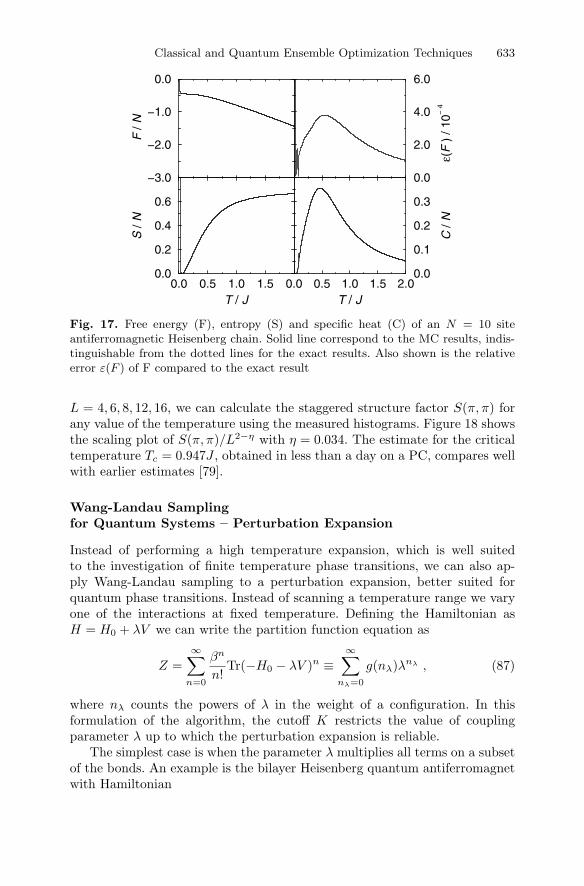
Classical and Quantum Ensemble Optimization Techniques 633
0.0 0.5 1.0 1.5T / J
0.0
0.2
0.4
0.6
S /
N
−3.0
−2.0
−1.0
0.0
F /
N
0.0 0.5 1.0 1.5 2.0T / J
0.0
0.1
0.2
0.3
C /
N
0.0
2.0
4.0
6.0
ε(F
) /
10−
4
Fig. 17. Free energy (F), entropy (S) and specific heat (C) of an N = 10 siteantiferromagnetic Heisenberg chain. Solid line correspond to the MC results, indis-tinguishable from the dotted lines for the exact results. Also shown is the relativeerror ε(F ) of F compared to the exact result
L = 4, 6, 8, 12, 16, we can calculate the staggered structure factor S(π, π) forany value of the temperature using the measured histograms. Figure 18 showsthe scaling plot of S(π, π)/L2−η with η = 0.034. The estimate for the criticaltemperature Tc = 0.947J , obtained in less than a day on a PC, compares wellwith earlier estimates [79].
Wang-Landau Samplingfor Quantum Systems – Perturbation Expansion
Instead of performing a high temperature expansion, which is well suitedto the investigation of finite temperature phase transitions, we can also ap-ply Wang-Landau sampling to a perturbation expansion, better suited forquantum phase transitions. Instead of scanning a temperature range we varyone of the interactions at fixed temperature. Defining the Hamiltonian asH = H0 + λV we can write the partition function equation as
Z =∞∑
n=0
βn
n!Tr(−H0 − λV )n ≡
∞∑
nλ=0
g(nλ)λnλ , (87)
where nλ counts the powers of λ in the weight of a configuration. In thisformulation of the algorithm, the cutoff K restricts the value of couplingparameter λ up to which the perturbation expansion is reliable.
The simplest case is when the parameter λ multiplies all terms on a subsetof the bonds. An example is the bilayer Heisenberg quantum antiferromagnetwith Hamiltonian

634 S. Trebst and M. Troyer
0.4 0.8 1.2 1.6 2.0
T / J
0.0
0.2
0.4
0.6
0.8
1.0
S(π
,π)
/ L 2
−η
0.0 1.0 2.0
T / J
0.0
0.5
1.0
C /
L3
L=12
L=8
L=6
L=4
L=16
Fig. 18. Scaling plot of the staggered structure factor of a cubic antiferromagnetas a function of temperature, obtained from simulations at a fixed temperature forvarious lattice sizes. The inset shows the specific heat as a function of temperature.The cutoff K = 500(L/4)3 restricts the accessible temperature range to T 0.4J
Hbilayer = J
2∑
l=1
∑
〈i,j〉Si,lSj,l + J ′
∑
〈i,j〉Si,1Sj,2 , (88)
where Si,l is the spin operator on site i in layer l. This model consists of twosquare lattices with coupling J between nearest neighbors inside each squarelattice layer, and a coupling J ′ between adjacent spins in different layers, andwe set λ = J/J ′. For such models the algorithm remains very simple, andagain only a few acceptance rates need to be changed in the code.
To normalize g(nλ) there are two options. If H0 can be solved exactly, g(0)can be determined directly. Otherwise, the normalization can be fixed usingthe high temperature expansion version of the algorithm to calculate Z(β) atany fixed value of λ. Even without normalization we can still obtain entropyand energy differences.
We consider as an example the quantum phase transition in the bilayerHeisenberg antiferromagnet. Its ground state changes from quantum disor-dered to Neel ordered as the ratio λ = J/J ′ of intra-plane (J) to inter-plane(J ′) coupling is increased [80]. From the histograms generated within one sim-ulation we can calculate the staggered structure factor S(π, π) of the systemat any value of λ. In Fig. 19 we show a scaling plot of S(π, π)/L2−z−η as afunction of λ. In short simulations, taking only a few days on a PC, we find thequantum critical point at λ = 0.396, which again compares well with earlierresults.

Classical and Quantum Ensemble Optimization Techniques 635
0.0 0.2 0.4 0.6 0.8 1.0J / J’
0.0
0.5
1.0
1.5
2.0
S(π
,π)
/ L 2
−z−
η
L=6
L=8
L=12
L=16
L=4
Fig. 19. Scaling plot of the staggered structure factor of a Heisenberg bilayer as afunction of the coupling ratio λ = J/J ′. Results are shown for various linear systemsizes L. The temperature was chosen βJ ′ = 2L, low enough to be in the scalingregime. The cutoff K = 8L3 was chosen large enough to cover the coupling rangeJ/J ′ 1. The dynamical critical exponent of this model is z = 1 and η = 0.034
Optimized Ensembles for Quantum Systems
As in classical Monte Carlo simulations it turns out that a flat histogram H(n)of the expansion orders n is not optimal, and again an optimized ensemblecan be derived.
6 Summary
In this chapter we have reviewed two recent developments in the field ofclassical and quantum Monte Carlo simulations. In the first part we havepresented a short review of extended ensemble techniques, including multi-canonical and parallel tempering simulations. Counter widespread assump-tions “flat-histogram” multicanonical ensembles, or parallel tempering withconstant, “flat” acceptance rates are not optimal. We have reviewed a recentlydeveloped iterative feedback algorithm to obtain an optimal multicanonicalensemble or an optimal choice of temperature set respectively that for a givenmodel will maximize equilibration. We have shown examples ranging fromclassical spin systems, over dense liquids to protein folding.
In the second part we have given a short introduction and review of mod-ern world line quantum Monte Carlo algorithms for quantum systems, whichare free of any time discretization errors. We have highlighted the fact that

636 S. Trebst and M. Troyer
the various world line representations map the quantum system to an effec-tive classical system, and shown how efficient sampling schemes developedfor classical simulations, such as histogram reweighting, parallel tempering,extended and optimized ensembles, can be applied also to quantum systems.
With examples ranging from quantum magnets to protein folding the en-semble optimization techniques have already been demonstrated to be usefulfor a wide range of models and scales, and will certainly help with the simu-lation of many other complex systems in the future.
References
1. F. Barahona (1982) On the computational complexity of Ising spin glass models.J. Phys. A 15, p. 3241
2. S. Cook (1971) The complexity of theorem-proving procedures. ConferenceRecord of Third Annual ACM Symposium on Theory of Computing, pp. 151–158
3. J. Kim and M. Troyer (1998) Low temperature behavior and crossovers of thesquare lattice quantum Heisenberg antiferromagnet. Phys. Rev. Lett. 80, p. 2705
4. M. Troyer and U.-J. Wiese (2005) Computational complexity and fundamentallimitations to fermionic quantum Monte Carlo simulations. Phys. Rev. Lett. 94,p. 170201
5. N. Metropolis, A. R. Rosenbluth, M. N. Rosenbluth, A. H. Teller, and E. Teller(1953) Equation of state calculations on fast computing machines. J. of Chem.Phys. 21, p. 1087
6. R. Swendsen and J.-S. Wang (1987) Nonuniversal critical dynamics in MonteCarlo simulations. Phys. Rev. Lett. 58, p. 86
7. U. Wolff (1989) Collective Monte Carlo updating for spin systems. Phys. Rev.Lett. 62, p. 361
8. O. Redner, J. Machta, and L. F. Chayes (1998) Graphical representations andcluster algorithms for critical points with fields. Phys. Rev. E 58, p. 2749
9. H. Evertz, H. Erkinger, and W. von der Linden (2002) New cluster method forthe Ising mode. In: Computer Simulations in Condensed Matter Physics, eds.D. Landau, S. P. Lewis, H.-B. Schuttler, vol. XIV, Springer, Berlin, p. 123
10. F. Alet, P. Dayal, A. Grzesik, A. Honecker, M. Korner, A. Lauchli, S. Man-mana, I. McCulloch, F. Michel, R. Noack, G. Schmid, U. Schollwock, F. Stockli,S. Todo, S. Trebst, M. Troyer, P. Werner, and S. Wessel (2005) The ALPSproject: open source software for strongly correlated systems. J. Phys. Soc.Jpn. Suppl. 74, p. 30
11. B. A. Berg and T. Neuhaus (1991) Multicanonical algorithms for first orderphase transitions. Phys. Lett. B 267, p. 249
12. B. A. Berg and T. Neuhaus (1992) Multicanonical ensemble: A new approachto simulate first-order phase transitions. Phys. Rev. Lett. 68, p. 9
13. F. Wang and D. P. Landau (2001) Efficient, multiple-range random walk algo-rithm to calculate the density of states. Phys. Rev. Lett. 86, p. 2050
14. F. Wang and D. P. Landau (2001) Determining the density of states for classicalstatistical models: A random walk algorithm to produce a flat histogram. Phys.Rev. E 64, p. 056101

Classical and Quantum Ensemble Optimization Techniques 637
15. C. Zhou and R. N. Bhatt (2005) Phys. Rev. E 72, p. 025701(R)16. H. K. Lee, Y. Okabe, and D. P. Landau (2006) Convergence and Refinement of
the Wang-Landau Algorithm. Comp. Phys. Comm. 175, p. 3617. P. Dayal, S. Trebst, S. Wessel, D. Wurtz, M. Troyer, S. Sabhapandit, and
S. N. Coppersmith (2004) Performance limitations of flat-histogram methods.Phys. Rev. Lett. 92, p. 097201
18. Y. Wu, M. Korner, L. Colonna-Romano, S. Trebst, H. Gould, J. Machta, andM. Troyer (2005) Overcoming the critical slowing down of flat-histogram MonteCarlo simulations: Cluster updates and optimized broad-histogram ensembles.Phys. Rev. E 72, p. 046704
19. S. Alder, S. Trebst, A. K. Hartmann, and M. Troyer (2004) Dynamics ofthe Wang-Landau algorithm and Complexity of rare events for the three-dimensional bimodal Ising spin glass. J. Stat. Mech. P07008
20. S. Trebst, D. A. Huse, and M. Troyer (2004) Optimizing the ensemble for equili-bration in broad-histogram Monte Carlo simulations. Phys. Rev. E 70, p. 046701
21. S. Trebst, E. Gull, and M. Troyer (2005) Optimized ensemble Monte Carlosimulations of dense Lennard-Jones fluids. J. Chem. Phys. 123, p. 204501
22. R. H. Swendsen and J. Wang (1986) Replica Monte Carlo Simulation of Spin-Glasses. Phys. Rev. Lett. 57, p. 2607
23. E. Marinari and G. Parisi (1992) Simulated tempering: A new Monte Carloscheme. Europhys. Lett. 19, p. 451
24. A. P. Lyubartsev, A. A. Martsinovski, S. V. Shevkunov, and P. N. Vorontsov-Velyaminov (1992) J. Chem. Phys. 96, p. 1776
25. K. Hukushima and Y. Nemoto (1996) Exchange Monte Carlo method and ap-plication to spin glass simulations. J. Phys. Soc. Jpn. 65, p. 1604
26. H. G. Katzgraber, S. Trebst, D. A. Huse, and M. Troyer (2006) J. Stat. Mechp. P03018
27. S. Trebst, M. Troyer, and U. H. E. Hansmann (2006) Optimized parallel tem-pering simulations of proteins. J. Chem. Phys. 124 p. 174903
28. J. C. McKnight, D. S. Doering, P. T. Matsudaira, and P. S. Kim (1996) Athermostable 35-residue subdomain within villin headpiece. J. Mol. Biol. 260,p. 126
29. Y. Duan and P. A. Kollman (1998) Pathways to a protein folding intermediateobserved in a 1-microsecond simulation in aqueous solution. Science 282, p. 740
30. B. Zagrovic, C. D. Snow, S. Khaliq, M. R. Shirts, and V. S. Pande (2002) Native-like mean structure in the unfolded ensemble of small proteins. J. Mol. Biol.323, p. 153
31. C.-Y. Liu, C.-K. Hu, and U. H. E. Hansmann (2003) Parallel tempering simu-lations of HP-36. Proteins: Struct., Funct., Genet. 52, p. 436
32. U. H. E. Hansmann (2004) Simulations of a small protein in a specifically de-signed generalized ensemble. Phys. Rev. E 70, p. 012902
33. M. J. Sippl, G. Nemethy, and H. A. Sheraga (1984) Intermolecular potentialsfrom crystal data. 6. Determination of empirical potentials for O-H...O=C hy-drogen bonds from packing configurations. J. Phys. Chem. 88, p. 6231
34. T. Ooi, M. Oobatake, G. Nemethy, and H. A. Scheraga (1987) Accessible surface-areas as a measure of the thermodynamic parameters of hydration of peptides.Proc. Natl. Acad. Sci. 84, p. 3086
35. M. Troyer, S. Wessel, and F. Alet (2003) Flat histogram methods for quan-tum systems: algorithms to overcome tunneling problems and calculate the freeenergy. Phys. Rev. Lett. 90, p. 120201

638 S. Trebst and M. Troyer
36. M. Troyer, F. Alet, and S. Wessel (2004) Histogram methods for quantum sys-tems: from reweighting to Wang-Landau sampling. Braz. J. of Physics 34,p. 377
37. R. Feynman (1953) Atomic theory of liquid helium near absolute zero. Phys.Rev. 91, p. 1301
38. H. Trotter (1959) On the product of semi-groups of operators. Proc. Am. Math.Soc. 10, p. 545
39. M. Suzuki (1976) Relationship between d-dimensional quantal spin systems and(d+1)-dimensional Ising systems – Equivalence, Critical Exponents and Sys-tematic Approximants of the Partition Function and Spin Correlations. Prog.Theor. Phys. 56, p. 1454
40. N. V. Prokofev, B. V. Svistunov, and I. S. Tupitsyn (1998) Exact, complete,and universal continuous-time worldline Monte Carlo approach to the statisticsof discrete quantum systems. JETP 87, p. 310
41. A. Sandvik and J. Kurkijarvi (1991) Quantum Monte Carlo simulation methodfor spin systems. Phys. Rev. B 43, p. 5950
42. D. Handscomb (1962) The Monte Carlo method in quantum statistical mechan-ics. Proc. Cambridge Philos. Soc. 58, p. 594
43. S. Sachdev, P. Werner, and M. Troyer (2004) Universal conductance of quantumwires near the superconductor-metal quantum transition. Phys. Rev. Lett. 92,p. 237003
44. P. Werner, K. Volker, M. Troyer, and S. Chakravarty (2005) Phase diagram andcritical exponents of a dissipative Ising spin chain in a transverse magnetic field.Phys. Rev. Lett. 94, p. 047201
45. E. L. Pollock and D. M. Ceperley (1987) Path-integral computation of superfluiddensities. Phys. Rev. B 36, p. 8343
46. M. Jarrell and J. Gubernatis (1996) Bayesian inference and the analytic contin-uation of imaginary time Monte Carlo data. Physics Reports 269, p. 133
47. W. von der Linden (1995) Maximum-entropy data analysis. Applied Physics A60, p. 155
48. K. S. D. Beach (2004) Identifying the maximum entropy method as a speciallimit of stochastic analytic continuation. cond-mat/0403055
49. M. Suzuki, S. Miyashita, and A. Kuroda (1977) Monte Carlo simulation ofquantum spin systems. I. Prog. Theor. Phys. 58, p. 1377
50. N. V. Prokofev, B. V. Svistunov, and I. S. Tupitsyn (1996) Exact quantumMonte Carlo process for the statistics of discrete systems. JETP Lett. 64, p. 911
51. M. S. Makivic and H. Q. Ding (1991) Two-dimensional spin-1/2 Heisenbergantiferromagnet: A quantum Monte Carlo study. Phys. Rev. B 43, p. 3562
52. H. G. Evertz, G. Lana, and M. Marcu (1993) Cluster algorithm for vertex mod-els. Phys. Rev. Lett. 70, p. 875
53. B. Beard and U. Wiese (1996) Simulations of discrete quantum systems in con-tinuous Euclidean time. Phys. Rev. Lett. 77, p. 5130
54. H. G. Evertz (2003) The loop algorithm. Adv. in Physics 52, p. 155. N. Kawashima and K. Harada (2004) Recent developments of world-line Monte
Carlo methods. J. Phys. Soc. Jpn. 73, p. 137956. N. Kawashima and J. Gubernatis (1994) Loop algorithms for Monte Carlo sim-
ulations of quantum spin systems. Phys. Rev. Lett. 73, p. 129557. N. Kawashima and J. Gubernatis (1995) Generalization of the Fortuin-
Kasteleyn transformation and its application to quantum spin simulations. J.Stat. Phys. 80, p. 169

Classical and Quantum Ensemble Optimization Techniques 639
58. K. Harada, M. Troyer and N. Kawashima (1998) The two-dimensional spin-1quantum Heisenberg antiferromagnet at finite temperatures. J. Phys. Soc. Jpn.67, p. 1130
59. S. Todo and K. Kato (2001) Cluster algorithms for general-S quantum spinsystems. Phys. Rev. Lett. 87, p. 047203
60. N. Kawashima (1996) Cluster algorithms for anisotropic quantum spin models.J. Stat. Phys. 82, p. 131
61. A. Sandvik (1999) Stochastic series expansion method with operator-loop up-date. Phys. Rev. B 59, p. R14157
62. A. Dorneich and M. Troyer (2001) Accessing the dynamics of large many-particlesystems using the stochastic series expansion. Phys. Rev. E 64, p. 066701
63. O. Syljuasen and A. W. Sandvik (2002) Quantum Monte Carlo with directedloops. Phys. Rev. E 66, p. 046701
64. U.-J. Wiese and H.-P. Ying (1992) Blockspin cluster algorithms for quantumspin systems. Phys. Lett. A 168, p. 143
65. B. Frischmuth, B. Ammon, and M. Troyer (1996) Susceptibility and low-temperature thermodynamics of spin-1/2 Heisenberg ladders. Phys. Rev. B54, p. R3714
66. M. Greven, R. J. Birgeneau, and U. J. Wiese (1996) Monte Carlo study ofcorrelations in quantum spin ladders. Phys. Rev. Lett. 77, p. 1865
67. M. Troyer, M. Imada, and K. Ueda (1997) Critical exponents of the quantumphase transition in a planar antiferromagnet. J. Phys. Soc. Jpn. 66, p. 2957
68. B. B. Beard, R. J. Birgeneau, M. Greven, and U.-J. Wiese (1998) Square-latticeHeisenberg antiferromagnet at very large correlation lengths. Phys. Rev. Lett.80, p. 1742
69. C. Yasuda, S. Todo, K. Hukushima, F. Alet, M. Keller, M. Troyer, andH. Takayama (2005) Neel temperature of quasi-low-dimensional Heisenberg an-tiferromagnets. Phys. Rev. Lett. 94, p. 217201
70. D. C. Johnston, M. Troyer, S. Miyahara, D. Lidsky, K. Ueda, M. Azuma,Z. Hiroi, M. Takano, M. Isobe, Y. Ueda, M. A. Korotin, V. I. Anisimov, A. V.Mahajan, and L. L. Miller (2000) Magnetic susceptibilities of spin-1/2 anti-ferromagnetic Heisenberg ladders and applications to ladder oxide compounds.cond-mat/0001147
71. D. C. Johnston, R. K. Kremer, M. Troyer, X. Wang, A. Klumper, S. L. Budko,A. F. Panchula, and P. C. Canfield (2000) Thermodynamics of spin S=1/2antiferromagnetic uniform and alternating-exchange Heisenberg chains. Phys.Rev. B 61, p. 9558
72. R. Melzi, P. Carretta, A. Lascialfari, M. Mambrini, M. Troyer, P. Millet, andF. Mila (1999) Li2VO(Si,Ge)O4, a prototype of a two-dimensional frustratedquantum Heisenberg antiferromagnet. Phys. Rev. Lett. 85, p. 1318
73. M. A. Korotin, I. S. Elfimov, V. I. Anisimov, M. Troyer, and D. I. Khomskii(1998) Exchange interactions and magnetic properties of the layered vanadatesCaV2O5, MgV2O5, CaV3O7, and CaV4O9. Phys. Rev. Lett. 83, p. 1387
74. F. Woodward, A. Albrecht, C. Wynn, C. P. Landee, and M. Turnbull (2002)Two-dimensional S= 1/2 Heisenberg antiferromagnets: Synthesis, structure, andmagnetic properties. Phys. Rev. B 65, p. 144412
75. G. Schmid, S. Todo, M. Troyer, and A. Dorneich (2002) Finite-temperaturephase diagram of hard-core bosons in two dimensions. Phys. Rev. Lett. 88,p. 167208

640 S. Trebst and M. Troyer
76. O. Nohadani, S. Wessel, B. Normand, and S. Haas (2004) Universal scaling atfield-induced magnetic phase transitions. Phys. Rev. B 69, p. 220402
77. A. Ferrenberg and R. Swendsen (1988) New Monte Carlo technique for studyingphase transitions. Phys. Rev. Lett. 61, p. 2635
78. A. Ferrenberg and R. Swendsen (1989) Optimized Monte Carlo data analysis.Phys. Rev. Lett. 63, p. 1195
79. A. Sandvik (1998) Critical temperature and the transition from quantum toclassical order parameter fluctuations in the three-dimensional Heisenberg an-tiferromagnet. Phys. Rev. Lett. 80, p. 5196
80. A. Sandvik (1994) Order-disorder transition in a two-layer quantum antiferro-magnet. Phys. Rev. Lett. 72, p. 2777