Ensemble Forecasting - UMCP Chaos Weather Project€¦ · Each ensemble member evolution is given...

Ensemble Forecasting

Yuejian Zhu Ensemble team leader

Environmental Modeling Center NCEP/NWS/NOAA

Acknowledgements: EMC Ensemble team staffs

January 28 2013

Uncertainties & disagreements

Ensemble forecast is widely used in daily weather forecast

December 2012 was 20 anniversary of both NCEP and ECMWF global ensemble

operational implementation

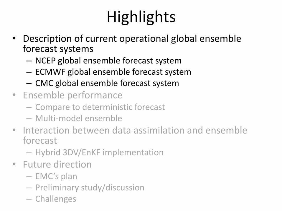
Highlights • Description of current operational global ensemble

forecast systems – NCEP global ensemble forecast system – ECMWF global ensemble forecast system – CMC global ensemble forecast system

• Ensemble performance – Compare to deterministic forecast – Multi-model ensemble

• Interaction between data assimilation and ensemble forecast – Hybrid 3DV/EnKF implementation

• Future direction – EMC’s plan – Preliminary study/discussion – Challenges

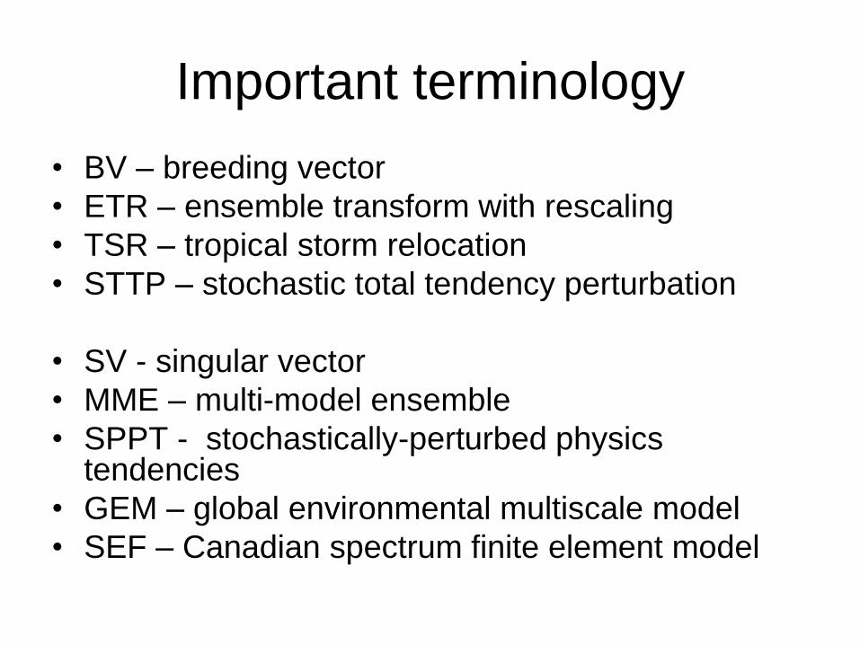
Important terminology

• BV – breeding vector

• ETR – ensemble transform with rescaling

• TSR – tropical storm relocation

• STTP – stochastic total tendency perturbation

• SV - singular vector

• MME – multi-model ensemble

• SPPT - stochastically-perturbed physics tendencies

• GEM – global environmental multiscale model

• SEF – Canadian spectrum finite element model

Each ensemble member evolution is given by integrating the following equation

where ej(0) is the initial condition, Pj(ej,t) represents the model tendency component due to parameterized physical processes (model uncertainty), dPj(ej,t) represents random model errors (e.g. due to parameterized physical processes or sub-grid scale processes – stochastic perturbation) and Aj(ej,t) is the remaining tendency component (different physical parameterization or multi-model).

Reference:

Buizza, R., P. L. Houtekamer, Z. Toth, G. Pellerin, M. Wei, Y. Zhu, 2005:

"A Comparison of the ECMWF, MSC, and NCEP Global Ensemble Prediction Systems“ Monthly Weather Review, Vol. 133, 1076-1097

T

t

jjjjjjjj dtteAtedPtePdeeTe0

0 )],(),(),([)0()0()(

Description of the ECMWF, MSC and NCEP systems

Operation: ECMWF-1992; NCEP-1992; MSC-1998

Initial uncertainty Model uncertainty

Initial

uncertainty

TS

relocation

Model

uncertainty

Resolution Forecast

length

Ensemble

members

Daily

frequency

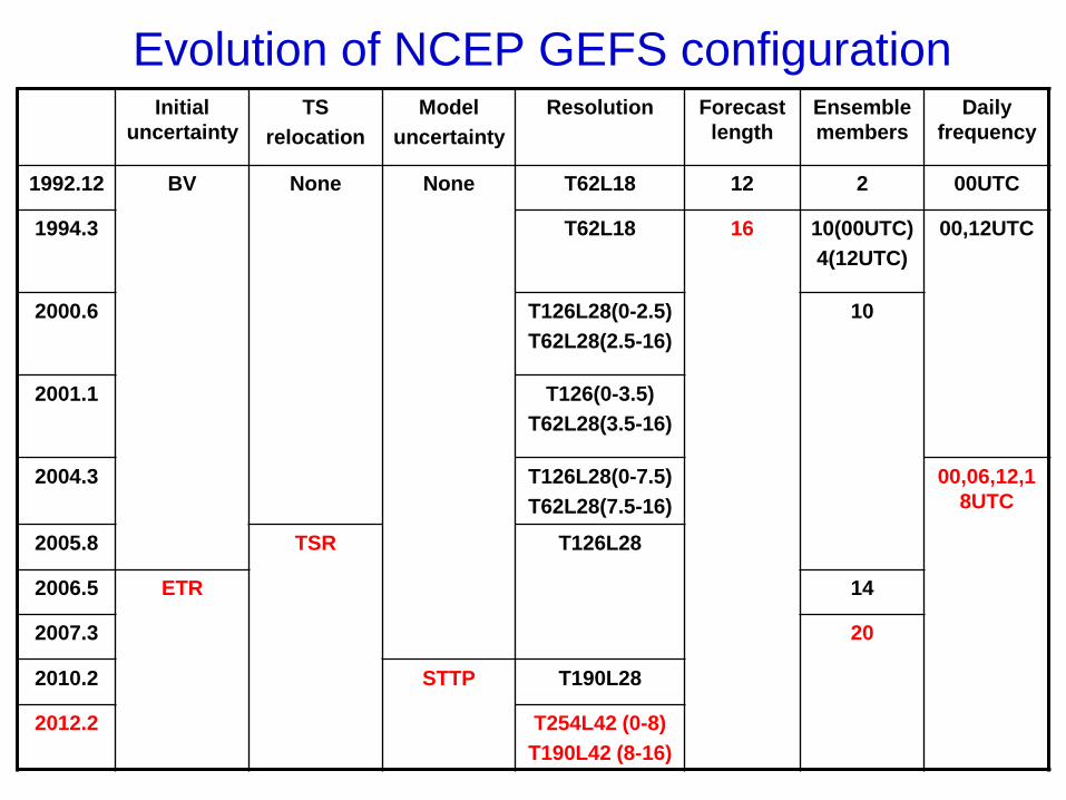
1992.12 BV None None T62L18 12 2 00UTC

1994.3 T62L18 16 10(00UTC)

4(12UTC)

00,12UTC

2000.6 T126L28(0-2.5)

T62L28(2.5-16)

10

2001.1 T126(0-3.5)

T62L28(3.5-16)

2004.3 T126L28(0-7.5)

T62L28(7.5-16)

00,06,12,1

8UTC

2005.8 TSR T126L28

2006.5 ETR 14

2007.3 20

2010.2 STTP T190L28

2012.2 T254L42 (0-8)

T190L42 (8-16)

Evolution of NCEP GEFS configuration

Estimating and Sampling Initial Errors: The Breeding Method - 1992

• DATA ASSIM: Growing errors due to cycling through NWP forecasts

• BREEDING: - Simulate effect of obs by rescaling nonlinear perturbations

– Sample subspace of most rapidly growing analysis errors

• Extension of linear concept of Lyapunov Vectors into nonlinear environment

• Fastest growing nonlinear perturbations

• Not optimized for future growth –

– Norm independent

– Is non-modal behavior important?

Courtesy of Zoltan Toth

References

1. Toth and Kalnay: 1993 BAMS

2. Tracton and Kalnay: 1993 WAF

3. Toth and Kalnay: 1997 MWR

P1

N1

P2

N2

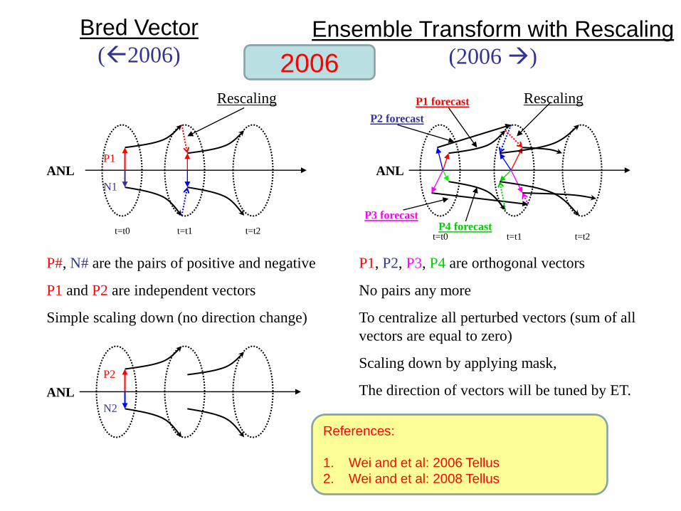
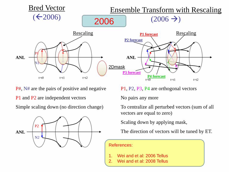
P#, N# are the pairs of positive and negative

P1 and P2 are independent vectors

Simple scaling down (no direction change)

Ensemble Transform with Rescaling

(2006 )

P1, P2, P3, P4 are orthogonal vectors

No pairs any more

To centralize all perturbed vectors (sum of all

vectors are equal to zero)

Scaling down by applying mask,

The direction of vectors will be tuned by ET.

Rescaling

ANL

ANL ANL

Bred Vector

(2006)

P1 forecast

P4 forecast P3 forecast

P2 forecast

t=t1 t=t0 t=t0

t=t2 t=t2 t=t1

Rescaling

2006

References:

1. Wei and et al: 2006 Tellus


P1

N1

P2

N2

P#, N# are the pairs of positive and negative

P1 and P2 are independent vectors

Simple scaling down (no direction change)

Ensemble Transform with Rescaling

(2006 )

P1, P2, P3, P4 are orthogonal vectors

No pairs any more

To centralize all perturbed vectors (sum of all

vectors are equal to zero)

Scaling down by applying mask,

The direction of vectors will be tuned by ET.

Rescaling

ANL

ANL ANL

Bred Vector

(2006)

P1 forecast

P4 forecast P3 forecast

P2 forecast

t=t1 t=t0 t=t0

t=t2 t=t2 t=t1

Rescaling

2006

References:



2Dmask

T00Z

10m

T06Z

10m

T18Z

10m

T12Z

10m

24hrs

24hrs

24hrs

24hrs

Re-scaling

Re-scaling

Re-scaling

Re-scaling

Up to 16-d

Up to 16-d

Up to 16-d

Up to 16-d

T00Z

40m

6hrs

T06Z

40m

T12Z

40m

T18Z

40m

Up to 16-d

Up to 16-d

Up to 16-d

Up to 16-d

Re-scaling

Re-scaling

Re-scaling

Re-scaling

24-hour breeding cycle

2004

6-hour breeding cycle

2004

Next T00Z

2004

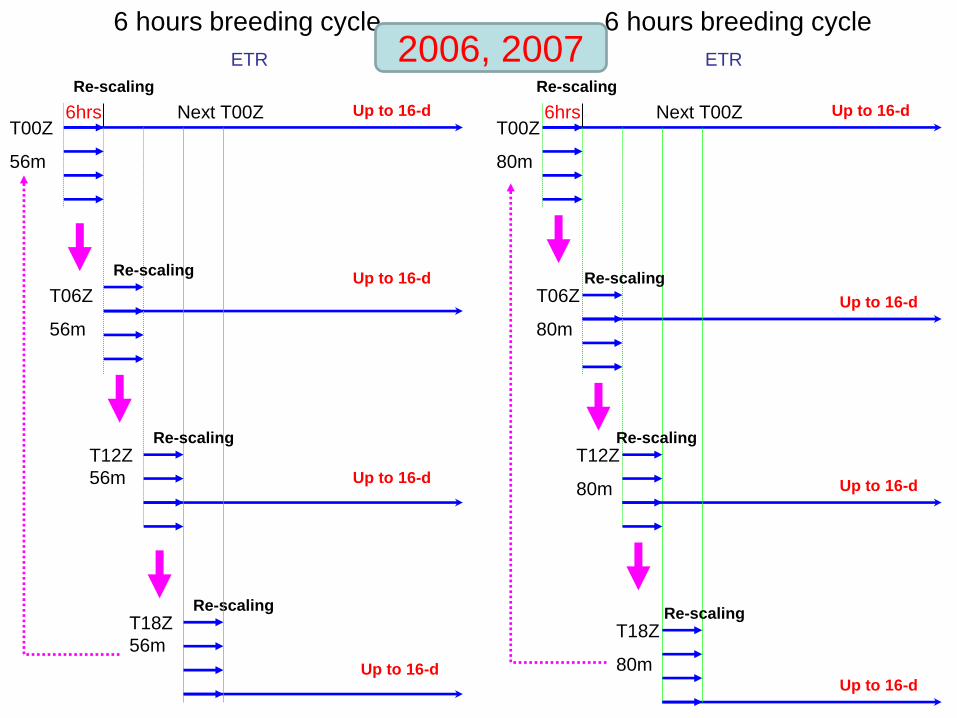
T00Z

56m

T06Z

56m

T18Z

56m

T12Z

56m

6hrs Next T00Z

Re-scaling

Re-scaling

Re-scaling

Up to 16-d

Up to 16-d

Up to 16-d

Up to 16-d

T00Z

80m

6hrs

T06Z

80m

T12Z

80m

T18Z

80m

Up to 16-d

Up to 16-d

Up to 16-d

Up to 16-d

Re-scaling

Re-scaling

Re-scaling

Re-scaling

6 hours breeding cycle

ETR

6 hours breeding cycle

ETR

Next T00Z

Re-scaling

2006, 2007

How do we tune ETR initial perturbations ?

500hPa

Surface

Top

20% more

same

same

Current operation Future

Rescaling mask and factors

Linear

500hPa NH

850hPa NH

1000hPa NH

Reference mask

1.0 factor

1.2 factor

Schematic of tuning initial perturbations

2012

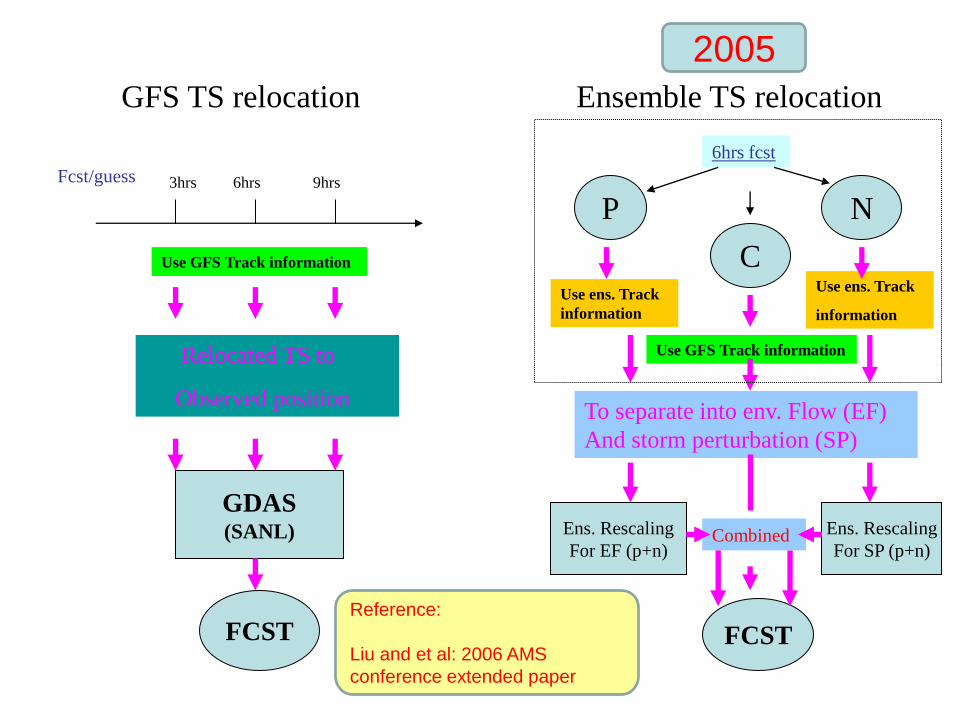
Fcst/guess 3hrs 9hrs 6hrs

Relocated TS to

Observed position

GDAS (SANL)

FCST

GFS TS relocation

P

C

N

6hrs fcst

Use ens. Track

information

Use GFS Track information

Use GFS Track information

Use ens. Track

information

To separate into env. Flow (EF)

And storm perturbation (SP)

FCST

Ensemble TS relocation

Ens. Rescaling

For SP (p+n)

Ens. Rescaling

For EF (p+n) Combined

2005

Reference:

Liu and et al: 2006 AMS

conference extended paper

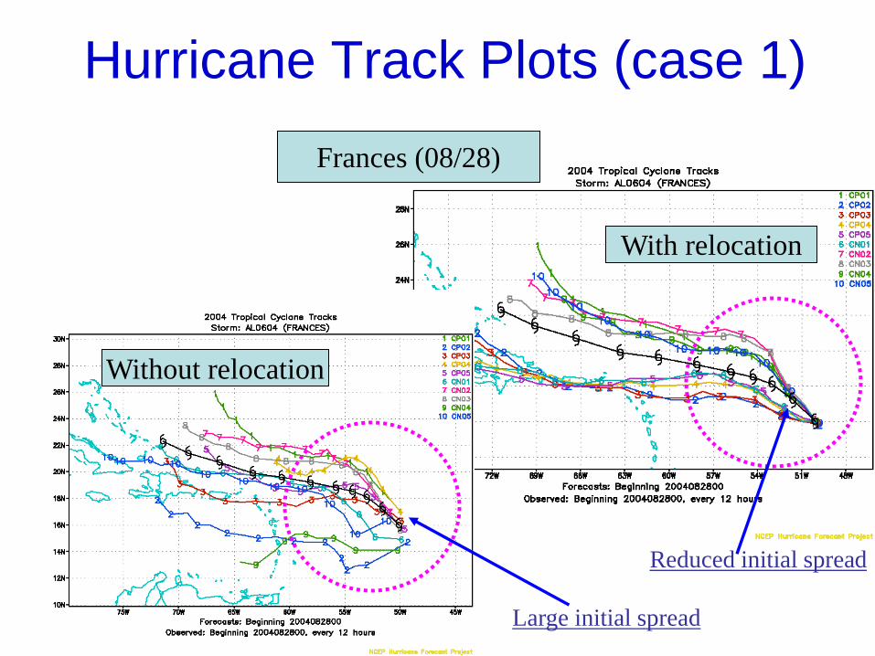
Hurricane Track Plots (case 1)

Frances (08/28)

Without relocation

With relocation

Large initial spread

Reduced initial spread

Hurricane Tracks Plots (case 2)

Ivan (09/14)

Without relocation

With relocation

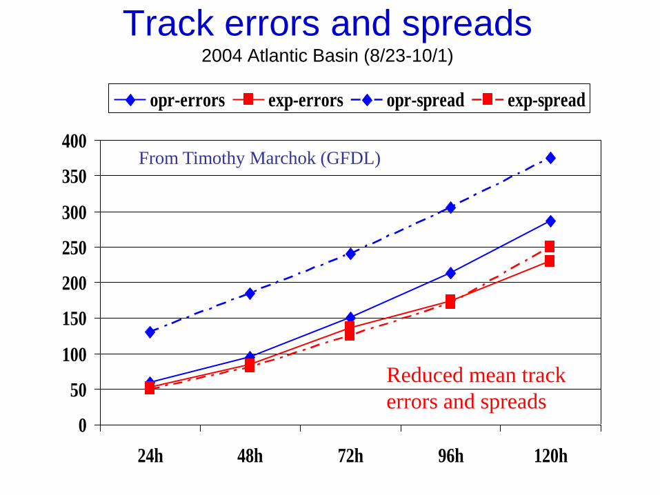
Track errors and spreads 2004 Atlantic Basin (8/23-10/1)

0

50

100

150

200

250

300

350

400

24h 48h 72h 96h 120h

opr-errors exp-errors opr-spread exp-spread

From Timothy Marchok (GFDL)

Reduced mean track

errors and spreads

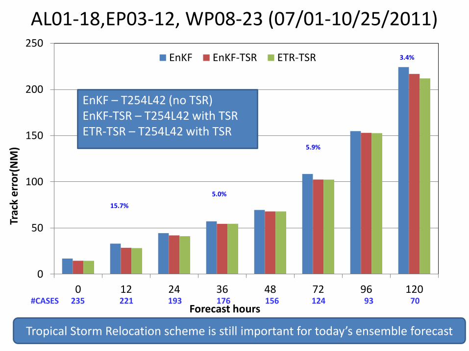
AL01-18,EP03-12, WP08-23 (07/01-10/25/2011)

0

50

100

150

200

250

0 12 24 36 48 72 96 120

EnKF EnKF-TSR ETR-TSR

EnKF – T254L42 (no TSR) EnKF-TSR – T254L42 with TSR ETR-TSR – T254L42 with TSR

15.7%

5.0%

5.9%

3.4%

Trac

k e

rro

r(N

M)

#CASES 235 221 193 176 156 124 93 70 Forecast hours

Tropical Storm Relocation scheme is still important for today’s ensemble forecast

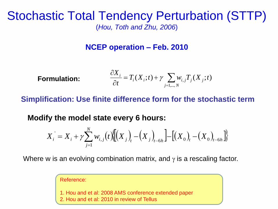
Stochastic Total Tendency Perturbation (STTP) (Hou, Toth and Zhu, 2006)

NCEP operation – Feb. 2010

htthtjtj

N

j

jiii XXXXtwXX6006

1

,

'

Simplification: Use finite difference form for the stochastic term

Modify the model state every 6 hours:

Where w is an evolving combination matrix, and is a rescaling factor.

);();(,...,1

, tXTwtXTt

Xjj

Nj

jiiii

Formulation:

Reference:

1. Hou and et al: 2008 AMS conference extended paper

2. Hou and et al: 2010 in review of Tellus

STTP Scheme Application Generation of Stochastic Combination Coefficients: • Matrix Notation (N forecasts at M points)

S (t) = P(t) W(t)

MxN MxN NxN

• As P is quasi orthogonal, an orthonormal matrix W ensures orthogonality for S.

• Generation of W matrix: (Methodology and software provided by James Purser).

– a) Start with a random but orthonormalized matrix W(t=0);

– b) W(t)=W(t-1) R0 R1(t)

• R0, R(t) represent random but slight rotation in N-Dimensional space

Random walk (R1) superimposed on a periodic

Function (R0)

wij(t) for i=14, and j=1,14

Experiments for 2009 Operational Implementation

T126L28 vs. T190L28 resolution, Nov. 2007 Cases

SPS works with both resolutions

--- T126L28

--- T126L28 + SP

--- T190L28

--- T190L28 + SP

CRPSS ROC

Random Model Error – Stochastic Schemes

• Stochastically-perturbed physics tendencies (SPPT) – operational

ECMWF scheme.

• Stochastic total tendency perturbation (STTP) – operational NCEP

scheme

• Vorticity confinement (VC) – under development at UKMet and

ECMWF

• Stochastically-perturbed boundary-layer humidity (SHUM)

• Perturbed convective trigger on SAS

– Testing on HWRF ensemble and global system

• Questions and issues

– Will these schemes help to increase ensemble spread?

– Will these schemes help to reduce missing forecast for extreme

weather events?

– What is the future of physical parameterizations?

• Deterministic or probabilistic?

Unperturbed Analysis - 4D-VAR (TL1279L91) EDA-based perturbation - the difference between the perturbed (perturb all obs and sea-surface T and use SPPT to simulate random model error) and unperturbed first-guesses (TL399L91) SV-based perturbation - initial singular vectors (T42L62)

EDA1

EDA2

EDA10 …

…

SV1 SV2 SV3 SV4 SV5

mem1

mem3 mem2

+

……

……

mem50

Initial Condition = Unperturbed Analysis + EDA-based perturbation + SV-based perturbation

SV6 SV7 SV8 SV9

SV10

+

Current ECMWF ensemble configuration

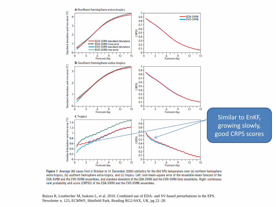
Buizza R, Leutbecher M, Isaksen L, et al. 2010. Combined use of EDA- and SV-based perturbations in the EPS.

Newsletter n. 123, ECMWF, Shinfield Park, Reading RG2-9AX, UK, pg 22–28.

Similar to EnKF, growing slowly,

good CRPS scores

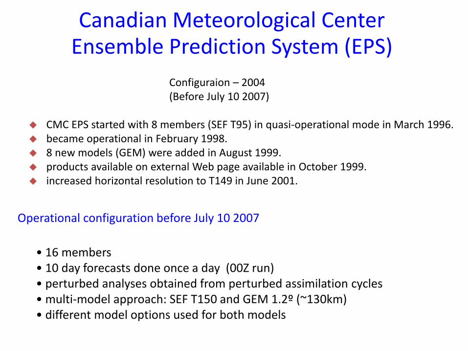
• 16 members • 10 day forecasts done once a day (00Z run) • perturbed analyses obtained from perturbed assimilation cycles • multi-model approach: SEF T150 and GEM 1.2º (~130km) • different model options used for both models

Canadian Meteorological Center Ensemble Prediction System (EPS)

Configuraion – 2004 (Before July 10 2007)

CMC EPS started with 8 members (SEF T95) in quasi-operational mode in March 1996. became operational in February 1998. 8 new models (GEM) were added in August 1999. products available on external Web page available in October 1999. increased horizontal resolution to T149 in June 2001.

Operational configuration before July 10 2007

perturbed trial fields perturbed observations

perturbed analyses

doubling of the number of analyses

models

8 models each producing A data assimilation cycle

16 forecast cycles • 8 SEF - T149 or ~150 km • 8 GEM - 1.2° or ~135 km • 10 days at 00 UTC

16 members

Canadian Meteorological Center Ensemble Prediction System (EPS)

Configuration - 2004

SEF (T149) Add ops Convection/Radiation GWD GWD Orography Number Time level analysis version of levels 1 yes Kuo/ Garand Strong High altitude 0.3 23 3 2 no Manabe/ Sasamori Strong Low altitude 0.3 41 3 3 no Kuo/ Garand Weak Low altitude Mean 23 3 4 yes Manabe/ Sasamori Weak High altitude Mean 41 3 5 yes Manabe/ Sasamori Strong Low altitude Mean 23 2 6 no Kuo/ Garand Strong High altitude Mean 41 2 7 no Manabe/ Sasamori Weak High altitude 0.3 23 2 8 yes Kuo/ Garand Weak Low altitude 0.3 41 2 control mean Kuo/ Garand Mean Low altitude 0.15 41 3 GEM (1.20) Add ops Deep Shallow Soil Sponge Number Coriolis analysis convection convection moisture of levels 9 no Kuosym new Less 20% global 28 Implicit 10 yes RAS old Less 20% equatorial 28 Implicit 11 yes RAS old Less 20% global 28 Implicit 12 no Kuosym old More 20% global 28 Implicit 13 no Kuosym new More 20% global 28 Implicit 14 yes Kuosym new Less 20% global 28 Implicit 15 yes Kuosym old Less 20% global 28 Implicit 16 no OldKuo new More 20% global 28 Implicit

Combination of model perturbations (2004)

P. Houtekamer, ARMA

CMC’s Multi-model EPS for the assimilation (current-GEM) # Deep convection Surface scheme Mixing length Vertical mixing parameter

1

2

3

4

5

Kain & Fritsch

Oldkuo

Relaxed Arakawa Schubert

Kuo Symétrique

Oldkuo

ISBA

ISBA

force-restore

force-restore

force-restore

Bougeault

Blackadar

Bougeault

Blackadar

Bougeault

1.0

0.85

0.85

1.0

1.0

6

7

8

9

10

Kain & Fritsch

Kuo Symétrique


Kain & Fritsch

Oldkuo

force-restore

ISBA

ISBA

ISBA

ISBA

Blackadar

Bougeault

Blackadar

Blackadar

Bougeault

0.85

0.85

1.0

0.85

1.0

11

12

13

14

15


Kuo Symétrique

Oldkuo

Kain & Fritsch

Kuo Symétrique

force-restore

force-restore

force-restore

force-restore

ISBA

Blackadar

Bougeault

Blackadar

Bougeault

Blackadar

1.0

0.85

0.85

1.0

1.0

16

17

18

19

20


Kuo Symmetric

Kain & Fritsch

Oldkuo


ISBA

force-restore

ISBA

ISBA

force-restore

Bougeault

Bougeault

Blackadar

Bougeault

Blackadar

0.85

1.0

0.85

0.85

1.0

21

22

23

24


Oldkuo

Kain & Fritsch

Kuo Symétrique

ISBA

force-restore

force-restore

ISBA

Blackadar

Bougeault

Blackadar

Bougeault

0.85

1.0

1.0

0.85

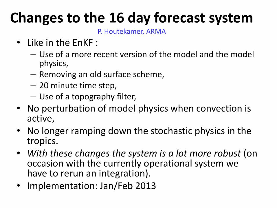
Changes to the 16 day forecast system P. Houtekamer, ARMA

• Like in the EnKF : – Use of a more recent version of the model and the model

physics, – Removing an old surface scheme, – 20 minute time step, – Use of a topography filter,

• No perturbation of model physics when convection is active,

• No longer ramping down the stochastic physics in the tropics.

• With these changes the system is a lot more robust (on occasion with the currently operational system we have to rerun an integration).

• Implementation: Jan/Feb 2013

NH Anomaly Correlation for 500hPa Height Period: January 1st – December 31st 2012

0

0.1

0.2

0.3

0.4

0.5

0.6

0.7

0.8

0.9

1

1 2 3 4 5 6 7 8 9 10 11 12 13 14 15

An

om

aly

Co

rre

lati

on

Forecast (days)

GFS GEFS NAEFS Ensemble mean

Skillful forecast

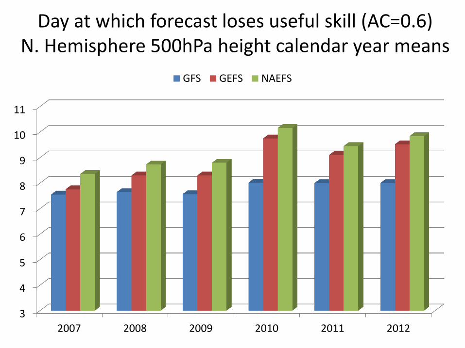
Day at which forecast loses useful skill (AC=0.6) N. Hemisphere 500hPa height calendar year means

3

4

5

6

7

8

9

10

11

2007 2008 2009 2010 2011 2012

GFS GEFS NAEFS

Continuous Ranked Probability Skill Scores

5 days forecast

10 days forecast

0

50

100

150

200

250

300

350

400

450

0 12 24 36 48 72 96 120 144 168

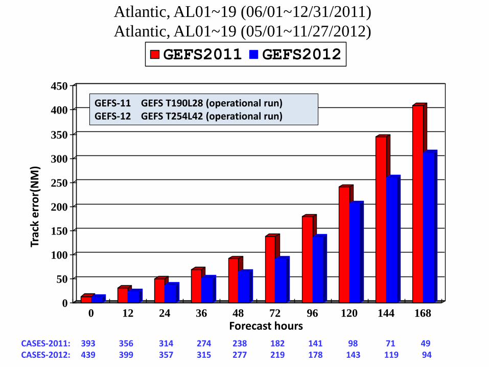
GEFS2011 GEFS2012

Trac

k e

rro

r(N

M)

Forecast hours

CASES-2011: 393 356 314 274 238 182 141 98 71 49 CASES-2012: 439 399 357 315 277 219 178 143 119 94

Atlantic, AL01~19 (06/01~12/31/2011)

Atlantic, AL01~19 (05/01~11/27/2012)

GEFS-11 GEFS T190L28 (operational run) GEFS-12 GEFS T254L42 (operational run)

0

50

100

150

200

250

1 2 3 4 5 6 7 8

GFS GEFS EC_det EC_ens

ECMWF made better forecast

Track Forecast Error for Atlantic 2012 Season

FCST HOURS 0 12 24 36 48 72 96 120 Cases 170 151 137 123 110 90 73 57

GFS – NCEP deterministic forecast GEFS – NCEP ensemble forecast EC_det – ECWMF deterministic forecast EC_ens – ECMWF ensemble forecast

NCEP made better forecast

Interactions between DA and EPS

Ideally, EPS and DA systems should be consistent for

best performance of both.

DA provides best estimates of initial uncertainties, i.e. analysis

error covariance for EPS.

EPS produces accurate flow dependent forecast (background)

covariance for DA.

)( aP

DA EPS f

P

Best analysis error variances

Accurate forecast error covariance

EnKF member update

member 2 analysis

high res forecast

GSI Hybrid Ens/Var

high res analysis

member 1 analysis

member 2 forecast

member 1 forecast

recenter an

alysis ense

mb

le

NCEP Dual-Res Coupled Hybrid DA System

member 3 forecast

member 3 analysis

Previous Cycle Current Update Cycle

T25

4L6

4

T57

4L6

4

Generate new ensemble perturbations given the

latest set of observations and first-guess ensemble

Ensemble contribution to background error

covariance Replace the EnKF

ensemble mean analysis

Courtesy of Daryl Kleist

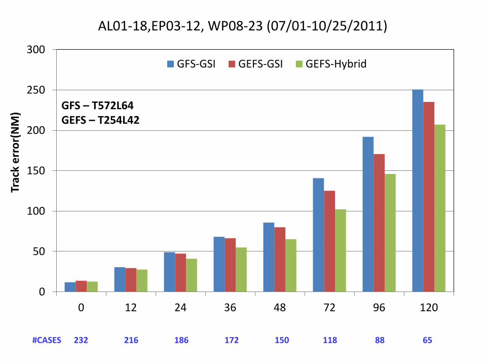
AL01-18,EP03-12, WP08-23 (07/01-10/25/2011)

0

50

100

150

200

250

300

0 12 24 36 48 72 96 120

GFS-GSI GEFS-GSI GEFS-Hybrid

Trac

k e

rro

r(N

M)

#CASES 232 216 186 172 150 118 88 65

GFS – T572L64 GEFS – T254L42

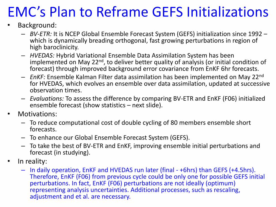
EMC’s Plan to Reframe GEFS Initializations • Background:

– BV-ETR: It is NCEP Global Ensemble Forecast System (GEFS) initialization since 1992 – which is dynamically breading orthogonal, fast growing perturbations in region of high baroclinicity.

– HVEDAS: Hybrid Variational Ensemble Data Assimilation System has been implemented on May 22nd, to deliver better quality of analysis (or initial condition of forecast) through improved background error covariance from EnKF 6hr forecasts.

– EnKF: Ensemble Kalman Filter data assimilation has been implemented on May 22nd for HVEDAS, which evolves an ensemble over data assimilation, updated at successive observation times.

– Evaluations: To assess the difference by comparing BV-ETR and EnKF (F06) initialized ensemble forecast (show statistics – next slide).

• Motivations: – To reduce computational cost of double cycling of 80 members ensemble short

forecasts. – To enhance our Global Ensemble Forecast System (GEFS). – To take the best of BV-ETR and EnKF, improving ensemble initial perturbations and

forecast (in studying).

• In reality: – In daily operation, EnKF and HVEDAS run later (final - +6hrs) than GEFS (+4.5hrs).

Therefore, EnKF (F06) from previous cycle could be only one for possible GEFS initial perturbations. In fact, EnKF (F06) perturbations are not ideally (optimum) representing analysis uncertainties. Additional processes, such as rescaling, adjustment and et al. are necessary.

Comparison of ETR .vs EnKF (f06) initialized ensemble forecasts

Summer 2011 Winter 11/12 Summer 2012

NH 500hPa Z PAC NH 500hPa Z PAC NH 500hPa Z PAC

SH 500hPa Z PAC

Summer 2012

Summary of comparison: (Three seasons – Summer 2011, Winter

2011/2012 and Summer 2012)

1. For Northern Hemisphere ensemble mean and probabilistic forecasts – they are very similar to each other; the differences are insignificant mostly. EnKF has a little better probabilistic forecast for very short lead time due to larger spread.

2. For Southern Hemisphere mean and probabilistic forecast – ETR is better than EnKF, especially for the two summer seasons. EnkF is over dispersion for SH in generally.

3. Tropical Storm track forecast, ETR and EnKF have similar forecast errors and ensemble spread for two summer seasons. The differences are insignificant.

4. For summer 2012, ETR is better than EnKF’s performance over all.

TS track forecast errors – Summer 2011

SH 500hPa Z RMS and Spread 0

50

100

150

200

250

0 12 24 36 48 72 96 120

EnKF EnKF_sETR ETR_s

Solid – errors Dash - spread

Solid black – EnKF RMSE Dash black – EnKF spread

18Z 00Z

EnKF06

EnKF 6hr fcst

00Z 18Z

3DETR

ETR 6 hr fcst

Apply ET and 3D mask

3D mask is generated from accumulated EnKF

analysis variance. In general, it masks out very

fast growing and saturated modes.

ET is making initial perts orthogonally.

Advantage:

1. Selective potential growing mode;

2. All perturbations are orthogonal;

3. Continuation of vector (member) from cycle to

cycle.

Artificial inflation and centralization

EnKF update with observations, perts will

be reduced usually, inflation is need

Perturbations are decayed for first 3-9

hours because most of inflated

perturbations are non-growing, white noise

Schematic diagram of 00Z initial perturbations

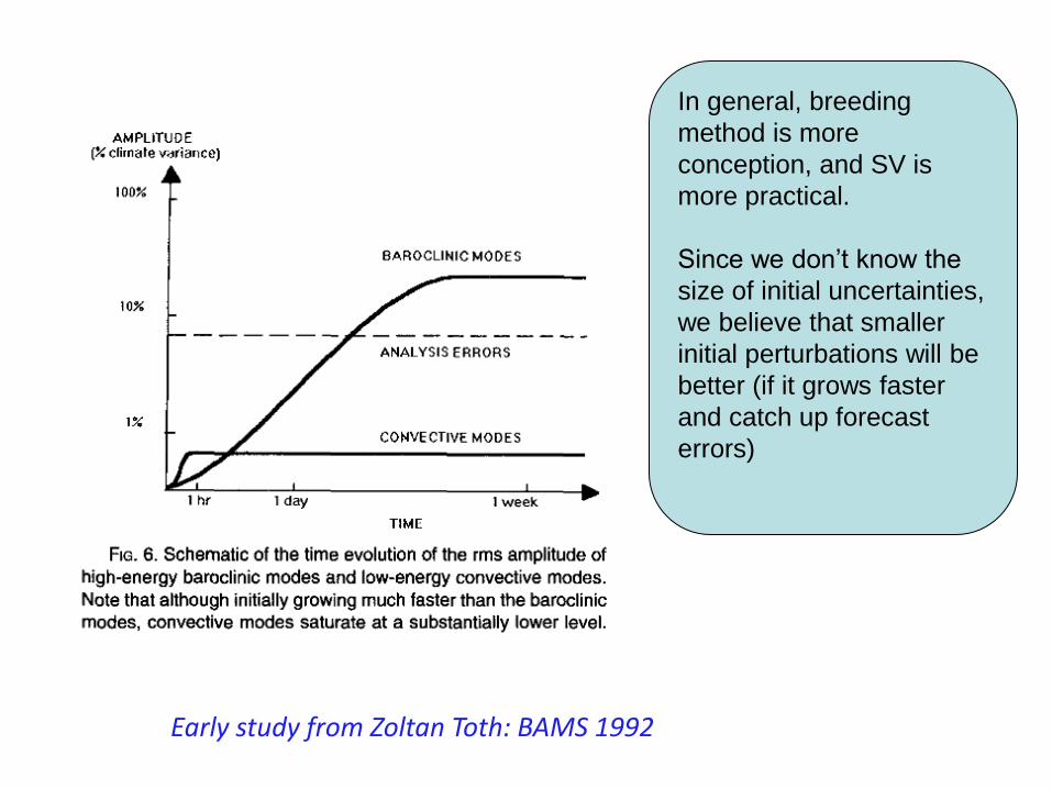
Early study from Zoltan Toth: BAMS 1992

In general, breeding

method is more

conception, and SV is

more practical.

Since we don’t know the

size of initial uncertainties,

we believe that smaller

initial perturbations will be

better (if it grows faster

and catch up forecast

errors)

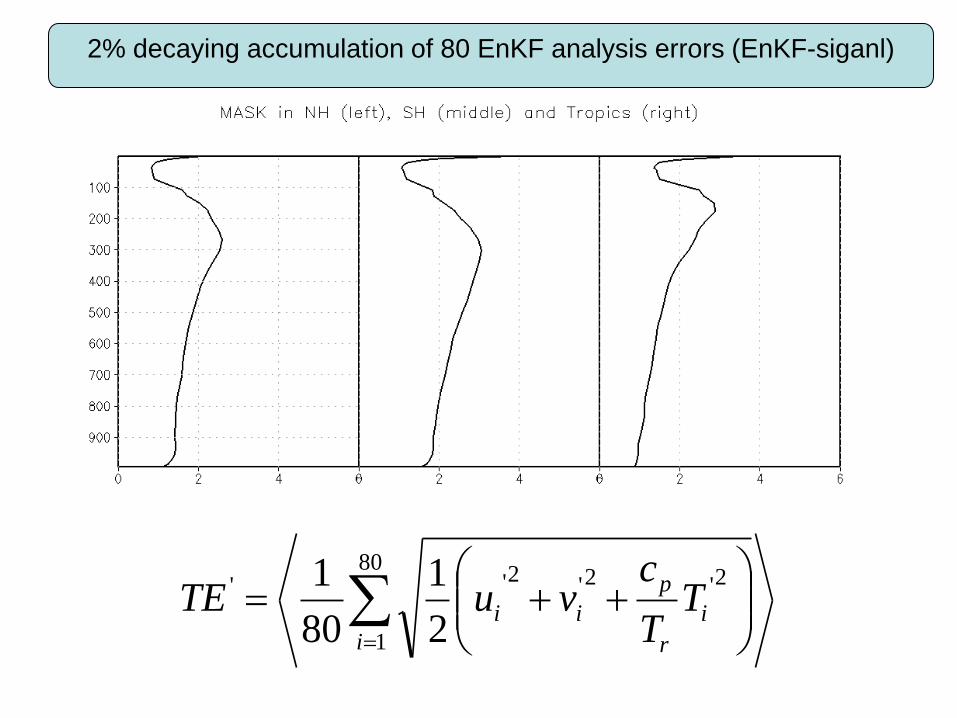
2% decaying accumulation of 80 EnKF analysis errors (EnKF-siganl)

80

1

2'2'2''

2

1

80

1

i

i

r

p

ii TT

cvuTE

Initial time: 2012090100 Black-sanl, original EnKF analysis perturbations Red-siganl, inflated EnKF analysis (approximately 36% additve) and centerization Green-f03, 3-hour forecast from inflated analysis Blue-f06, 6hour forecast Orange-f09, 9-hour forecast Purple- siganl/sanl, inflation rate for different region and different variables

Courtesy of Dr. Jessie Ma

Investigation/understanding current EnKF analysis and inflated analysis

Preliminary experiment

- Using inflated perturbations as statistical reference (3D mask) applying to ET

The skills should be very similar to EnKF’s at first try.

Note: 3D mask is decaying average (w=0.02) of total energy norm from EnKF analysis (without inflation)

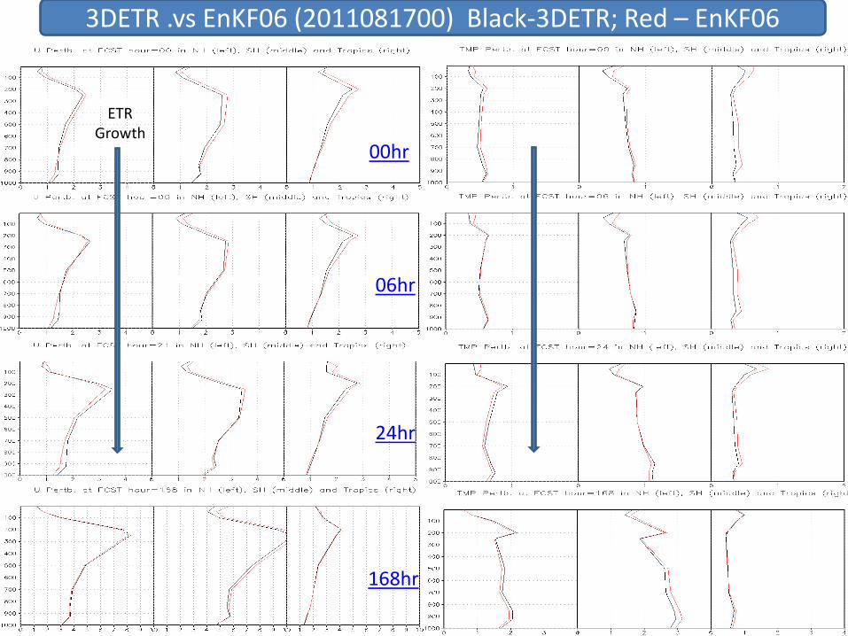
3DETR .vs EnKF06 (2011081700) Black-3DETR; Red – EnKF06

ETR Growth

00hr

06hr

24hr

168hr

Perturbations before/after 3DETR Black – before Red – after 2011081700 We should be able to tune this

Mask effect

The experiments will show the difference between ETR_2D (current operation) and ETR_3D (using EnKF analysis variance) and EnKF (f06).

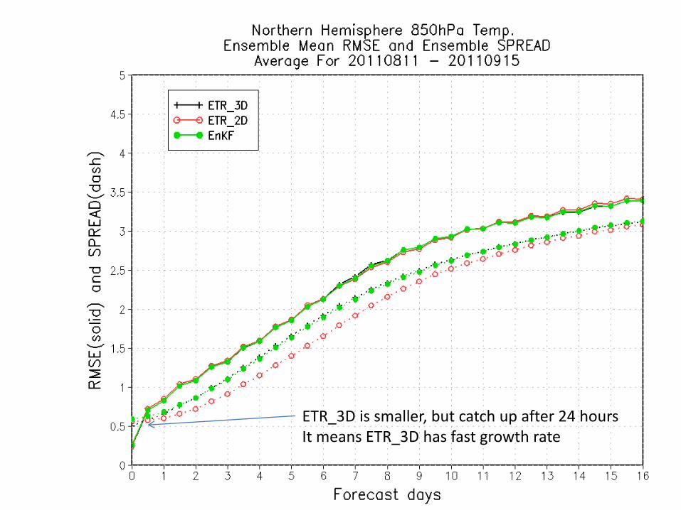
ETR_3D is smaller, but catch up after 24 hours It means ETR_3D has fast growth rate

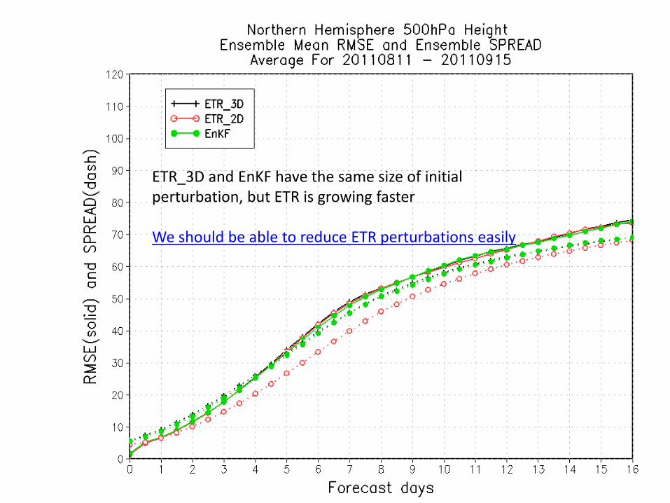
ETR_3D and EnKF have the same size of initial perturbation, but ETR is growing faster We should be able to reduce ETR perturbations easily

ETR_3D initial perturbations are much small than EnKF, but getting closer after 12 hours

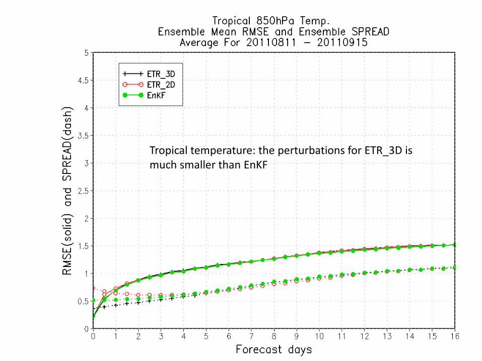
Tropical temperature: the perturbations for ETR_3D is much smaller than EnKF

For Discussion • Do we really know the analysis errors?

– Assume we know, can we use it directly as ensemble initial perturbation?

– If we don’t, what is a good initial perturbation for global ensemble forecast system?

– How to explain/understand Ricardo’s recent work? – Hybrid DA system without filtering analysis

• What is a best approach for imperfect numerical model? – Multi-model system – Multi-parameterization – Stochastic perturbation (physics) schemes

• Feedback from users – Under-forecast for extreme weather

• Future collaboration

Thanks!!!

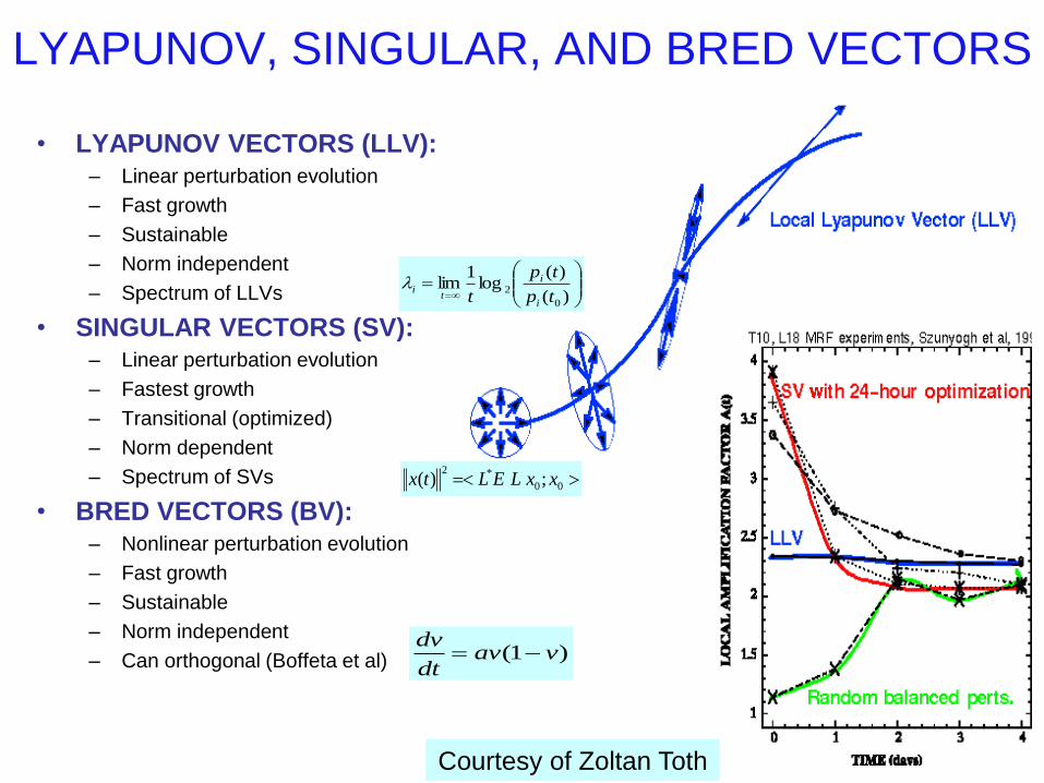
LYAPUNOV, SINGULAR, AND BRED VECTORS

• LYAPUNOV VECTORS (LLV): – Linear perturbation evolution

– Fast growth

– Sustainable


– Spectrum of LLVs

• SINGULAR VECTORS (SV): – Linear perturbation evolution

– Fastest growth

– Transitional (optimized)

– Norm dependent

– Spectrum of SVs

• BRED VECTORS (BV): – Nonlinear perturbation evolution

– Fast growth

– Sustainable


– Can orthogonal (Boffeta et al)

00

*2;)( xxLELtx

)1( vavdt

dv

Courtesy of Zoltan Toth

)(

)(log

1lim

0

2tp

tp

t i

i

ti

Lyapunov vector From Wikipedia, the free encyclopedia Jump to: navigation, search In applied mathematics and dynamical system theory, Lyapunov vectors, named after Aleksandr Lyapunov, describe characteristic expanding and contracting directions of a dynamical system. They have been used in predictability analysis and as initial perturbations for ensemble forecasting in numerical weather prediction.[1] In modern practice they are often replaced by bred vectors for this purpose.[2]

^ Kalnay, E. (2007), "Atmospheric Modeling, Data Assimilation and Predictability", Cambridge: Cambridge University Press ^ Kalnay E, Corazza M, Cai M. "Are Bred Vectors the same as Lyapunov Vectors?", EGS XXVII General Assembly, (2002) ^ Edward Ott (2002), "Chaos in Dynamical Systems", second edition, Cambridge University Press. ^ W. Ott and J. A. Yorke, "When Lyapunov exponents fail to exist", Phys. Rev. E 78, 056203 (2008) ^ F Ginelli, P Poggi, A Turchi, H Chaté, R Livi, and A Politi, "Characterizing Dynamics with Covariant Lyapunov Vectors", Phys. Rev. Lett. 99, 130601 (2007), arXiv

http://en.wikipedia.org/wiki/Lyapunov_vector


http://en.wikipedia.org/wiki/Dynamical_system

http://en.wikipedia.org/wiki/Aleksandr_Lyapunov



http://en.wikipedia.org/wiki/Ensemble_forecasting

http://en.wikipedia.org/wiki/Numerical_weather_prediction


http://en.wikipedia.org/wiki/Bred_vector




http://www.atmos.umd.edu/~ekalnay/lyapbredamsfinal.htm







http://link.aps.org/doi/10.1103/PhysRevE.78.056203





http://dx.doi.org/10.1103/PhysRevLett.99.130601





http://arxiv.org/abs/0706.0510

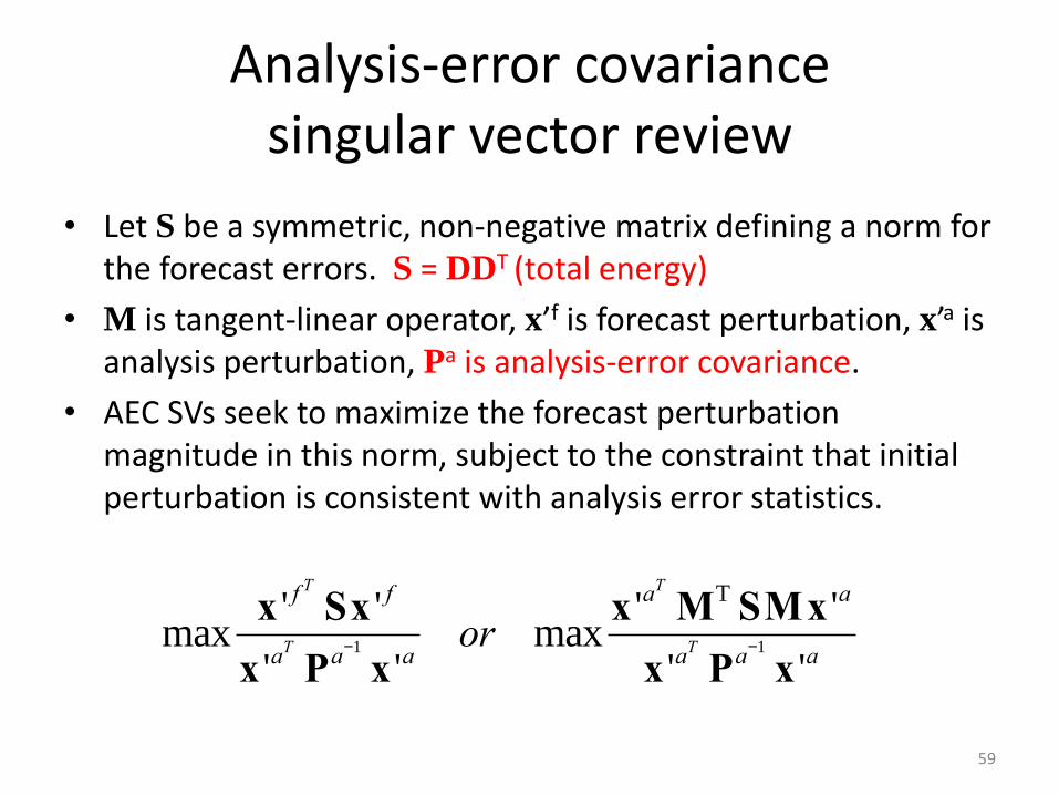
Analysis-error covariance singular vector review

• Let S be a symmetric, non-negative matrix defining a norm for the forecast errors. S = DDT (total energy)

• M is tangent-linear operator, x’f is forecast perturbation, x’a is analysis perturbation, Pa is analysis-error covariance.

• AEC SVs seek to maximize the forecast perturbation magnitude in this norm, subject to the constraint that initial perturbation is consistent with analysis error statistics.

maxx ' f

T

Sx ' f

x 'aT

Pa-1

x 'aor max

x 'aT

MTSMx 'a

x 'aT

Pa-1

x 'a

59

Ensemble Forecasting - UMCP Chaos Weather Project€¦ · Each ensemble member evolution is given...

Documents

Transcript of Ensemble Forecasting - UMCP Chaos Weather Project€¦ · Each ensemble member evolution is given...