1

Sune Mushendwa

Aalborg University – Institute of Media Technology and Engineering Science

Master Thesis: Semester 9 and 10, 2008-2009

Enhancing Headphone Music Sound Quality

i Abstract

Stereo music played through headphones comprises a narrow acoustic field which can

sound unnatural and even unpleasant at times. Various attempts to expand the acoustic

field have contained flaws which lead to deterioration in some aspects of the sound, such

as excessive coloration and other unwanted tonal changes.

In the present research a new way of achieving better sound quality for headphone music

is presented. The proposed method diverts from the familiar techniques and aims to

correct some of the current problems by using a balanced combination of assorted sound

expansion methods. These include the use of amplitude panning, time panning, and

particularly binaural synthesis.

Using the stereo format as a reference context, preference selection tests are conducted

to measure the validity of the proposed methods. Conclusions from the tests showed that

there are several factors contributing to our preference inclinations in regards to spatial

sound quality perception.

2

ii Table of Contents

i Abstract............................................................................................................................... 1

ii Table of Contents ................................................................................................................ 2

iii Table of Figures ................................................................................................................. 5

iv Appendices ........................................................................................................................ 6

1 Introduction ......................................................................................................................... 7

1.1 Externalization v/s Lateralization .................................................................................. 7

1.2 3D sound technology in music.................................................................................... 10

2 Aspects of audio signals.................................................................................................... 12

2.1 Human Sound Perception .......................................................................................... 12

2.2 Impacts of acoustic environments on sound perception.............................................. 15

2.3 Sound Localization ..................................................................................................... 18

2.3.1 Interaural differences........................................................................................... 18

2.3.2 Head Related Transfer Functions........................................................................ 19

2.3.3 Source and head movements.............................................................................. 20

2.3.4 Distance Perception ............................................................................................ 21

2.3.5 Familiarity as a factor to sound localization ......................................................... 21

2.4 Effects of background noise on sound localization and externalization....................... 22

2.5 Effects of audio file sizes on localization and externalization ...................................... 23

3 Current sound expansion techniques ................................................................................ 25

3.1 Amplitude panning...................................................................................................... 26

3.2 Phase modification – Time panning............................................................................ 28

3.3 Binaural synthesis ...................................................................................................... 29

3.3.1 Reproducing binaural sound................................................................................ 29

3.3.2 Tonal changes in HRTF cues .............................................................................. 30

3.3.3 Externalizing music using binaural synthesis....................................................... 31

4 Evaluating sound quality.................................................................................................... 37

4.1 Sound quality ............................................................................................................. 37

3

4.2 What is music?........................................................................................................... 39

4.3 Sound quality evaluation tests .................................................................................... 40

4.3.1 Results from spatial sound quality evaluations .................................................... 40

4.3.2 Relevant sound quality evaluation test methods.................................................. 42

4.4 Considerations for sound quality evaluation in this project.......................................... 43

5 Research question ............................................................................................................ 46

Can a wider acoustic field enhance the listening experience of music played through

headphones?........................................................................................................................ 46

6 Design and implementation of stimuli ................................................................................ 48

6.1 Design........................................................................................................................ 48

6.1.1 Choice of Stimulus .............................................................................................. 48

6.1.2 Song composition................................................................................................ 49

6.2 Implementation........................................................................................................... 50

6.2.1 Creating 3D sound by recording and by digital signal processing ........................ 51

6.2.2 Overview of arrangements in a soundfield........................................................... 53

6.2.3 Mixing and monitoring ......................................................................................... 53

6.2.4 Placement of vocals in the 3D soundfield ............................................................ 55

6.2.5 Placement of the instruments in the 3D soundfield.............................................. 57

6.2.6 Mastering ............................................................................................................ 58

7 Testing and evaluation ...................................................................................................... 59

7.1 Pilot test ..................................................................................................................... 59

7.1.1 Implementation.................................................................................................... 59

7.1.2 Analysis, results and conclusions from pilot test.................................................. 62

7.2 Main Test ................................................................................................................... 64

7.2.1 General outline of test ......................................................................................... 64

7.2.2 Preference selection test – short sound clips....................................................... 65

7.2.3 Preference selection test – full song.................................................................... 66

7.2.4 Additional questions ............................................................................................ 67

8 Test results........................................................................................................................ 69

8.1 Preference selection test results – short sound clips .................................................. 69

8.2 Preference selection test results – full song................................................................ 74

4

8.3 Additional questions ................................................................................................... 76

9 General discussion, conclusions and future directions ...................................................... 80

9.1 General Discussion .................................................................................................... 80

9.2 Conclusions................................................................................................................ 82

9.3 Future research.......................................................................................................... 83

10 References .................................................................................................................... 85

5

iii Table of Figures

Figure 1 - Externalization v/s Lateralization .............................................................................. 10

Figure 2 - Simplified diagram of an impulse response. ............................................................. 17

Figure 3 - Signal routing used in Wave Arts Acoustic Environment Modeling. .......................... 33

Figure 4 - Neumann KU 100 – Dummy-head Binaural Stereo Microphone. .............................. 34

Figure 5 – Sound image of the song "good friend".................................................................... 50

Figure 6 – Diesel Studios graphical user interface.................................................................... 52

Figure 7 – Bi-amp 8” stereo monitors used for mixing and mastering. ...................................... 54

Figure 8 – Positioning of backup vocals around a listener in a 3D soundscape. ....................... 56

Figure 9 - Focusrite Saffire soundcard and Sennheiser HD-210 headphones used in listening

tests ......................................................................................................................................... 59

Figure 10 - Chi square test graph for sound clips - Pilot test..................................................... 62

Figure 11 - Musicmatch Jukebox: Audio player used for playback of short sound clips ............ 65

Figure 12 - Nuendo sequencer used for playback in full song test ............................................ 67

Figure 13 - Chi square test graph for sound clips ..................................................................... 70

Figure 14 – Selection rate of 1’s and 2’s for all sound clips....................................................... 72

Figure 15 – Selection rate of 1’s and 2’s for mock sound clips.................................................. 72

Figure 16 – Selection rate of 1’s and 2’s for difficult sound clips ............................................... 72

Figure 17 – Selection rate of 1’s and 2’s for easy sound clips................................................... 72

Figure 18 – Graphs indicating an increasing preference for 3D sound clips as the test

progresses ............................................................................................................................... 73

Figure 19 - Chi square test graph for full song.......................................................................... 75

Figure 20 - Level of difficulty in distinguishing between short sound clips ................................. 77

Figure 21 – Chart indicating whether subjects perceive sound as coming from beyond

headphones ............................................................................................................................. 78

6

iv Appendices

Appendix 01 – List of spatial attributes from ADAM test…………………………………….. 91

Appendix 02 – Pilot test questionnaire………………………………………………………… 93

Appendix 03 – Results table for Pilot test……………………………………………………… 94

Appendix 04 – Final test Questionnaire……………………………….……………………….. 95

Appendix 05 – Preference Selection test Results……………………….……………………. 96

7

1 Introduction

1.1 Externalization v/s Lateralization

As technology has in recent years made it possible for portable music players to become

smaller and more efficient, it has consequently led to the ever increasing popularity of

these devices of which most play in standard stereo. Although the stereo format was

originally intended to be used with a set of two stationary speakers, it found its way to

these portable players and other headphone related music players without any

amendments to its original intended function. When music in this format is played back

through headphones they effectively narrow down the acoustic field of the sound to a

distance equal to the distance in between our ears and the sound is perceived as

coming from within the head. This is known as lateralization or in-head localization.

Lateralization takes place when there are confusing sound cues or the lack of sound

cues which the auditory system needs to determine the position or the sound source

outside the head. Due to current music production techniques music played through

headphones is in most cases bound to be lateralized. Lateralized music lacks the

important element of dimension which can result in making it sound unnatural and even

unpleasant at times - especially for sounds which lack any effects such as reverbs or

delays [3,1].

Because hearing is a dynamic process that adapts easily to assimilate with the

perceived sound [18], it seems as if we get accustomed very fast to hearing headphone

music within this limited acoustic field are able for that reason to enjoy the music to

anyway [5]. But if we were to compare the sound quality of regular headphone music

mixed in stereo to an immersive surround sound mix there would be a definite rift

between the two due to the ability of surround sound to reproduce clearer sound with

more depth and more ambience than mono and stereo. The large acoustic field in a

surround sound setting has been proven in many situations to have benefits in terms

sound reproduction quality [1].

8

A number of studies have shown that a larger acoustic field in headphones (externalized

sound) leads to better sound quality and a more pleasant listening experience [12,2,3].

Externalization in this case is the term used to describe perception of sound played

through headphones and appearing to originate from outside the boundaries of the

head. Most of these studies suggest achieving externalization by the use of real-time

signal processing algorithms that map sound from stereo signals and positions the

sound outside the head to create a spatial effect by the use of psychoacoustic principles.

These algorithms do increase sound quality in a number of cases but they also have

several drawbacks.

The results achieved when using real-time processing vary widely depending on what

type of music is being played due to the different processing involved at the recording

and mixing stage. Added effects from the externalization process often interfere with pre-

processed effects such as echoes, ambience and reverberation that had been added

during the initial mixing. Different versions of these processors can be found bundled

into audio software or can be obtained as plug-ins, but are so far seldom being used in

portable media players due to the high processing power needed to operate them.

Implementation into portable players has also been difficult partly because they need

different settings for each type of music and the players usually have a limited capacity

to facilitate custom settings.

Other studies by Fontana et al. [4,5] suggest recording of binaural sound in studio

settings by using microphones fitted into artificial heads known as dummy-heads or

KEMARs [Figure 4]. Some dummy-heads are also built with a torso. The placement of

the microphones corresponds with the position of ears in a human and can in this way

record binaural sound that can be reproduced through headphones. The problems faced

by these approaches are the huge differences between the physical characteristics of

listener’s heads, ears and torsos. These differences mean that for ideal binaural

playback there needs to be custom equalization and calibration to both headphones and

recording microphones to fit each individual. In reality it can work in laboratory

environments but this time-consuming approach is not an option for mass production of

music. On the other hand reproducing binaural recordings on loudspeakers is more

robust. Here the listener needs to be situated in particular position known as the sweet

spot usually forming an equilateral triangle with the loudspeakers. But even when not

9

situated in the sweet spot the sound can still appear to have subtle improvements

compared to regular stereo.

This project takes a new approach to the expansion of the acoustic field of music played

through headphones by putting the music producer at center stage. Music being an art

form will need input not only from a technical perspective but an equally important role

should come from an artistic and a user’s point of view. In the process of creating a

wider acoustic field the music producer will still be in charge of the final outcome of the

music. This approach is even more important taking into account multidimensional

attributes in music such as the overall spatial audio fidelity.

Studies by Zielinski et al. [6] have shown many hedonic judgments are prone non-

acoustical biases like situational context, expectations and mood. This suggests the

actual arrangement of sound in a 3D space might not be as noticeable to an uninformed

listener who might pay very little attention to the details of the song; instead the listener

may perceive it as a complete entity while still having certain expectations to how the

song should sound.

In this project sound expansion and externalization is achieved by a balance of stereo

mixing and the use of binaural sound from the very beginning of the recording and

mixing process. The approach will allow for strategic placement of sounds both inside

and outside the normal acoustic field of headphones while retaining greater control of

the mixing process and the final result as will be perceived by the end user. This should

also allow for better control of the perceived sound source distances and direction by

taking into account the effects of background noise and sound masking. These tend to

have a big impact on the perception of sound also in regards to music. In this case

musical instruments and vocals mask each other and can likewise be regarded as

background noise.

A good balance of stereo and 3D sound should as well allow the songs to be played with

improved sound quality on both loudspeakers and headphones without any adjustments

or equalization to the track. When comparing tracks mixed with this approach to regular

stereo the anticipated outcome is to attain better envelopment, clarity and a more

enjoyable listening experience of music.

10

Figure 1 - Externalization v/s Lateralization

1.2 3D sound technology in music

Since the origin of binaural technology there have been advances in the various fields

that make use of this technology. This is especially true in the past few decades which

have seen an increasing simplicity to access powerful computers and digital signal

processing software [7], cheaper and better microphones for binaural recordings, and

undoubtedly the growth of the internet which has given many people the opportunity to

experience the technology as well as learn about it. However, the music industry has not

made much advancement in integrating 3D sound technology with the production of

music but has instead maintained the standard stereo format. It is rather difficult to find

references to companies and individuals whose work on integrating psychoacoustics

principles and music creation has been widely acknowledged.

Roland Corporation (a manufacturer of electronic musical instruments and software) had

an attempt at building a hardware mixer which would allow for placement of sounds

outside the range of stereo speakers by using psychoacoustics. It never became a very

popular instrument partly due to a very high price and the limited interest in the spatial

effects it produced. Its production was eventually cancelled.

11

Some software based companies advertise their products as having the ability to “greatly

enhance stereo as well as multi-channel music” but these solutions only act as “makeup”

to an existing product [14,20,8] and do not make an attempt at redesigning the core file

formats used in the music industry today.

Despite the advances that have been made with 3D-sound technology and the music

industry there is a lack of examples of music produced for a better headphone listening

experience. Perhaps there are some underlying reasons which contradict or clash with

the theory that a wider acoustic field can enhance the listening experience of music

through headphones. So far it seems that the technology remains mainly a hobby to

many audio enthusiasts rather than serious attempts to combine the two.

12

2 Aspects of audio signals

2.1 Human Sound Perception

Human sound perception is a complicated mechanism that is affected by both internal

and external factors. It is possible to listen to any sound either in terms of its attributes or

in terms of the event that caused it [9]. The auditory system can link a perceived acoustic

event through previous experience to an action and a location or it can perceive the

attributes of the sound itself. The actual distinction is between the two ways of listening

is based on experiences, not sounds [10].

Perceiving Sound As An Event: Human beings have developed their auditory skills

from everyday listening. Through experience we learn to notice the audio cues that

concern us as events that we can react to such as the sound of an approaching car or

the sound of the pot boiling over in the kitchen or the sound of thunder. The exact

mechanisms that lets us differentiate and characterize the fundamental attributes of such

acoustic cues is still not well known to us despite thorough studies in relevant areas

concerning the subject – most notably is the research in sound source localization and

timbre perception [9]. This type of everyday listening is what seems to give us the ability

to perceive sound source direction and distance – localization. Through localization we

are able to experience externalization/ out-of-head localization.

Localization takes place because all of the sounds that we perceive in everyday life have

been to at least some extent attenuated. The attenuation is caused by the medium it

travels through and the surrounding environment before reaching the eardrums from the

original sound source location. This is because the listener must inevitably occupy a

different location than the sound source [2], and so the spatial component of sound

caused by a physical change in distance and location produces a number of changes to

the acoustic waveforms that reach the listener. Even when listening to your own voice

alterations will occur to the sound as a result of the vocal chords being located in a

different place than the ear drums. This is why our own voices tend to sound unfamiliar

when we hear them recorded for the first time.

13

We seem to perceive most of the differences that occur in the sound at a subconscious

level and interpret them as indications of the sound source location rather than merely

duration, spectral or tonal changes in the sound [12,10,2]. The perceptual dimensions and

attributes of concern correspond to those of the sound-producing event and its

environment, not to those of the sound itself [9].

Perceiving Sound by Its Attributes: On the other hand humans also perceive sound

by listening to its pitch, loudness, timbre etc. This is the type of listening in which the

perceptual dimensions and attributes of concern have to do with the sound itself and is

traditionally related to the creation of music and musical listening [9]. With musical

listening, unintended alterations that occur with either of the sound components will

seemingly be more consciously audible. More audible than if the sound was perceived in

terms of the event that caused the sound.

Unlike everyday listening, listening to most music requires that the music itself has

unified sound consistency and an established order in its overall composition for it to

sound adequate. Even the tonal modifications that come as a result of the spatial

components of sound can also make any irregularity more noticeable and even

undesirable – whether it’s in the recording or reproduction stage. For example the large

distance between a singer and microphone when recording music can easily be noticed

due to an increase in levels of relative-to-direct reverberation [21], an effect that

otherwise wouldn’t have gained much attention in everyday listening. Humans can in

some cases consciously choose whether to listen to a sound either in terms of its

attributes or in terms of the event that caused it. Music can be listened to as everyday

sounds and everyday sounds can be perceived by listening to the attributes of the

sound.

Non Linearity in Human Sound Perception: Knowing that a human is the ultimate

recipient of a sound signal in this project, it is worth pointing out the non-linearity of

human sound perception. There can be a difference between the acoustically

measurable characteristics at the sound source and the percept at the listener’s end. It

applies for frequency, amplitude as well as the time domains [3]. It is not possible to

always rely on a mechanical or mathematical approach in order to examine human

sound perception and perceived sound quality. For instance the perceived loudness

does not necessarily correspond directly to the actual intensity changes at the sound

14

source. Neither does numeric assessment of the frequency content always give clues to

the subjective pitch perceived [3].

There are a number of models which have been developed for objective testing of sound

quality from virtual sound sources. An example is the binaural auditory model for

evaluating spatial sound developed by Pulkki & Karjalainen [11]. The model is based on

studies from directional hearing which are then tuned with results from psychoacoustic

and neurophysiologic tests. In the model, the perceived sound resulting from the function

of different parts of the ear (such as the ear canals, middle ear, cochlea and hair cells),

are modeled by different filters that replicate the perceived attenuations in the sound as

a function of distance and direction.

Although the model has proved to be effective in achieving its objectives it has a major

drawback in the sense that the model only has the ability to predict the positions of

virtual sound sources. It does not predict sound quality in terms of the sound

characteristics that let the ear distinguish sounds which have the same pitch and

loudness or the level of comfort the listener experiences. Nor does it predict sound

quality in the sense of listeners’ emotions to enjoyment or pleasantness.

In short human perceptual tendencies include: Perceiving sound in terms of its

attributes, perceiving sound in terms of event that caused it, and the non-linear

characteristics of sound perception. Because of these varying perceptual tendencies the

main premise for determining quality of sound can not exclude subjective quality tests

that take into account the human auditory system. Subjective tests should in effect be at

the center of all analysis; even the simplest assessment on whether sound quality has

improved or degraded requires human subjects [3].

This thesis intends to use the changes in sound caused by 3D positional rendering for

externalization/ expansion of the acoustic field in headphones. The modifications made

to the sound should be for improving quality and not simply expanding the acoustic field.

But when used excessively or applied incorrectly, spatial modifications can have the

opposite effect and lead to deterioration of the sound quality despite a larger acoustic

field being obtained [4]. Therefore it is important to first understand how the location and

distance cues that lead to externalization function, and how they affect the overall sound

quality in regards to a musical composition.

15

2.2 Impacts of acoustic environments on sound perception

An acoustic environment provides many valuable cues that help in creating a holistic

simulation of an acoustic scene by adding distance, motion and ambience cues as well

as 3D spatial location information to the sound [12,2]. The cues are due to several factors

which cause changes in the acoustic waveforms reaching the listener, these include the

room size and material, sound source intensity, sound frequency [12], and also

experience [13].

There are of course different types of acoustic environments such as outdoor

environments which color the sound differently as a result of minute levels of

reverberation compared to indoors environments. Specially modified rooms called

anechoic chambers can be used to simulate a free field, ideally with no reflections at all.

These are rooms which are treated with sound absorbing and sound diffracting materials

that eliminate sound reflections. There are also half anechoic rooms with solid floors

which would give the same effect as recording out on a big open field.

But for reasons of clarity, “acoustic environments” in this case will refer to indoor

environments with surfaces from which the sound waves can be reflected and absorbed

– or in other words, spaces with reverberation. This is a characteristic which defines

most acoustic environments [14]. Reverberation can both assist as well as impede a

persons sound localization capabilities within that particular space.

Reverberation in a room occurs when sound energy from a source reaches the walls or

other obstacles and is reflected and absorbed multiple times in an omnidirectional or

diffused manner. Reverberation and especially the ratio between direct-to-reverberant

sound is possibly the most important cue for externalizing a sound [10]. It is more likely

that late reverberation will be masked than individual earlier reflections and therefore

without significant effect in externalization [14]. Late reverberation is generally considered

to be reverberation which has dropped 60dB below the original sound. It usually occurs

about 80ms after the direct sound but this depends on the proximity of reflecting

surfaces to the measurement point [Figure 2][14].

Localization in reverberant spaces depends heavily on what is known as the precedence

effect, a perceptual process that enhances sound localization in rooms. The precedence

16

effect assumes the first wave front to be the direction from which the sound originated as

it should be shortest and therefore the direct path from the origin. The effect is thought to

work as a neural gate which is triggered by the arrival of sound, for about 1ms it gathers

localization information before it shuts off to subsequent localization cues [15].

Localization of transient sounds is more accurate compared to localization of sustained

sounds in which reflections can be confused with the direct sounds [16].

The direct-to-reverberant ratio is mainly related to subjective distance perception

whereby the direct sound decreases by about 6dB for every doubling of distance, the

reverberant sound only decreases with about 3dB for the same increase in distance [17].

When there is an increased distance between the sound source and the listener, the

direct sound level decreases significantly but the reverberation levels decrease at a

smaller rate.

What affects reverberation is in many ways directly connected to the characteristics that

typify a particular acoustic environment. Room size and the original sound source

intensity are directly proportional to the duration of the reverberation. Sound Frequency

also has an effect whereby lower frequencies tend to have a longer reverberation time

than higher frequencies but this is in turn affected by the level of absorptiveness of the

reflecting materials within the acoustic environment. All of these together with other

aspects such as the room shape add substantially to the modifications of the spatial

temporal patterns and timbre of the sound within the space. As a result of these

modifications it allows for our cognitive categorization and comparison of acoustic

environments [14].

Experience can be gained from exposure where the listener adapts to the reverberation

characteristics of the given room without explicit training or feedback. Hearing is very

adaptive to different acoustic environments but can also be misleading. A study in

reverberation by Shinn-Cunningham [18] shows that listeners calibrate their spatial

perceptions by learning a particular room reverberation pattern in order to suppress or

fuse particular phases of the reverberant sound so as to construct a single event. The

single sound event can then be localized to a higher degree of accuracy compared to

sound containing disruptive spatial cues from echoes.

Research by Griesinger [19] concerning virtual audio localization through headphones

has shown that motivated listeners using non-individualized playback can convince

17

themselves that the binaural recordings work, even though the headphone system

usually needs to be matched to the individual users in order to reproduce accurate

sound source positions. The research showed that at times localization of virtual sources

may even come down to the willingness and ability to suspend conflicting sound source

cues or the lack of it.

Reverberation plays an unavoidable part in sound localization and in creating a more

realistic acoustic environment but also plays a very delicate and often incompatible part

in music production. Typically in music production dimension effects (which include

reverberation) will be applied to dry sound as “makeup” with varied results depending on

what type of reverberation is applied [20].

Dimension can also be captured during the recording stage by using room ambience,

but it is usually created or enhanced during the mixing process because once

reverberation is added to the actual sound file it is almost impossible to get rid of.

Dimension effects are applied very often but only under very stringent and controlled

conditions taking into account equalization, pre and post reverb times, delays,

modulated delays as well as the reverberant-to-direct sound ratio [20,21]. The

reverberation settings in a music track may have nothing to do with the way actual

reverberation is perceived in a real space but they are used as long as the music track

sounds good. The idea “Do anything as long as it sounds good” is the unwritten rule of

most music producers and a good result will usually come down to having a good ear

rather than technical abilities.

Figure 2 - Simplified diagram of an impulse response.

D = direct sound. ER = early reflections > 0 and < 80ms. LR = late reflections > 80ms. The late reverberation time is usually measured to the point when it drops 60 dB below the direct sound. [14]

18

2.3 Sound Localization

Sound localization is the ability of our auditory system to estimate the spatial position of

a sound source. Localization primarily relies on the fact that humans have two ears but

localization is also possible with only one ear but at the cost of reduced accuracy [48,3].

Below are a number of cues that facilitate localization. Implementing these cues to the

tracks of recorded music is a major objective in this thesis as a means to achieve

externalization and overcome lateralization.

2.3.1 Interaural differences

Interaural Time Difference (ITD) and Interaural Intensity Difference (IID) are respectively

the most important factors in localization of sound on a lateral plane. With sound source

being at 90 degrees azimuth it will take a maximum of approximately 0.63ms longer to

reach the ear further away from the sound source. Azimuth is the angular distance along

the horizon between a point of reference, usually the observer's bearing, and another

object [61]. This tiny difference in time is detected by the brain and interpreted as a

direction rather than a time difference. Likewise, the intensity of the sound reaching the

ear (IID) further away from the source will be diminished and this difference is

interpreted as both direction and distance to the sound source[14].

However interaural time difference and interaural intensity difference does not apply to

all sound frequencies. ITD can usually be detected below approximately 1000 Hz and

only when a sound wave is smaller than the diameter of the listeners head will the sound

intensity be diminished as a result of the head acting like an obstacle. Sound waves with

a longer wavelength at a frequency of approximately 1500 Hz and below will diffract

around the obstacle. The sound wave diffraction causes the difference in intensity to be

minimized hence reducing the effect of localizing the sound source [14].

A practical application that is an outcome of our inability to localize low frequencies

sounds or bass is the surround sound system. Here the bass or low frequencies are

channeled into one speaker known as the sub-woofer which can be placed

independently of the position of the rest of the speakers without affecting the complete

19

intended sound image [1,22]. This setup allows the center, left, right and surround-

speakers to reproduce only the higher frequencies and therefore they can be smaller in

size. The bass speaker or subwoofer usually needs to be bigger in size to reproduce the

lower frequencies; hence only one large speaker is required instead of five large

speakers.

The same principle is also applicable to placement of sounds in a 3 dimensional space

to be reproduced through headphone. Our inability to detect sound source directions of

low frequency sounds means that when creating a 3D soundscape the actual positions

of low frequency sound sources become irrelevant.

2.3.2 Head Related Transfer Functions

Head Related Transfer Function - HRTF is a filtering process that sound undergoes

before reaching the eardrum and the inner ear. HRTFs do not necessarily need two ears

to function [3]; instead its mechanics lay in the attenuations of the sound caused by the

shape of the ears, head and to some extent the torso [14].

The asymmetry of the pinnae (the folds of the outer ear) cause spectral modifications,

micro time delays, resonances and diffractions as a function of the sound source

location that translate into a unique HRTF[14]. In this filtering process the folds of the

outer ear cause tiny delays of up to 300 microseconds and also change the spectral

content to differ considerably from that of the sound source. The attenuations to the

sound that eventually reaches each eardrum function to enhance the sense of sound

source direction [14,23]. The altered spectrum and timing of the sound is recognized by

the listener as spatial cues.

The head related transfer function is particularly important for vertical localization where

ITD and IID can end up with localization errors or situations known as reversals or cones

of confusion. Reversals can happen when the distance from the sound source to each

ear is the same and there is no significant time difference or intensity difference that can

be detected [12,14]. For example a sound source located 2 meters in front of the listener

will transfer equal amounts of energy to each ear and will also take equal time to reach

ear as if the sound source was located 2 meters behind, above or even below the

20

listener. But by filtering the sound and altering the frequency spectrum depending on the

direction from which the sound originates, the auditory system can better determine the

actual direction of the sound.

2.3.3 Source and head movements

Head Movements are another way for us to improve sound localization. When there is

ambiguity as to where the actual sound source is located we tend to turn our heads in an

attempt to center the sound image; this in turn minimizes the interaural time and intensity

differences that we perceive [14,24]. Head movements can by themselves not determine

the location of a sound source but are rather used in combination with ITD, IID and

HRTFs to enhance localization.

The effect of head movements is only true for physical or real sound sources and may

not apply to most virtual sources such as those reproduced by headphones. The reason

is that the with the movement of the head the virtual sound image will move as well as it

is dependant on its orientation but the spectral image will remain constant. More

advanced methods of reproducing binaural sound through headphones take into account

head movements in real-time but these setups remain to be mainly used in laboratory

environments.

To a certain extent Sound Source Movements give a similar result in solving

localization ambiguities to the perceived sound source as head movements. The

difference is that in this case the head is static and the sound source is dynamic. A

moving sound source on the other hand also causes what is known as the Doppler Shift

or the Doppler Effect. In relation to sound this is the change in pitch of the sound

depending on the direction and speed of the sound source, the listener, the medium or a

combination of all of the above. [14,25]. The Doppler shift is easily noticed for instance on

a fast moving vehicle with sirens turned on, as it approached the pitch of the sirens goes

up and at the instance when the vehicle has passed the pitch decreases again.

21

2.3.4 Distance Perception

Sound source distance is vital in maintaining a sense of realism in both real and virtual

sound environments. It usually involves the integration of multiple cues including spectral

content, reverberation, loudness, and cognitive familiarity [14]. Loudness or intensity is

the primary cue to a sound source distance but more so for unfamiliar sounds than

sounds that we are frequently exposed to. Intensity of sound or sound pressure level

from an omnidirectional sound source follows the inverse square law which means that

the sound intensity would drop 6dB for each doubling of the distance from its source

[14,26].

Spectral changes also provide information to sound source distance; in this case the

higher frequencies are diminished more than low frequencies over a distance due to

factors such as air and humidity. The differences are usually not audible to the human

ear over shorter distances of few centimeters but rather over longer distances [14]. For

sound sources extremely close to the ear the low frequency interaural differences

become unusually high, for example an insect buzzing in your ear; this is used as a

major cue for sound sources at very close range [27].

The perception of distance is also affected by the relative levels of reverberation as

discussed in section [2.2 Impacts of acoustic environments on sound perception].

2.3.5 Familiarity as a factor to sound localization

Familiarity as well is a very powerful cue to both absolute and relative sound

localization. In the case of sounds that we can relate to, familiarity becomes one of the

most important factors for determining distance [12,14]. We also tend to associate the

sound source to visual cues which we know from past experiences can produce the

particular sound. For this reason we are able to experience effects such as the

ventriloquism effect which can cause the perceived direction of an auditory target to be

directed to a believable visual target over angular separations of 30 degrees or more [28].

But even in the case where there are no visual references, experience can play a major

role in determining sound source distance and direction independent of sound pressure

22

level as long as the sound can be associated with a particular distance or location from

previous experiences. For example a whisper will be associated with a shorter distance

to the sound source than shouting although the opposite should be true if only sound

intensity was to be taken into consideration [14]. This implies that any realistic

implementation of distance cues into a 3D sound system will most likely necessitate an

assessment of the cognitive associations for the particular sound source.

2.4 Effects of background noise on sound localization and externalization

When modeling an acoustic environment it is important to consider that the efficiency of

the human auditory system to accurately localize sound can be influenced by a number

of factors. One of the factors is the presence of other sounds.

Localization can be affected either by an overload of cues or by not being able to

accurately perceive the cues from a particular signal such as when a weak sound is

masked by a louder one. This subject is especially important to take note of in this thesis

as it deals with music which in general tends to contain many different sounds

reproduced at the same time. This could mean that when creating the externalized

musical experience the sounds within the song itself may actually impede localization of

other sounds and hence affect externalization as a whole.

Perceptual overload: It is estimated that a maximum of only about 6-8 separate sound

sources can be localized at one time by the human auditory system [70]. With an

increased number of simultaneous sounds reaching the ear from different directions it

becomes harder to determine the individual sound source positions. This is true for both

perceptual sounds as well as physical sounds. A perceptual sound is a sound that a

human perceives as one sound although there may be more than one actual sound

source [29]. For instance the key of a piano contains many wires each producing a sound

but it is perceived as one sound by the ear.

Audio masking: Another case is with audio masking. This happens when the

perception of one sound is affected by another sound reaching the ear at the same time

making it less audible. Simultaneous masking is reached at the point when the weaker

sound becomes inaudible. In an experiment conducted by Lorenzi and Gatehouse [30] to

23

determine the ability to localize sound in the presence of background noise, it was

observed that localization accuracy decreased with an increase in background noise.

The experiment was conducted using clicks which were presented together with white

noise. Results showed that localization remained unaffected with low signal-to-noise

ratios but deteriorated with a gain in the noise levels especially when the noise was

presented perpendicularly to the ear. It was suggested that this could be because of a

reduction in the ability to perceive the signal at the ipsilateral ear and thus interfering

with the IID level. On the other hand, low-frequency signals are less resistant to

interference from noise than high-frequency signals when noise is presented at the same

position.

2.5 Effects of audio file sizes on localization and externalization

Most recordings will contain unwanted noise to at least some degree. This can be

caused at any stage by the recording space, microphones, cables, etc. The impact of

noise in standard studio procedures is minuscule but can escalate in the process of file

compression to reduce file sizes.

Compression is necessary in this project if any tests are to be conducted using a

portable music player. Most portable players may not have large storage capacities

which can handle standard uncompressed files. Likewise, if any files are to be

transferred over the internet, compression may be necessary as well.

Most of the music shared or sold online undergoes some kind of compression aimed at

reducing the size of audio data. This lets it occupy less space on disks and less

bandwidth for streaming over the internet [31]. The amount of compression used to

reduce file size is limited as the file size is directly related to the audio quality; a balance

has to be established between the eventual file size and the sound quality needed.

It is worth noting that a stereo file and a 3D sound file will both use roughly the same

amount of space when saved as a PCM wave file or as a compressed version as they

both use only two channels each. PCM (Pulse Code Modulation) files are what are

considered to be standard high quality or CD quality audio files [31]. These files are

24

usually very big and therefore require large amounts of storage space which might

sometimes not be available.

A normal 4 minute stereo music file in PCM format would be about 42 MB but when

encoded to mp3, AAC or alike with a bit rate of 192 kilobits per second it will be only

around 6 MB. Most types of compression will affect the playback quality of the sound file

in a negative way. This can be a particular setback in lossy encoding (perceptual audio

coding) where compression is done by actually removing information in the audio file [31].

Lossy encoding is possible due to the psychoacoustic phenomenon known as frequency

domain masking. Softer sounds within the same frequency range will be masked by

louder sounds rendering them inaudible. If too much compression is applied to the

sound files there will eventually be sound deterioration and an addition of noise known

as quantization noise. In the case of binaural or 3D sound files the removal of audio

information and the resulting addition of noise can eventually lead to a loss of

localization capability during playback [30].

However, another form of compression known as lossless encoding does not

compromise the quality of the original recordings [31]. It functions by compressing the

entire stream of audio bits without removing any of them. The audio after lossless

compression is in every way identical to the audio before going into the encoder. The

amount of compression possible with this type of encoder is on the other hand much

less than with lossy encoders.

Although lossy compression causes degradation to the sound it is usually not noticeable

to most listeners if the bit rate remains above 192 kilobits; and especially hard to notice

without high-end reproduction systems. Eventually which type of compression is to be

used depends on how much storage space and bandwidth there is, and how much

sacrifice can be made to the sound quality.

25

3 Current sound expansion techniques

Replication of multiple sources at different positions in space plays a major part in

recording and production of music and soundtracks. It is usually applied to recorded

music and other audio to recreate or to synthesize spatial attributes to the listener by

spreading the sound image over a larger acoustic field. The main aim with sound

expansion or spatial audio rendering is to make it sound better. In music terminology it is

referred to as panorama – placing the sound in the soundfield - to create clarity and to

make the track sound bigger, wider and deeper [20].

A spatially encoded sound signal can be produced by either recording an existing sound

scene or synthesizing a virtual sound scene. Each of the alternatives contains many

variations of reproduction with different results. Depending on the technique used, the

virtual audio sources can be achieved as point-like sources to a defined direction and

distance or simply give a spacious feeling to the audio without precise localization cues.

The latter despite having bad localization and readability of the scene usually gives a

good sense of immersion and envelopment. The former mentioned expansion technique

provides precise localization and good readability but lacks immersive qualities [32].

Much research has been carried out in sound expansion for headphones as well as

stereo and multiple speaker setups. The main focus in most research has been with the

use of amplitude panning, phase modification, HRTF processing [33] and also by

considering the acoustic environment as discussed in section 2.2.

The efficiency of the sound expansion techniques is normally determined by evaluating

the directional quality of virtual sources [41]. This describes how precise the perceived

direction of a virtual source is compared to the intended direction. There will generally be

differences in the cues from the real sources and the virtual sources which can lead to

the virtual source sounding diffuse. In terms of quality this is to say that the narrower the

width of the virtual sound source in the intended direction, the higher the quality

achieved. Ideal quality is reached when the auditory cues of the virtual source and the

cues from a real source are identical.

26

However, this type of quality assessment only takes into account the attributes derived

from objective analysis of the sound. It can be practical in evaluating certain aspects of a

piece of music such as clarity of different instruments but does not give a comprehensive

evaluation on how good the whole song sounds to the listener. The use of exclusively

perceptual measures to evaluate audio signal quality can not be enough to explain the

perception of sound quality to an individual. It must instead include research that takes

into account the individual and cultural dimensions of human value judgment [34].

The following sections [3.1 - 3.3.3] look at some of the main techniques used for sound

expansion in a variety of audio playback systems including headphones. Some of the

discussed techniques are then used in this project to achieve externalization.

3.1 Amplitude panning

Amplitude panning is the most widely used technique for placing a monaural signal in a

stereo or multichannel sound field. It needs at least 2 separate audio channels to

function such as headphones or stereo loudspeakers but also functions with a higher

number of audio channels such as in surround sound systems.

Amplitude panning can be used for different loudspeaker setups whether it is a linear,

planar or 3 dimensional soundfield. Irrespective of which setup is considered, the sound

image is perceived as a virtual source in the direction which is dependent on the gain

factor of the corresponding channel [33]. From this basis there has arisen more complex

amplitude panning configurations aiming to recreate more authentic auditory scenes by

taking advantage of a larger number of loudspeakers. These include Ambisonics, Wave

Field Synthesis, and Vector Based Amplitude Panning (VBAP).

Wave field synthesis [35,36] converts the whole sound field into a listening room by using

a very large number of loudspeakers, usually up to 100. This is in itself a very effective

technique that creates virtual images independent of the listener’s position. But the

system is not practical in most circumstances due to its shear size and difficulty in

implementation, and so it has largely remained to be used in sound laboratories.

27

Likewise, Ambisonics [37,38] and Vector Based Amplitude Panning [39] are not typical

systems partly because of their hardware requirements and also because of difficulties

in implementation. Although the actual methods used in these more complex sound

expansion techniques can only operate with loudspeakers, the same methods applied to

amplitude panning for stereo channels often works well for both loudspeakers and

headphones.

In stereophonic amplitude panning the location of the sound image produced by the

loudspeakers, also known as panning angle will appear on a straight path between the

two loudspeakers. The sound image has a narrow sound image width with high quality

localization information [33]. Amplitude panning in itself will very rarely expand the sound

beyond the perimeter of the loudspeakers [40] and in case of headphones it seldom leads

to out-of-head localization/ externalization. But it is still very effective in separating and

spreading concurrent mono signals within this space to create a more pleasant listening

environment.

According to the duplex theory the two frequency-dependent main cues of sound source

localization are the ITD and the IID [41]. Low frequency ITD and also to some extent

high-frequency IID cues are often the most reliable cues for localizing virtual sound

sources in stereophonic listening. Above approximately 1500Hz the ITD cues can

become degraded, and between the frequencies of about 700Hz – 2000Hz the IID cues

can become unstable resulting to perceived directions outside the span of the

loudspeakers [42]. Other studies [33] have shown that the temporal structure of the signals

changes the prominence of cues especially where there is discrepancy. Localization of

sustained sounds tends to be more accurate with IID while transient sounds are better

localized with ITD.

There are a number of equations that are used to estimate the sound source location by

the gain factors of the loudspeakers [43,44,45] but the exact sound source position will also

depend on factors such as the acoustic environment, the listeners position and direction,

etc which is difficult to include into a single equation. Some of the equations only

function correctly in establishing the sound source within specific frequency ranges

[33,40]. Due to the design of headphones many of these variables affecting loudspeakers

do not need to be taken into account; therefore the result can be better predicted with

the use of mathematical formulas. In any case these formulas can not be applied as an

28

overriding rule for positioning sound in a music track. Music often also relies much on

subjective inputs and other factors such the correct phase of the signal in order to get a

good sound [1]. For example music producers will often pan stereo mixes while

monitoring in mono despite reduced sound quality, but can in turn easily detect phase

disparities.

Besides the equations that determine the position of the sound source there are the

equations which determine the amplitude of the perceived sound image in relation to its

position. The stereo pan laws [46] estimate a perceived increase of about 3dB when the

sound image is panned to the center. This is as a result of doubling up the two similar

signals rather than if the signal was panned hard left or hard right and playing through

only one loudspeaker. The perceived increase is also affected by the acoustic

environment whereby in acoustically controlled rooms the summing of signals in the air

occurs more accurately and an increase of 6dB is a more precise estimate. Because of

these variables a typical control for constant power in amplitude panning will be between

3 – 6dB. Most music hardware and software mixers leave the settings of this variable to

be set by the producers as it is usually down to the individual ear and the surroundings

to what amount of attenuation will yield the most pleasing results in stereo panning.

3.2 Phase modification – Time panning

Modifying phase information is sometimes used as a panning technique and as a spatial

effect for widening the stereo image by placing phantom images outside of the normal

range of the loudspeakers. Externalization can be achieved in headphones using this

technique. When a constant delay is applied to one channel in a stereophonic setup, the

sound source is perceived to originate in the direction of the loudspeaker that generates

the earlier sound signal. The biggest effect is attained with a delay of about 1ms [33].

However it has been shown that the perceived directional cues of the virtual sources are

frequency dependent and therefore the effect is not consistent with all frequencies.

Time panning/ phase modification is often used in real-time algorithms to process stereo

signals to get a wider acoustic field. The process in such instances does not discriminate

between individual sounds but rather affects the sound image as a whole. This can often

29

lead to degradation of the spatial and timbral aspects of the original stereo mix [1,14]. The

quality of source direction is generally very poor as a very wide virtual image is formed.

On the other hand sound envelopment is quite good using this panning technique.

3.3 Binaural synthesis

3.3.1 Reproducing binaural sound

The cues that the ears pick up as a result of direction and distance from the sound

source can be replicated and added to a sound signal. This process is known as

binaural synthesis. Binaural synthesis allows for monophonic signals to be positioned

virtually by the use of only two channels in any position; at least theoretically. The

modified signal can then be reproduced with the effect of the desired direction by using

either headphones or stereo speakers. Binaural synthesis works very well when the

listener’s own HRTFs are used to synthesize localization cues but this is a time-

consuming and complicated procedure. Instead, generalized HRTFs are used in most

cases [12].

For the use of stereo speakers interaural cross-correlation causes confusion as the

sound from a speaker reaches the contra lateral ear. A method to control the signals

reaching each ear is by using cross-talk cancellation. It works by adding an inverse

version of the cross-talk signal to one of the stereo signals with a delay time which

equals the time needed for the sound to travel to the other ear [14]. Its effects are rather

hard to control unless playback is in rooms with very little reverberation – where the

reflected sound energy will not interfere with the intended spatial effects. The positions

of the speakers as well as the listener’s position also have to be fixed to pre-designated

positions for the experience to work properly [47].

With the use of headphones the two signals with interaural differences can be

reproduced somewhat easier as there is no cross talk between the signals reaching

each ear [2]. Today there are many commercial audio products advertised as having 3D

capabilities for headphones that can reproduce stereo signals as 3D sound. The term 3D

sound is more accurately used to describe a system that can position sound anywhere

30

around the listener at desired positions [12]. But in fact even the best technologies on the

market today have limitations to how well they perform and would better be referred to

as stereo widening systems.

The limitation in reproducing exact sound source positions is based on our uniqueness

as individuals hence the need for individualized HRTFs to replicate precise sound

source positions [4]. Non-individualized HRTFs however are still able to reproduce

realistic simulations of sound source distance provided other distance cues are provided

to the user [10]. This is important as it simplifies the implementation of virtual sound

sources and also makes it easier to achieve externalization in headphones.

A common occurrence when reproducing binaural sound by using headphones is

reversals, with most of them being front-back confusions – sounds intended to be heard

in front appear to originate from behind. It does not affect the sound source distance but

merely mirrors the sound image on the interaural axis to appear as a single source on

the opposite side [48,14].

Reversals occur more often with non-individualized HRTFs than with individualized

HRTFs, and more with speech than with broadband noise [14]. With varying results,

studies have put the number of reversals from non-individualized HRTFs to be between

29 - 37% [14,48]. The chance of front-back reversals occurring compared to back-front

reversals are about 3:1 [14]. However others have put the number of reversals much

higher concluding that it is almost impossible to achieve frontal localization without some

sort of individualized HRTFs [5,49]. These results seem to rely heavily on the type of

equipment used to record or synthesize the binaural sound. Reversals can also to a high

degree be caused by the lack of visual cues to which the sound can be related [10].

3.3.2 Tonal changes in HRTF cues

The largest amplitude attenuations as a result of HRTF filtering can be offsets of up to

30dB within bands of the frequency spectrum depending on the location of the sound

source. This will mainly occur at the upper frequencies as sound wave diffusion makes

low frequencies less exposed to the HRTF alteration [50]. The alterations to the sound

frequency are also direction-dependent. For example the influence of reflections from

31

the upper body will boost a sound coming from the front relative to the back with up to

4dB between 250 Hz - 500Hz and damp it by approximately 2dB between 800Hz – 1200

Hz. It is also considered that vertical localization requires significant energy above 7 kHz

[14]. There is still disagreement on the exact functions of these attenuations in

localization. Some studies have stated that only the spectral notches are prominent cues

while others found both the notches and peaks to be important.

The addition of HRTFs to IID and ITD cues is considered important in resolving

ambiguous directional cues and to provide more accurate and realistic localization. But

this is considered true only in a qualitative sense. As for azimuth localization accuracy

the effects of HRTF are considered ineffective [14].

From a musical perspective notches within small band widths are often used to eliminate

unwanted frequencies that interfere with the rest of the sound. But the peaks can be of

great disadvantage as they cause unwanted resonance that is easily noticed and can

cause listening fatigue [20]. Overemphasis of certain frequencies is also a common

cause for recorded songs sounding static.

3.3.3 Externalizing music using binaural synthesis

Real-time signal processors: Real-time processing is the most common approach to

externalize headphone music using binaural synthesis on stereo tracks [see examples 12,3,51]. From a logistics point of view this makes much sense as most music is mixed in

stereo. The method should allow any stereo signal to be post-processed by a

headphone designated algorithm to produce out-of-head localization. With real-time

processing the source signal is already captured and therefore no assumptions can be

made of what instruments and sounds are contained in the mix. Instead a good

reproduction environment is the emphasis for most real-time processors [3,12].

Modeling the acoustic environment can be done by adding reflection rendering matrixes

to produce spatial cues that imitate real acoustic environments. Spatial cues are often

considered to be some of the most important cues needed to achieve externalization

and a sense of realism in virtual acoustic environments [52,14]. Environmental context

perception involves incorporating multiple cues including loudness, spectral content,

32

reverberation and cognitive familiarity. The more sophisticated algorithms also take into

account other factors such as Doppler motion effects caused by moving sound sources,

distance cues, the effects of air absorption on frequency and also the diffraction of sound

caused by object occlusion [12]. Adding more parameters gives a better sense of reality

but is also computationally heavy, therefore there always needs to be a balance

between the two.

Channel separation is the first step towards binaural synthesis in the real-time

processors. It is typically done by subtracting the differences between the two signals to

obtain left-only and right-only signals. The signals are then routed in a similar way as

seen in multichannel mixing consoles: the input signals are processed separately before

being mixed to a shared set of signal busses and sent to output. The example below

[Figure 3] contains two outputs, one for headphones and one for loudspeakers. The

reason being that unlike headphones, playback over loudspeakers requires further

processing to cancel out cross signals.

Overall outcome of playback using real-time processors may vary with the type of

processing undertaken as well as the test person in question. Nevertheless there are

some concurrent results occurring more consistently than others over a larger range of

algorithms. The main noticeable feature is the altering of the original sound that is

required to achieve externalization. It can be very challenging to achieve natural

sounding externalized sounds without excessive coloration. Considering that a

professional music producer has meticulously crafted frequencies to achieve a balanced

music track, the effects of further tonal changes may sometimes cause more damage

than good. It is however often up to the individual listener’s preferences whether the

tonal changes have a positive or negative impact.

Dissimilarities of the recorded songs tend to have an influence on the performance of

externalizing algorithms. Music is recorded and mixed with very diverse results which

can not be predicted beforehand. Reverberations, echoes and other effects which are

characteristic to the majority of recordings tend to interfere with the post processed

binaural effects. And although equalizers and other controls can be added to partly take

care of this problem they in turn add more complications that need to be dealt with by

the listener.

33

Figure 3 - Signal routing used in Wave Arts Acoustic Environment Modeling.

Binaural Recordings: Binaural recordings have also been used to achieve sound

externalization in headphone music [see examples in 4,5,53,54]. The principle is to setup a

musical arrangement around a binaural sound recording device such as a dummy-head.

It will then record the performance while retaining information about the different sound

34

source positions and the acoustic environment, which can subsequently be replayed

through headphones or cross-cancelled loudspeakers.

Professional recording heads such as the Neumann KU 100 [Figure 4] with flat diffuse-

field frequency response will probably give the most accurate recordings. It is built to

provide a generalized HRTF response on playback which gives convincing realism of

sound source location to a wide range of people. However the price range for this type of

equipment is very high and is not an option in many situations.

To makeup for the lack of non-individualized HTRF recordings in most dummy-heads,

some of the experimenters dealing with binaural recordings have used free-field dummy-

heads equalized to the forward direction with as flat frequency as possible. Instead the

headphones are adequately equalized for forward direction [5]. This is not possible if the

recordings are to be used outside of a laboratory environment as there are endless

possibilities for the types of headphones used.

Figure 4 - Neumann KU 100 – Dummy-head Binaural Stereo Microphone.

35

The results obtained from many of the experiments of recording binaural music have

focused mainly on the effectiveness of replicating the directional qualities of the recorded

sound. Frontal reproduction has always been the hardest to achieve but it has also been

noticed that adding “hyper realistic” room reflections to the sounds is useful in

establishing frontal directions and out of head localization [5]. It was also observed that

the effectiveness of accurate reproduction depends heavily on the physical

characteristics of the listener.

Some of the results [4] found that the listeners do not seem sensitive to the effects of

binaural sound. Even if the techniques had shown to increase spaciousness and out of

head localization it was not found to be an adequate motivation for preferring binaural

sound to stereo.

Summary of Sound Expansion Techniques: Table 1 below outlines the pros and cons

of the different sound expansion techniques discussed in section 3.

36

Amplitude Panning Time Panning Binaural Sound-Recorded

Binaural Sound-Signal processing

+ + + +

-Easy to implement

-Functions with multiple sound reproduction systems

-High quality sound source direction cues

-Can achieve narrow sound image width

-Enveloping sound

-Can achieve externalization

-Functions with multiple sound reproduction systems

-Very accurate spatial images

-Very realistic

-Captures acoustic environment in which recording takes place

-Individualized HRTFs are easily implemented by using in-head microphones when recording

-Easy to add 3D spatial attributes to existing audio

-Easy to manipulate and edit virtual sound source positions

-Many effects can be added e.g. Doppler shift, object occlusion, reverberation etc.

- - - -

-Can not expand beyond physical speaker limits

-No externalization using headphones

-Sound image not stable when on stereo speakers(dependant on listening position)

-Low quality sound source direction cues

-Degrades timbre

-Can lead to degradation of existing spatial cues

- Recording equipment is generally expensive

-Difficult to modify spatial attributes once recorded

- Frontal reproduction is difficult to achieve with generalized HRTFs

-Requires additional cross-cancellation to function with loudspeakers

-Not very accurate sound images

-Individualized HRTFs are very difficult to implement

-Frontal reproduction is difficult to achieve

Table 1 - Summary of pros and cons of sound expansion techniques

37

4 Evaluating sound quality

Measuring the efficiency of a wider acoustic field in this project will require some form of

sound quality evaluation. Before that, the terms on which to evaluate the sound need to

be determined; these terms on the other hand are dependent on the type of stimulus

being presented.

Section 4.1 below discusses the meaning of sound quality as will be used in this project.

Section 4.2 elaborates on the type of stimuli to be presented. Section 4.3 looks at

varieties of relevant sound evaluation methods and results. Section 4.4 concludes by

proposing out an evaluation method for this project that takes into account sections 4.1 -

4.3.

4.1 Sound quality

A starting point for evaluating sound quality should be defining the term “sound quality”.

A number of different definitions have been suggested by experts in the field. Sound

quality has been defined by Letowski [55] as “the assessment of an auditory image in

terms of which the listener can express satisfaction with that image”. Blauert [56] defined

it as “adequacy of a sound in the context of a specific technical goal and / or task”.

Another definition for sound quality is by Jokasch [57]; “the result of an assessment of the

perceived auditory nature of a sound with respect to its desired nature”. In general the

definitions imply that sound quality is assessed based on a specific pre-determined

objective.

The objectives for quality evaluation of sound can be tackled from various perspectives

depending on the factors which individuals consider important. Some common

categories from which audio quality can be explained include aural acuity, the level of

realism, intelligibility, spatial quality etc [34]. Quality evaluation can also be categorized

by other factors which can influence the evaluation such as if sound contains

multidimensional attributes [6]. According to Zielinski [6], the resultant data from listeners

judging multidimensional attributes such as spatial audio fidelity may exhibit a large

38

variation and a multimodal distribution of scores. Therefore the composition of sound

itself must be taken into consideration when performing quality evaluations.

When assessing quality for multidimensional attributes, only a small amount of

information available at any given moment in time is actually used to form an auditory

percept. Which parts of the available information are used strongly depends on the

actual state-of-mind of the listener. Assessment can also be affected by cross modal

cues such as visual input [58]. Evaluating multidimensional attributes will often result in

some form of hedonic judgments – judgments related to pleasantness and appeal. A

study in biases encountered in modern listening tests [6] shows that the results involving

hedonic judgments are prone to non-acoustic biases such as situational context,

expectations and mood.

Sneegas [34] points out that there are probably biases in all explanations for sound

quality preferences as well as the subjects who undergo the quality evaluation tests. For

instance if quality was defined by sound realism, distracting noises such as coughs,

footsteps, etc which are usually present at original recordings should also be valued in

the end product but are not. Sound realism can therefore not be separated from a given

situation or listening perspective. At most, realism should be understood as freedom

from unintentional distortions. He concludes that in order to reduce bias, any quality

evaluation must as well take into account the individual and cultural dimensions of

human value judgment.

Besides the academic definitions of sound quality, it seems most individuals even

outside the field of audio engineering and music have their own definitions. Even though

the individuals may not always be able to express direct understanding of the term

“sound quality”, most have a personal interpretation of its meaning. This is further

underlined by looking at the subjective judgments of multidimensional sound attributes

which have often yielded multimodal results based on the fact that people are not

homogenous [6]. Therefore as long as there are the elements of personal opinion

involved in any judgment, it should be up to the individual subjects to determine the

terms for evaluating sound quality. The exact attributes that constitute better sound

quality and lead to a more pleasant listening environment in this project has therefore

been left to the individual to decide.

39

4.2 What is music?

Definition of music: Generally speaking music is something we listen to: it is an art of

audition that all cultures practice in one form or the other [59].The philosophy of music

consists in the sustained, systematic and critical examination of our beliefs about the

nature and function of music. It tries to answer questions about the nature of musical

works, the evaluation and status of music as a human activity [59]. It is difficult to define

the exact components of music as it is an art form and therefore not ruled by strict

definitions and guidelines; hence leaving unlimited options to what music can be defined

as.

The sound of an engine is music to some people while a gospel choir is regarded as

noise and vice versa. Silence can as well be regarded as music such as in the famous

composition 4’33’’ by John Cage, in which the composed piece consists of four minutes

and thirty three seconds of silence [60]. Not everyone will agree that a silent composition

is music. Neither will the other examples mentioned necessarily be regarded as music

by everyone. Therefore it is safe to say that the absolute definition of music will

eventually have to be defined by the individual person.

Despite these contradicting points of view of what music is, there is a necessity for the

sake of this project to have a clear picture of the elements we are working with.

Therefore in this case music will be defined as “The art of arranging sounds in time so as

to produce a continuous, unified, and evocative composition, as through melody,

harmony, rhythm, and timbre” [61].

Whether music is perceived as a whole entity or a sum of its parts, music in the context

of this project is characterized as a multidimensional composition consisting of multiple

consecutive reproduced sounds.

Elements of Music: Most music we hear today will have a combination these four major

elements contained – melody, harmony, rhythm and timbre. Music can as well be broken

down into the separable elements based on the fundamental description of sound waves

– frequency (pitch), spectral content (timbre), intensity (loudness) and duration

(perceived duration) [2]. They tend to affect each other and therefore can not be treated

40

separately. For instance intensity can affect both pitch and timbre while loudness and

timbre can be affected by duration.

There have also been suggestions of a fifth element of musical sound – space [2]. The

suggestions are based on the idea that all sounds have a sensation of spatial effects

that have always been part of musical audition, and have always been manipulated by

musical composers. Therefore space should be called the fifth element of musical

sound.

One other important element of music is interest. Owsinski [20] describes interest as the

direction and groove of a song in which the most important elements are emphasized.

He argues that a true sense of pleasure in music listening will have to include elements

which will keep up the interest of the listener at all times by adding excitement and

emotions. It is not only about making the song sound good; it is about making it sound

like an event [20]. This element is important to consider when conducting listening tests

as interest can be directly related to the perceived quality of sound. In other words, there

will have to be enough time spent listening to a song to get a good sense of its direction

and groove in order to decide whether one likes it or not.

4.3 Sound quality evaluation tests

Section 4.3.1 looks at some results from previous research on spatial sound quality

evaluations while section 4.3.2 discusses existing sound quality evaluation test methods

relevant to this project. Section 4.4 establishes the basis for the approach used in this

paper for evaluating a wider acoustic field for headphone music based on sections 4.3.1

and 4.3.2.

4.3.1 Results from spatial sound quality evaluations

In the matter of determining actual spatial sound quality there are some disparities

between different studies. A study in binaural sound for popular music by Fontana &

41

Greiner [4] showed that the listeners in perceptual tests did not necessarily seem

sensitive to the effects of binaural technologies. In this particular study, experienced

listeners (sound and audio engineers, and musicians) gave descriptive ratings to

parameters related to a number of binaural music mixes using several parameters;

localization, spaciousness, sound relief, timbre, pleasantness, out-of-head-localization,

and source width. The music consisted of a guitar and solo vocalist recorded by using a

binaural dummy-head. The subjects found the binaural music to have better

spaciousness but this was not always apparent to them until when solicited about the

matter. The study also suggested that a number of subjects did not find the spatial

dimension an aspect important enough to link to an increase in sound quality. It was also

suggested that the subjects were not used to a new way of listening, namely binaurally,

and would assess the sound in comparison to more familiar reproduction techniques.

The above mentioned study by Fontana & Greiner partly contradicts other research in

spatial audio evaluation such as in the study of “spatial audio and sensory evaluation” by

Rumsey [62]. Here he suggests a more prominent role of the spatial dimension in basic

audio quality. In his research experiments were performed with experienced listeners

involving 5.1-channel surround sound on ‘frontal spatial fidelity’ and ‘surround spatial

fidelity’. Timbral fidelity was also tested. It showed that basic audio quality was more

influenced by timbral fidelity than by spatial fidelity but that spatial fidelity contributed an

important component. According to the findings in this study it is possible for spatial

fidelity to account for as much as a third in the Mean Opinion Score (MOS) scale in

determining basic audio quality. The MOS scale is described in section 4.3.2.

Another study by Rumsey directed at the relationships between experienced and naïve

listeners [63] showed that there is a difference, at least in terms of preference, between

trained and untrained listeners. The trained listeners such as sound engineers found

frontal spatial fidelity of more importance while untrained people tended to be most

impressed by the enveloping spatial reproductions. His suggestion was that experienced

listeners have been influenced by their training to prefer stereophonic images with

precisely located front sources. They in turn put less thought into the spatial sounds from

the surround speakers.

42

4.3.2 Relevant sound quality evaluation test methods

MOS scale: A principal way of subjectively evaluating perceived sound quality is by

using scales that take into account all features of audio quality in a single judgment [64].

A method of subjective preference selection of the stimuli can be used as a primary test

to establish sound quality relationship between two or more samples. This subjective

assessment of perceived audio quality referred to as MOS tests (Mean Opinion Score

Scale) only gives basic feedback on the general audio quality but does not indicate what

aspects of the audio contribute to this [64].

MOS scales are typically less sensitive to particular aspects of the perceived audio

quality, and thereby less useful for dedicated evaluation applications [64]. Although MOS

tests may work well with a variety of tasks, care has to be taken whenever hedonic

judgments are part of the evaluation as the results can easily show a multimodal

distribution of scores.

ADAM: An equivalent comparison system has been suggested by Zacharov &

Koivuniemi [65] called the Audio Descriptive Analysis and Mapping method (ADAM). The

method was suggested as the primary step in developing a database of subjective

responses of user preferences. In ADAM, a paired comparison experiment with a fixed

reference sample was rated with a ±10 point scale with respect to a reference sample.

Experienced listeners were used in these tests. The subjects were familiarized and

trained in the use of the interface prior to the experiment so as to obtain coherence

within the grading system. The training consisted of individual familiarization of the

samples followed by absolute elicitation of stimulus by writing down sentiments that

came up while listening to the samples. The sentiments (in the form of adjectives and

synonyms) were then discussed, compared and narrowed down to a salient set of

attributes to be used as a base for scaling in the test.

However, there are some visible downsides to implementing the system as a whole:

Limited number of participants that are able to participate in the tests because of the

long time needed to complete the exercise (several weeks of regular meetings and

discussions). The subjects are also required to be experienced listeners such as audio

43

engineers and musicians in order to have the needed vocabulary for defining their

sentiments.

Perhaps the most conspicuous downside to the ADAM method is the bias that can occur

in listening tests as a result of prior exposure to a stimulus. Although subjects with more

exposure to the stimulus are found to have more reliability in sound quality preference,

they also show substantial learning effects in their preference selections [34]. Continued

exposure to a certain type of stimulus has shown to create more preference for that

particular stimulus [34].

4.4 Considerations for sound quality evaluation in this project

To establish an appropriate sound quality evaluation method for this project some of the

main ideas from sections 4.1 - 4.3.2 are considered. In short these are: The definition of

sound quality, the type of sound to be evaluated, level of experience of subjects,

learning effects, MOS scale tests, and the ADAM test.

Definition of sound quality: As stated in Section 4.1, the exact definition of sound

quality and the attributes that contribute to a more pleasant sound in this thesis will be

determined by individual subjects. The main reason for this decision is that most

individuals have their own definitions of the term and should be entitled to decide what

factors contribute to subjective sound quality. Evaluation of multidimensional sound will

often result in some form of hedonic judgments as the perceived information strongly

depends on the actual state-of-mind of the listener [See section 4.1 ]. This is another

reason for letting subjects determine what constitutes better sound quality.

However, three main terms will be used almost synonymously in this thesis to describe

better sound quality. These are enhancement, preference, and pleasantness.

Enhance: “to increase the clarity, degree of detail, or another quality; to improve or add

to the strength, worth, beauty, or other desirable quality of something” [61].

Preference: “the right or opportunity to choose a person, object, or course of action that

is considered more desirable than another” [61].

Pleasant: “bringing feelings of pleasure, enjoyment, or satisfaction; conceptualizes a

positive experience, happiness, entertainment, ecstasy, and euphoria” [61].

44

Sound type to be evaluated: Localization of multiple consecutive sound sources differs

from localization of single sound sources especially in terms of direction and distance

accuracy [See section 2.4]. Most music today can be characterized as multidimensional

compositions consisting of multiple consecutive sounds. Therefore it becomes

necessary to develop a test which takes this aspect into account. The stimulus/ music for

this test will have to contain multiple sounds in terms of instruments and vocals in order

to fulfill the requirement of being multidimensional.

Experience level of subjects: According to studies by Rumsey [63] [Section 4.3.1],

there is a difference in terms of preference between trained and untrained listeners.

Trained listeners found frontal spatial fidelity more important while untrained listeners

tended to be most impressed by the enveloping spatial reproductions.

Having an equal number of trained and untrained listeners should give the most

balanced results if the studies by Rumsey are taken into account. But as the results of

this experiment are aimed at end music consumers, it makes most sense that the

subjects should be untrained listeners as they make up the majority of music listeners.

Using untrained subjects will also facilitate the possibility of recruiting a larger number of

volunteers to participate in the tests.

Learning Effects: Learning effects can come as a result of pre-exposure to stimuli

which can lead to bias in testing. In order to avoid this situation a number of measures

will be taken. Subjects will not be presented with any stimuli before the actual test and

so no prior training will be possible. The stimuli will be presented in random order to

avoid order and learning effects. Only one subject at a time will be interviewed to avoid

subjects influencing each others choices. Research has showed that at times

localization of virtual sources may come down to a subject’s willingness and ability to

suspend conflicting sound source cues or the lack of it [19], therefore no information will

be given about the intentions or purpose of the test as.

MOS Scale test: It has been established that the stimulus to be used in this experiment

will be of a multidimensional nature. This means that there will be many aspects from

which sound quality can be judged that all have to be taken into account. As it is not

feasible to consider all perceptual attributes that influence sound quality individually, an

45

all inclusive evaluation system is essential. A customized MOS scale test that takes into

account all features of audio quality in a single judgment should present the best option.

MOS scale tests will usually require some training in grading the sound samples. But as

there will be no prior training an easier approach to preference selection has to be used

to avoid confusions in the grading system. Therefore a direct comparison between the

stereo and 3D sound versions is a preferred preference selection method.

ADAM tests: The ADAM tests [65] involve an intricate system of developing a descriptive

language to salient attributes in order to deliver optimized spatial sound analysis.

Through the procedure a fair amount of descriptive terms for spatial attributes and their

definitive meanings as agreed upon by the test panel were developed. In total 12 terms

were elicited to describe different spatial attributes [appendix 01]. For example,

broadness, sense of depth, distance to events, sense of direction, sense of space etc

[66]. The list of attributes could possibly with some level of success be transferrable to

other tests to set the basis for the terminologies used to express spatial sound

perception. By using the explanations of the attributes, subjects in other spatial sound

tests can be assisted to easier find a relevant terminology to fit their own interpretation of

the acoustic space.

General Test structure: In order to cover as many aspects as possible of salient spatial

attributes several tests will have to be conducted. The tests will include evaluating a 3D

sound track by directly comparing it to a reference such as a stereo track. An additional

preference selection test involving the selection of short excerpts from the songs will

also be conducted to evaluate the consistency of a subject’s preference selections. This

is also done to determine whether particular events/sounds within the song may have

different impacts on the listeners. Extra questions will also be raised to the subjects with

the aim of evaluating the relationship between the overall quality of the listening

experience and spatial quality of the sound.

If the theory and the supporting literature are plausible, the expected outcome of the

tests should be a significant number of subjects preferring the 3D version of the mix

compared to the stereo mix. The trend of liking the 3D music should be visible for the

short clips, the full song and also in the additional questions.

46

5 Research question

Can a wider acoustic field enhance the listening experience of music played through headphones?

Enhancing the listening experience means that modifications are made to a piece of

music which will make it more pleasant to listen to compared to if the modifications had

not occurred. As there are no objective ways and no units to measure on an objective

level how pleasant a particular piece of music sounds, the answer to whether a particular

piece of music is more enjoyable to listen to can only be evaluated by comparing it to

another song. The second song can be used as a reference from which all judgments

and evaluations can be made.

This project does not intend to evaluate on a psychological or neurological level what

constitutes pleasure or enjoyment for a person when listening to music, but will instead

draw conclusions from the subjective point of view of casual music listeners.

There are existing examples of how wide acoustic fields are used to enhance the

listening experience such as in surround sound systems. In this case most of the

productions are aimed at the film industry and only a small fraction is exclusively music

produced for surround systems. But so far it has shown that at least in the case of

stationary speakers a wide acoustic field can have a positive influence on the listening

experience [1].

Therefore the main question should focus on whether this same principle works with the

use of headphones and the secondary question should focus on how to achieve a wider

acoustic field in headphones.

This project, at least in part, has already answered the latter question of how to achieve

a wider acoustic field in headphones through a number of sound expansion techniques

including amplitude panning, time panning and binaural synthesis. In theory this should

allow sound to be placed anywhere within the physical headphone range (between the

ears) as well as let the listener perceive sound as coming from anywhere beyond this

range (externalization).

47

This should leave only the main question unanswered, “Can a wider acoustic field

enhance the music listening experience also when using headphones?”

48

6 Design and implementation of stimuli

6.1 Design

The approach to the design is by setting up and mixing a music track in stereo as would

normally be done by a music producer. Before mixing down the individual tracks into

stereo, a separate copy of the song is made but with most tracks replaced with widened

and externalized sound tracks of the instruments and vocals. The two mastered songs

are then evaluated to determine whether the proposed 3D method of mixing music has a

significant overall increase in sound quality compared to stereo when played over

headphones.

6.1.1 Choice of Stimulus

The song chosen for this project is called “Good Friend” composed by singer /

songwriter Julius Mshanga. It has a rather simple but catchy melody which makes it

interesting to listen to and very easy follow even when listening to it for the first time. The

song has not been recorded prior to this experiment therefore making it unknown and

less biased to all eventual test subjects in terms of certain expectations that a familiar

song would bring.

The song choice was partly based on the neutral lyrical content but most importantly it

was based on the diverse number of compositional elements in the song. The song

contains a varying use of musical instruments both acoustic and electric as well as a

changing melody, harmony, rhythm and timbre for each stage in the song.

The variations in the song should allow for a diverse range of sounds with different

effects on localization. For instance a melody is a succession of changing pitch or

frequencies over time that can be recognized as a single entity [67]. But as mentioned in

section [2.3.1], interaural time differences and interaural intensity differences can only be

detected by human hears within a particular frequency range; below approximately

1000Hz for ITD and 1500Hz for IID. That means the accuracy determining the position of

49

a musical source or musical instrument in relation to the listener is directly related to the

notes in the melody. This would be more correct for synthesized sounds as most

acoustic instruments produce sounds naturally containing a very large range of audible

frequencies [20,14]. Likewise a harmony which consists of two or more simultaneous

melodies should have the same effect on localization in the terms mentioned above as

individual melodies would have.

Having a large variety of musical components should increase out-of-head localization

possibilities thus giving better externalization sound and more accurate test results.

6.1.2 Song composition

“Good Friend” is composed mainly in the reggae genre, although some elements within

the song are based on pop-rock as well as country music. The song consists of a large

number of instruments and vocals used in many different combinations which allows for

uniquely sounding excerpts to be extracted within the song while still maintaining a level

of consistency throughout all the different excerpts.

Below is a list of instruments and vocals used in the song.

1. 7 piece acoustic drum set.

2. Acoustic guitar

3. Electric guitar

4. Piano

5. Electric synthesizer for organ, trumpet and strings

6. Electric bass

7. 6½ inch cowbell

8. Aluminum shaker

9. 2 lead vocalists

10. 3 backup vocalists

The song is a total of 4min 56sec and is roughly divided up into 6 main sections [Figure

5]. The first section is a vocal and guitar intro follow in the second section by a pop-rock

verse and chorus which uses an acoustic guitar and piano as the lead instruments. The

50

third (main) section changes into a reggae rhythm containing a lead guitar solo, a single

verse and a chorus. The fourth section consists of a bridge with a minimal use of

instruments and a synthesized trumpet as the lead melody, the song then reverts back

to the chorus in section 5 which fades to the end in section 6.

Figure 5 – Sound image of the song "good friend"

Sections 1- Intro; 2 - Pop-rock verse and chorus; 3 – reggae section; 4 – bridge; 5 – chorus; 6 - fade

6.2 Implementation

All recording was done digitally to a computer with a Tascam DM3200 mixer at 41 kHz,

16 bit in mono, stereo as well as binaurally by the use of a dummy-head. Although the

standard recording bit-rate is 24 bit for most audio today, the lower resolution was opted

for as the software processor later used for positioning sound (Diesel Studio) can

currently only handle resolutions of up to 16bit.

Instruments such as the guitars and bass were recorded in mono due to their default

mono line outputs. Percussion instruments and vocals (which do not have line outputs)

were recorded both in mono as well as binaurally by using a dummy-head. The binaural

recordings for vocals were later discarded as the increased distance from the vocalists

to the dummy-head also increased the room reverberation picked up by the

microphones, significantly degrading the sound. The drums were recorded with

individual microphones as well as binaurally.

51

6.2.1 Creating 3D sound by recording and by digital signal processing

Dummy-Head binaural recordings: As mentioned, some of the acoustic sounds were

recorded binaurally by using a dummy-head to give the most realistic spatial sound

image possible as well as increase localization capabilities of the musical instruments

and vocals in the 3D sound version of the song.

As the dummy-head microphones needed the same high standard as well as the same

frequency range of regular recording microphones, two cardioid condenser microphones

were used instead of smaller in-ear microphones which are typical of dummy-heads. The

microphones were fitted into the sides a gypsum model in the same positions as the

ears would be located.

The spatial perception of the dummy-head recordings were very good in which both

distance and direction were fairly accurate. On the other hand azimuth localization

produced reversals for all sounds coming from the front which meant that during

playback sounds would only be perceived as coming from the back and no sound would

be perceived as coming from the front.

The reversals were considered unavoidable as no individual HRTFs were used. Instead

only ITD, IID and the recording room’s natural reverberation were used to achieve the

spatial components. The reversals can also be a common error that occurs in most

binaural playbacks due to lack of head movement which helps determine the direction of

the sound source. The lack of visual cues corresponding to the sound cues in front of the

listener can be another reason for the reversals [14,48,68]. No formal tests were done at

this stage to determine the localization accuracy; instead a general opinion was

conducted among the people involved in the recording sessions of the song. It was

concluded that the spatial perception of the recordings was fairly accurate.

Digital signal processing was used for placement of instruments and vocals within the

3D sound field recorded in mono. The software used is Diesel Studio a product of the

company AM3D which develops audio software based on psychoacoustic principles [69].

It features a graphical interface for positioning the sound sources by dragging a “virtual

sound source” in any direction to a virtual listener [Figure 6]. According to the company,

its 3D audio software has “the ability to perceptually position a virtual sound source in

52

any direction at any distance relative to the listener”. But after a number of tests it

became apparent that this claim was not entirely accurate even with a varied use of

headphones and calibration. The software was able to position sounds only in

approximate positions where the listener could get a vague sense of direction and

distance. The sound source would normally only appear behind the listener and seldom

to the front. Localization would be more accurate when a dynamic rather than a static

sound source was used.

Besides the position and orientation settings, Diesel Studio also allows for basic

playback settings with an inbuilt 3-band equalizer and various programmable headphone

settings which adjust the sound to best match the headphones used. A setting was

chosen which best would function with the headphones to be used for eventual testing.

The Doppler Effect can also be added to moving sound sources in Diesel Studio. It gives

a more realistic feeling of a moving sound and better localization capabilities.

Unfortunately the function had to be disabled as it distorted the pitch of the instruments

and vocals when applied to moving sound sources.

Figure 6 – Diesel Studios graphical user interface

53

6.2.2 Overview of arrangements in a soundfield

The arrangements of instruments and other sounds in a sound field depend on the

following elements; balance, frequency, dimension, dynamics, interest and placement of

sound (panorama) [20]. All of these elements have the same effect on the quality of

sound in any form of playback format except for panorama which is directly dependant

on the playback system [20].

Placement of sound in a soundfield by panning is used to create clarity by moving a

sound out of the way of other sounds to avoid clashing. It is also used to create more

excitement by adding movement to the individual sounds or the whole track [20]. As

discussed in section 3.1 [Amplitude panning ], the same principle of placing sound for

clarity and excitement works with multiple speaker setups [20] and should also work for

3D sound systems.

It was decided when placing sounds in the 3D-soundfield that more caution should be

taken in placing the sound in the correct azimuth and elevation than on achieving the

correct perceptual distance. The decision is based on the fact that our awareness of

distance is quite active but often lacks accuracy [14] and so an approximate distance

should be enough to provide a believable spatial perception.

6.2.3 Mixing and monitoring

As previously mentioned, two mixes were created, one in stereo and one with

externalized/ 3D-sound. The procedure starts by mixing a regular stereo track with all

equalization, compression, balance and effects to make it sound as good as possible;

this was done by using Steinberg Nuendo as the main recording and mixing sequencer

connected to a Focusrite Saffire soundcard and Bi-amp 8” stereo monitors [Figure 7].

Studio monitors were preferred to headphones when mixing in stereo as the details can

be heard clearer and the frequency response is better. All mixing for the stereo track

was done this way with the occasional use of headphones to check on the stereo image

and cross cancellation errors.

54

With the stereo mix completed, a copy was saved and a new project started with the

same settings as the stereo mix. This copy would eventually become the 3D-sound mix.

The individual tracks from the new project were then bounced (extracted) from the main

mix as mono 41 kHz 16 bit files thus retaining the same equalization and compression

settings as the corresponding tracks in the stereo mix. Although each of the new tracks

could possibly sound better with separate mixing this could lead to a biased result

whereby the comparison on the stereo and 3D-sound tracks would be based on other

criteria than purely an expanded acoustic field.

The bounced tracks were then imported into Diesel Studios and positioned as described

in the sections 6.2.4 and 6.2.5 before being exported back into Nuendo as 3D-sound

files. Tracks recorded by using the dummy-head were placed directly without passing

through the digital signal processor. As there is no technical difference between a stereo

file and a 3D-sound file in terms of playback requirements, the 3D-sound files can be

imported or recorded in the same manner as a stereo track.

On the other hand monitoring the positions of the vocals and instruments in Diesel

Studios requires a set of headphones. Sennheiser HD 201 headphones [Figure 9] were

used for most of the positioning. A pair of Monacor MD-4300 headphones and a pair of

earphones were also used to double check the localization accuracy of the 3D sounds

and to make adjustments where needed.

Figure 7 – Bi-amp 8” stereo monitors used for mixing and mastering.

55

6.2.4 Placement of vocals in the 3D soundfield

Lead vocals: Several positions and movements were tested to find the most suitable 3D

setting for the lead vocals. Typically in stereo the lead vocal will be panned to the center

of the speakers and when played back through headphones the sound will appear to

originate from the centre of the head. But it seemed logical in this case that the lead

singers who are the most important focus point in many parts of the song should instead

be positioned in front of the listener as would be expected for example in a live concert.

Therefore the synthesized sound was first set up to simulate this position of the lead

vocalists. But (as mentioned in section 6.2.1), during playback the recorded sound would

always appear to come from behind the listener even if it was intended to appear from

the front.

Because of the reversals it was eventually decided to keep the lead vocals in mono as

the 3D sound clearly seemed to compromise the overall quality of the song instead of

enhancing it.

The only instance in which 3D sound positioning is used for the lead vocals is at a point

when the two lead vocals are singing together in accord for about 6 seconds; at 1min

36sec into the song. One of the vocals is positioned at approximately 90 degrees

azimuth with an elevation of about 45 degrees while the other vocal’s position is mirrored

to the first one.

Backup vocals: As humans can perceptually only distinguish between 6-8 sound

sources at the same time [70], the large number of backup vocal tracks involved actually

made the task of positioning them simpler than positioning the lead vocals. In the song

“Good Friend” the three backup vocalists all did at least 1 melody each, but most of the

time up to 4 melodies each as part of a harmony. This brings the total number of backup

vocal tracks alone to between 3 and 12 depending on which part of the song it is. By

taking into account that the individual melodies within the harmony can be exceedingly

similar to each other, as was in this case, it becomes very hard to distinguish the actual

melodies apart. Therefore there was only a general perception of the size of the sound

field of the backup vocals as a collective entity and not as individual melodies; this made

their individual positions less relevant within the 3D sound field.

56

Not being able to position the backup vocals in front of the listener was not an obstacle

as with the case of the lead vocals, instead all of the backup vocals were positioned

behind and to the sides of the listener at different elevations [Figure 8].

Slightly more reverberation with a reverb time of 1.2s was added to the 3D mix to give a

more convincing sensation of a large space. A high-pass filter was also used to cut the

low frequencies that can reproduce high interaural differences that occur with sound

sources extremely close to the ear. To compensate for the low frequency cut an

equivalent low frequency channel from the backup vocals was panned to the middle of

the sound image.

An extra filter called a deNoiser was added to remove additional noise that came about

during the 3D positioning using Diesel studios. Unfortunately it had a slight effect on the

high frequencies but this was to a great extent readjusted with normal equalizing.

Figure 8 – Positioning of backup vocals around a listener in a 3D soundscape.

57

6.2.5 Placement of the instruments in the 3D soundfield

Musical instruments generally have larger variation of tones and timbre in a song than

what vocals do, this makes placing of each individual instrument a unique task which

has to be tackled on a case to case basis.

Drums: The original intention was to place the listener in the same position as the

drummer would be when drumming. This was done by using a dummy-head situated

above the drummer to capture the sound with the spatial components replicated as close

as possible to the original live sound. Although the sound image was very realistic with

the binaural recording of the drums, it would eventually not be used in the final mix.

Mixing all 7 drums individually to get the required sound quality for each one was not

possible with only two channels provided by a dummy-head. All drum tracks needed

individual and unique equalization and compression settings without too much “bleeding”

which can cause deterioration of the overall sound quality. Instead 3D positioning of the

drums by using DSP was opted for. The final positions of the snare, toms, cymbals and

crash in the 3D sound setup reflected the standard layout for a drum set.

Guitars and Organ: These instruments were positioned using Diesel Studios and were

not confined to a fixed position. Instead they move around the soundscape to avoid

clashing with other instruments and also to create more excitement. Having dynamic

sounds was also useful as they tend to be easier to localize. The Doppler shift effects

were switched off to avoid pitch distortion.

Strings: The purpose of strings is to provide a solid background to the song and to fill

any gaps that might occur. Strings are normally difficult to notice for an untrained ear as

its volume in comparison to other instruments is rather low and its chords are often

played with a sustained character. They usually do not come through the mix as a

melody of their own. Therefore, instead of applying 3D effects to position the sound

outside of the headphones, the strings were recorded in stereo and used to fill the

middle of soundfield (in between the ears of the listener) to obtain a more balanced mix.

A phase delay of 1ms had been applied to the left channel to create a spatial effect;

however the effect was minimal perhaps due to the sustained nature of the notes being

played and was therefore removed.

58

Percussion: The cowbell and shaker were recorded using only a dummy-head at

varying azimuth and distance but a constant elevation at approximately at ear level. It

gives a realistic impression of a musician walking around the listener with the

instruments. Extra reflective surfaces were added to the recording room to enhance the

spatial impression and boost to the recorded sound. The extra reverberation did not

interfere with the timbre.

Bass and Kick (Bass drum): Normal mixing requires that low pass filters are applied to

the kick and the bass to filter out the unwanted high frequencies. With mostly low

frequencies remaining the localization cues of the instrument are diminished significantly

and the positioning for the instruments in 3D space becomes irrelevant. A center-panned

mono setting used with slightly enhanced reverberation was instead opted for.

6.2.6 Mastering

Mastering is the post production stage in which the mixed-down version is finalized.

When mastering the two final versions for the test. Consistency was required in order to

keep the audio quality levels uniform for the stereo and 3D-sound files.

Steinberg Wavelab was the audio editing and mastering suite used for this purpose. The

final mastering settings were obtained by setting individual levels for each track and then

finding an average between these two settings which would afterward be applied to both

files. Monitoring was done by both stationary speakers and headphones.

For the mastering process there was some general tweaking with equalization,

compression and the sound levels. Some more energy was added around 80Hz to cover

an existing hole between the kick and the bass. The transition part between the intro and

the main body of the song at 1’39” was enhanced slightly - apart from the level being

raised a tiny bit, the stereo field widens and the sub-bottom is extended.

59

7 Testing and evaluation

7.1 Pilot test

Aims: The pilot test was needed to establish which sound excerpts were to be used in

the final tests. It was also necessary to establish the length of these sound excerpts.

Furthermore the pilot test was used to set up a series of questions for the subjects that

could help give better insight into the relationship between the music’s spatial attributes

and preference selection / perceived sound quality.

7.1.1 Implementation

Equipment: All listening tests were conducted with a single set of Sennheiser HD 201

headphones connected to a portable computer through an external Focusrite Saffire

sound card [Figure 9]. Besides having better sound quality, the external sound card also

allowed playback volume for the headphones to be controlled by the individual subject.

Figure 9 - Focusrite Saffire soundcard and Sennheiser HD-210 headphones used in listening tests

60

Location: The tests were conducted in a quiet secluded section of a public indoors area.

Participants: The choice of subjects for the pilot test was a random selection of

volunteers willing to participate and who fit the given criteria. The only criteria given were

the subjects were required to have normal hearing and did not work with music or any

other type of sound production. In all, the pilot tests were carried out by a total of 17

subjects between the ages of 19 - 29 years. All of them had normal hearing and listened

casually to music for about 1.5 hours per day on average.

Procedure: The original intention with the sound clips was to have a feeling of a

complete piece of music such as a whole chorus. This would help preserve the element

of interest [See Section 4.2]. The original selected excerpts had a time range of between

4.5 seconds and 13 seconds depending on which part of the song they came from. All

excerpts were chosen in corresponding pairs, one from each mix.

The first 7 participants performed a trial to test and give general feedback on the choice

of sound clips and sound clip lengths. 25 sound clips from each version were tested. In

this trial it was noted that the subjects had difficulties in remembering and comparing the

longer sound clips. It led to the subjects requesting the longer sound clips to be played

many times over in comparison to the shorter sound clips. The rate of error in selecting

the same sound clip more than once was subsequently higher. As a result the sound

clips were edited and the time range was reduced to between 1.9 and 5.5 seconds. This

change made an immediate improvement in the response time by reducing the number

of repetitions needed by the subjects to decide which of the sound clips they preferred.

However, with short sound stimuli it becomes harder to provide the crucial element of

interest and it becomes questionable how big a role this test should actually play in

determining levels of pleasantness. But it was decided that as long listeners could make

up their mind in regards to preference it was not a setback that the sound clips were

fairly short.

A total of 18 excerpts were eventually chosen. Besides these, two pairs of mock

excerpts in which each pair would sound exactly the same were also included to get an

overview whether the subjects were randomly stating their preferences. The subjects

could either state a preference by writing “1” or “2” for the preferred sound clip. Or they

could write “x” if no preference was found.

61

The list below shows the excerpts used and which elements were emphasized on each

of the sound clips. The instruments/ sounds in focus for each sound clip are stated next

to each clip. One of the key objectives with this selection was to isolate and identifying

the specific salient perceptual attributes within the song which could be preferred as 3D

sound or as stereo by a majority. For instance a particular instrument may be preferred

when played as 3D sound while another instrument is better preferred as stereo.

1. Chorus – Only backup vocals

2. Duet – Two lead singers

3. Intro – Acoustic guitar and percussion

4. Chorus – Organ solo and percussion

5. Intro – Electric guitar

6. Bridge –Trumpet and percussion

7. Mock excerpt – Fade – Electric guitar and percussion

8. Verse – Backup vocals and shaker

9. Solo – Electric guitar solo

10. Intro – Electric and acoustic guitars

11. Chorus –Lead and backup vocals

12. Verse – Lead vocals and backup vocals, cowbell

13. Intro – Piano, backup vocals

14. Solo – Electric guitar and cowbell

15. Mock excerpt – Chorus - Lead and backup vocals

16. Verse – Lead vocals and percussion

17. Fade – Lead guitar

18. Intro verse – Piano and backup vocals

19. Intro – A cappella

20. Verse – Backup vocals

Before conducting the main test, the remaining 10 participants performed a secondary

pilot test to check for any further problems with the listening tests and the extra

questions resulting from the trial tests. Each test took an average of 25 minutes to

complete. The procedure was conducted in a similar way as would be done in the final

test. [See section 7.2 for test procedures], [See appendix 2 for pilot test questionnaire].

62

7.1.2 Analysis, results and conclusions from pilot test

The analysis and results from the pilot tests were not intended for drawing conclusions

regarding subjects’ preferences, but rather for making modifications and improvements

to the results in the main test. Below are some of the modifications made from analyzing

results of the pilot test.

The ratio of preferred sound clips for the pilot test in the order “3D sound” to “Stereo” to

“No preference” was 114:118:128. A Chi-square test (X^2=0.867, df=2, p<0.05) showed

no significant preference of 3D sound as compared to stereo [Figure 10]. By

conventional criteria, this difference is considered to be not statistically significant.

Despite the results not showing any statistical significance it was not deemed necessary

to change any of the stimuli so as to obtain different results. The decision was based

mainly on the fact that there were a relatively low number of participants in the pilot test.

[See appendix 3 for results table for pilot test].

Figure 10 - Chi square test graph for sound clips - Pilot test

63

However from the results it was noted that by giving the subjects the choice of not

having to state a preference they chose this option very frequently when the differences

between the sound clips were not very large. The level of difficulty for each sound clip

was judged by the number of repetitions needed. The option of writing “x” for no

preference was removed for the final test leaving only the possibility of choosing “1” for

the first version or “2” for the second version.

For the full song test it was noted that a majority (8/10) would chose one of the versions

and so the option of choosing “no preference” remained for the final test.

The extra questions were tweaked to include more multiple choice questions. This was

done to overcome some problems with inconsistencies in answering open questions that

had been noticed. It also provided a better scaling system for some of the attributes. For

instance stating perceived distance to the sound source from the head was changed

from an open question to a 5 point scale system ranging from “not at all” - “very much”.

During the pilot test 3 subjects has suggested that the 3D version of the song sounded

like a live recording, and for that reason they did not like it. This point was considered as

an interesting matter that should be further investigated, it was therefore added to the

extra questions in the main test. The question was formulated as “do you prefer live

music recordings to studio recordings?” The answer was to be given on 5 point scale

system ranging from “not at all” – “very much”.

64

7.2 Main Test

7.2.1 General outline of test

Structure: The main experiment is divided into three categories – preference selection

of short sounds clips, preference selection by listening to the complete song, and lastly a

series of additional questions concerning the first two categories which was conducted in

the form of an interview. [See appendix 4 for final test questionnaire].

Equipment: All listening tests were conducted with a single set of Sennheiser HD 201

headphones connected to a portable computer through an external Focusrite Saffire

sound card [Figure 9]. Besides having better sound quality, the external sound card also

allowed playback volume for the headphones to be controlled by the individual subject.

The audio players/ sequencers differed between the short sound clips test and the full

song tests. The type used for each test is indicated in the sections below.

Location: The tests were conducted in a quiet secluded section of a student hostel.

Participants: A total of 35 subjects took part in the tests. The subjects whose ages were

between 19 and 38 years were selected by randomly approaching anyone with time to

spare and who fit the given criteria. The only criteria given were the subjects were

required to have normal hearing and did not work with music or any other type of sound

production. The approached subjects had no prior knowledge of the tests and would

partake immediately if willing to participate in the tests.

Procedure: The questionnaire contains a total of 10 questions. Question 1 is a table to

fill in selected preferences from the short sound clips. Questions 2- 4 ask about matters

regarding the subjects taking part in the tests. Questions 5 - 10 are a set of questions

regarding the perceived spatial perceptions from the listening tests. The questions were

answered in a chronological order. Each full test took an average of 25 minutes to

complete.

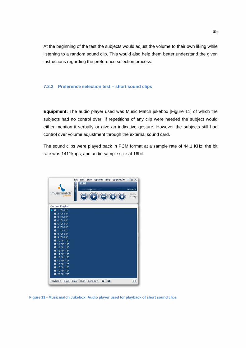
65

At the beginning of the test the subjects would adjust the volume to their own liking while

listening to a random sound clip. This would also help them better understand the given

instructions regarding the preference selection process.

7.2.2 Preference selection test – short sound clips

Equipment: The audio player used was Music Match jukebox [Figure 11] of which the

subjects had no control over. If repetitions of any clip were needed the subject would

either mention it verbally or give an indicative gesture. However the subjects still had

control over volume adjustment through the external sound card.

The sound clips were played back in PCM format at a sample rate of 44.1 KHz; the bit

rate was 1411kbps; and audio sample size at 16bit.

Figure 11 - Musicmatch Jukebox: Audio player used for playback of short sound clips

66

Procedure: The first part of the test to be conducted was a preference selection test of

short sound clips. The tests consist of matching segments from each of the two complete

mastered songs. They include as many different combinations of sounds in the song as

possible. [See section 7.1.1 for list of sound clips used].

Two of the same excerpts, one in stereo and one in 3D, are played after each other in a

random starting order with as many repetitions as the subject requested. The stereo and

3D sound versions were presented in a random order to avoid order effects. The subject

would then be asked to indicate one of the two sound clips he or she prefers. An

additional phrase states that the subject should select the sound clip that “sounds more

pleasant”. No further instructions regarding the basis for preference selection was given.

However, short discussions were sometimes necessary for the subject to understand

what exactly was required.

The total number of sound clips presented to the 35 subjects in the short sound clips

preference selection test was 1260 with an additional 140 clips being mocks. Selection

was done by writing either “1” if the first version was preferred and “2” if the second

version was preferred in the table provided. All repetitions to each sound clip were

recorded separately by the test administrator.

Subjects were not informed about the existence of the mock sound clips. Neither were

they informed that each repetition needed for the sound clips was being recorded. This

was done to avoid the possibility of subjects feeling the need to “impress” by having

good listening skills and not needing repetitions.

After a preference had been stated for each of the 20 excerpts (called Test A), the same

test was repeated but in a reversed order for both the sound clip pairs and the 3D/ stereo

presentation order (Test B). The subjects were informed that the test would be repeated

and that the order of sound clips would be altered.

7.2.3 Preference selection test – full song

A second listening test was performed after completing the first preference selection test.

The test involved listening to the full versions of the two songs and stating a preference

by selecting either version-01 or version-02. An option of stating “no preference” was

67

also available. Subjects were allowed to listen to the songs for as long as they chose to

and to restart it as often as they wanted.

The subjects were given control over the sequencer used for playback in order to switch

between the two versions at their own will and as often as they liked. This was done by

pressing either the up or down arrows on the keyboard on the portable computer. The

sequencer [Figure 12] allowed for seamless shifts between the two versions so the

subject could hear the differences between the versions in real-time. The first version to

be played was selected randomly to avoid a possible order effect.

Figure 12 - Nuendo sequencer used for playback in full song test

7.2.4 Additional questions

Besides completing the listening tests the subjects answered a number of questions

relating to the spatial attributes of the two versions and were able to express their views

on the spatial components of music in general. The perceived sound quality of the two

versions is also considered here. This part of the test was conducted as an informal

interview where each question was discussed to ensure it was understood correctly. The

questions are in a multiple choice format except for one question which is an open

question, also used also as a platform for further discussions. The structure of the

questions is based on results, conclusions and discussions from the pilot tests.

68

The questions covered a range of topics including more personal matters such as the

subject’s age, gender and how much music they listen to daily. Also subjects’ music

listening habits and preferences in general are covered in this section of the

questionnaire.

Other questions inquired directly about matters relating to the listening tests such as the

difficulty level in differentiating between the sound clips and the differences that made a

subject choose a particular sound clip/version over the other. One other question asks

whether the subjects perceived any sounds as coming from beyond the headphones.

69

8 Test results

Most subjects found the listening tests very interesting and would ask many questions

after completion. They seemed to have strong opinions and ideas to support their

preferences in choosing a particular version over the other. None of the participants had

ever heard of the term psychoacoustics before. Few had heard about the notion of 3

dimensional sound but none had heard about 3 dimensional sound produced with the

use of headphones.

The test results below are divided up into 3 groups in the same manner as the tests

section: short sound clips, full song, and extra questions.

8.1 Preference selection test results – short sound clips

Inconsistencies in Preference Selection: The results from the collected data varied a

great deal and also showed inconsistency between different subjects as well as

inconsistencies in the preferences from the subjects themselves. To obtain conclusive

results it was required that a subject would be more consistent in preferring one version

of the sound clips, and a considerable majority choosing the same version. But the

results indicate that the subjects had a tendency to change their preference very often

within the duration of the test, even for sound clips that were relatively easy to

distinguish apart.

On average a subject would select the same version of a sound clip (either stereo of 3D

sound) in the first and second tests only about half of the time (51%). The highest

consistency for a single subject choosing the same version was 16:18 (89%) and the

lowest was 5:18 (28%). The total number of repetitions for each sound clip was taken as

a measure of average level of difficulty for that specific clip. The inconsistencies could

not have been caused by the sound clips being too hard to tell apart from each other;

this is indicated in the additional questionnaire where subjects rated the difficulty levels

[Figure 20] and by the relative low number of repetitions needed for each sound clip.

70

Number of listening repetitions per sound clip: The data indicates the subjects were

fairly quick to make a decision regarding their preferences. A total of only 431 extra

repetitions were needed for all 1400 sound clips including the mock excerpts which in

fact sound the same (i.e. 3 repetitions for every 10 sound clips). The highest total

number of repetitions needed for a particular sound clip was 57 and the lowest was 10.

In fact the highest number of repetitions was not for a mock sound clip although this had

been the predetermined outcome. The most probable explanation to the high number of

repetitions for this clip is that it was the shortest of all sound clips (1.9 seconds). This

situation had on the other hand not showed up in the pilot test and could therefore not

have been corrected. The total number of repetitions for the two mock sound clips was

42 and 35 each. [See appendix 5 for preference selection results table].

Chi Square Test: The ratio of preferred sound clips for this test in the order “3D sound”

to “Stereo” was 660:600. From a face value analysis there was no conclusive trend in

the preference selection of the sound clips. A Chi-square test (X^2=2.857, df=1, p<0.05)

showed no significant preference of 3D sound as compared to stereo [Figure 13]. By

conventional criteria, this difference is considered to be not quite statistically significant.

Figure 13 - Chi square test graph for sound clips

71

Biases in Preference Selection: The test subjects could only choose between selecting

the first clip or the second clip in a pair by writing “1” or “2”. There were equally many

stereo and 3D sound clips assigned to play first in both tests. Statistically the ratio

between “1”s and “2”s should be equal if subjects were to randomly write a number. The

ratio for all sound clips in the order “1”:”2” was 783:617 [Figure 14].

However, it appeared that when subjects were uncertain of which version they preferred,

they would more often choose the first clip in a pair. This appeared to be more common

with the mock excerpts. The first sound clips in mock excerpts were selected about twice

as often as the second sound clips at a ratio of 93:47 [Figure 15].

Sound clips that were difficult to differentiate also showed a higher count for selected

first sound clips than the sound clips that were easy to differentiate. The median value

from the number of repetitions per sound clip was taken as a measure to define the

sound clip categories “difficult” and “easy”. In all 10 of the sound clips were defined as

easy and 10 were defined as difficult; these also included the mock excerpts. The ratio

for the difficult sound clips was 424:250 [Figure 16].

This pattern did however not reflect in the rest of the sound clips which were easier to tell

apart (clips with a low number of repetitions). Instead the distribution of “1’s” and “2’s”

was fairly equal at a ratio of 359:341 [Figure 17].

The tendency to choose the first sound clip also for mock excerpts indicates a certain

bias that might have an effect of the test results. A possible explanation for this tendency

could be that the listeners chose the “safest” option as was seen with the option of

choosing “no preference” in the pilot tests. The safest option in the case where both

sound clips are identical could be to choose the more familiar version; that is the version

they heard first and believe to be more familiar. The effect of this tendency is a subject

that will have to be investigated further for any conclusive justification of any bias.

72

Figure 14 – Selection rate of 1’s and 2’s for all sound clips

Figure 15 – Selection rate of 1’s and 2’s for mock sound clips

Figure 16 – Selection rate of 1’s and 2’s for difficult sound clips

Figure 17 – Selection rate of 1’s and 2’s for easy sound clips

0 500 1000Selection rate of "all" sound clips

"1"

"2"

0 50 100Selection rate of "mock" sound clips

"1"

"2"

0 200 400 600Selection rate of "difficult" sound clips

"1"

"2"

0 100 200 300 400Selection rate of "easy" sound clips

"1"

"2"

73

Learning effects: A possible trend that showed up is the increasing number of 3D

sound clips selected as the test progressed. In the first test the overall preference rating

showed the number of preferred 3D sound to stereo was equal at a ratio of 9:9. In the

second test however, the preference of 3D sound clips increased to a ratio of 12:6 with

the highest difference being with the last sound clips of the test. As mentioned in section

7.2.2, the playback order of sound clips was reversed in the second test, meaning the

sound clips played first (in Test A) were also the last ones in the second test (Test B). So

although a majority preferred the stereo clips at the beginning of the test, the 3D version

of the same clips were preferred towards the end of the test.

In [Figure 18], Graph 1 illustrates the overall trend in selection of 3D sound compared to

stereo for all sound clips (excluding mock sound clips). Graph 2 shows the first 5 sound

clips played in Test A and the last 5 sound clips to be played in Test B. These are in fact

the same sound clips as the order was reversed in the second test (Test B). It must be

pointed out that due to the low correlation coefficient values further research will have to

be undertaken before any meaningful conclusions can be made regarding this possible

trend.

Figure 18 – Graphs indicating an increasing preference for 3D sound clips as the test progresses

X-axis shows the chronological order in which the sound clips were played back. Y-axis shows the ratio between 3D sound and Stereo.

y = 0.0171x + 0.9522R² = 0.07

0.0

0.5

1.0

1.5

2.0

2.5

3.0

3.5

4.0

0 10 20 30 40

Rati

o of

3D

sou

nd /

Ste

reo

Presentation order of clips

Graph 1: 3D sound preference(All sound clips excluding mocks)

3D sound clips

Linear (3D sound clips)

y = 0.22x + 0.14R² = 0.4328

0.0

0.5

1.0

1.5

2.0

2.5

3.0

3.5

4.0

0 5 10 15

Rati

o of

3D

sou

nd :

Ster

eo

Presentation order of clips

Graph 2: 3D sound preference (5 first and 5 last clips)

3D sound clips

Linear (3D sound clips)

74

Salient Attributes influencing Preference Selection: Part of the aim of using short

sound clips was to underline individual attributes (instruments, vocals, spatial attributes

etc) in each of the sound clips which could possibly be preferred by a majority of

subjects. The evaluation is based on a face value analysis.

By analyzing the lead sounds in these excerpts, a general observation is that the 3D

effects were favored when used with 2 or more vocals while musical instruments were

favored in stereo. For example sound clips containing a chorus seemed to be preferred

as 3D sound compared to stereo most of the time. Only 3 sound clips stood out

particularly as being preferred by the majority of listeners. These are clips number 2, 3

and 20.

Clip number 2 contains a duet with the vocals as the lead sound. The 3D version of the

sound clip was selected 48 times as the preferred version, stereo was selected 22 times

out of a possible 70. Besides a wider acoustic field in the 3D version of this particular

sound clip, the vocals also appeared clearer. Clip number 20 was also preferred by a

majority as 3D sound at a ratio of 46:24. The lead sound in this clip was backup vocals in

a verse. Sound clip number 3 stood out with a majority preferring it as stereo at a ratio of

45:25. It was part of the intro section and contained an acoustic guitar and percussion

instruments as the lead sounds. More accurate basis for subjects’ choices will have to

include elicitation about individual sounds not only general feedback.

8.2 Preference selection test results – full song

General observations: In this test each subject would listen to the two versions for an

average of about 1.5 minutes, usually making a decision already after less than 1

minute. No repetitions were needed at any point. No subject selected “No preference” as

their response to which version they preferred.

Chi Square Test: Unlike the short sound clips, an obvious trend was visible for

preference ratings of the full song. The data showed a ratio of 25:10 of the subjects in

favor of stereo. A Chi-square test (X^2=6.429, df=1, p<0.05) showed significant

75

preference of stereo as compared to 3D sound [Figure 19]. By conventional criteria, this

difference is considered to be statistically significant.

Figure 19 - Chi square test graph for full song

Inconsistencies: Although the majority of listeners in this test considered the stereo

version to sound more pleasant, this was not necessarily reflected in their choice of

shorter sound clips. In the short sound clips test a total of 20 subjects favored 3D sound

clips in general as opposed to 10 in the full song test.

The shift from choosing 3D sound to choosing stereo was even visible with a number of

subjects who showed relatively high inclination in choosing 3D sound clips in the short

sound clips test. But contrary to the short sound clips test, subjects seemed much more

confident in their choice involving the full songs. This was partly indicated by the short

time needed to make a decision, usually less than 1 minute. Also, undocumented

repetitions of this test showed that subjects would choose the same version repeatedly

even after longer brakes between listening.

76

8.3 Additional questions

General observations: The interpretation of the data assisted in providing valuable

insight into this experiment. It also helped elaborate on some of the attributes and

motives that amount to preference of musical elements.

The additional questions indicated that neither age, gender nor the time spent daily

listening to music had any considerable impact on the overall results of the tests.

Many subjects struggled with finding own words to describe what it is they perceived. In

such a case non-leading questions and discussions helped subjects to formulate their

expressions easier.

Difficulty level in distinguishing between the two versions: One question in the test

inquired about the level of difficulty in distinguishing between the sound clips. It was

specifically directed at the short sound clips therefore the question had to be answered

before listening to the full song. Subjects provided answers on a 5 point scale ranging

from “very difficult” to “very easy” [Figure 20]. Before writing down their ratings subjects

would be informed about the mock excerpts that were included. With this extra

information the subjects had the option of changing their difficulty ratings. The majority

chose to keep their original ratings.

Subjects had varying opinions on the level of difficulty in differentiating between the two

presented versions; an overall assessment is that it was slightly difficult. However,

because the validity of individual assessments needs to be respected, these results

should as well be interpreted on a subject-to-subject basis rather than only given an

overall score. But even on a subject-to-subject basis the data did not reveal noticeable

correlation between the level of difficulty and a particular preference tendency.

77

Figure 20 - Level of difficulty in distinguishing between short sound clips

Sound Externalization: One particular area of interest was whether any sounds were

perceived by the subjects as externalized. Subjects were asked whether they thought

that any of the sounds from the stimuli appeared to come from beyond the physical limits

of the headphones. The aim with the question was to get a different perspective into the

relationship between the perceived width of the acoustic field and the preference ratings.

From the results it was observable the majority of subjects perceived sounds as coming

from beyond the headphones [Figure 21]. Through discussions with the subjects it

appeared that externalized sound was perceived only in the 3D versions.

As previously mentioned, the data does not suggest any prominent association between

the perceived width of the acoustic field and the preference ratings. Subjects with a

significant inclination to choosing 3D sound would regularly indicate not perceiving any

sound coming from beyond the headphones. Likewise, subjects with a high inclination to

choosing stereo would often perceive a wider sound image in the 3D sound version.

Despite noticing the aspect of externalized sound, the subjects would conversely prefer

stereo to 3D sound; meaning that in their case the deciding factors influencing

preference selection were other than only a wider acoustic field.

0 5 10 15Number of subjects

very easy

easy

moderate

difficult

very difficult

78

Figure 21 – Chart indicating whether subjects perceive sound as coming from beyond headphones

Hard Panning in 3D versions: Numerous remarks were made about the percussion

instruments in the 3D version being heard in only one ear. Because of this, prolonged

listening induced fatigue to the ipsilateral ear. Similar comments were also made about

the acoustic guitar in the 3D sound version. This problem was not observed in previous

informal localization tests in which the instruments were soloed. The percussion

instruments were in fact the easiest sounds to localize accurately as they were recorded

using a dummy-head which exhibited rather accurate localization. The problem of hard-

panned sounds was also absent when the instruments were soloed.

Feedback from subjects regarding spatial attributes: More data was collected from

the open questions and discussion sessions, mostly in regards to the differences

between the two versions and the reasons for the subjects’ choices. [Table 2] below

outlines some of the main points of the discussions from a number of selected

interviews. Mostly topics relating to the spatial dimensions of the two versions are

considered here although the discussed topics covered a much wider range.

A noticeable point is that no negative feedback was given to stereo. There are also a

number of conflicting points such as “clarity” and how “full” the song sounds. This can

partly be because the exact definitions of the terms used were not discussed prior to the

tests and also due to the fact that people perceive sound differently.

0 5 10 15 20Number of subjects

very much

yes

don't know

no

not at all

79

3D sound Stereo

+ - + --Sounds fuller-Vocals are good-Easy to hear individual instrument-Guitars sound better-3 dimensional-Big choir-More depth-Surround sound-Realistic-More clarity-Sense of depth-Feeling of presence-More space around-More stereo

-Too much high end-Reverb is too high on guitars-Sounds very sharp-Some sounds come from only one ear-Sound seem to come from everywhere-Confusing-Hard-panning-Echoes-Annoying-Sounds like a demo-Exhausting-Over stimulating-Too much percussion

-Warmer sound-More bass-Smooth-Gentle to the ear-Clear vocals-Clear guitars-Subtle bass-More dense-Soft-Intimate-Tight-Mellow-Sounds fuller-Relaxing

Table 2 - Positive and negative aspects of 3D sound and Stereo according to subjects

80

9 General discussion, conclusions and future directions

9.1 General Discussion

Past and Present Research: Various previous studies have suggested a direct

correlation between sound quality in headphone reproduction and the utilization of a wider

acoustic field [2,3,5,12,14,51]. Other studies have also shown similar results but with spatial

attributes having less significant influence on the overall sound quality [4,62,63]. Most of the

research has been conducted with relatively few consecutive sounds reproduced at one

time; which is not the case when listening to contemporary music. Furthermore, different

literature has suggested that as long as sound quality evaluation involves any hedonic

judgments such as assessing pleasantness the results are bound to contain biases [6].

In the present research, a new way of achieving a wider acoustic field for headphone

music has been presented. The proposed method aims at correcting some of the

problems encountered in previous attempts such as excessive coloration and other tonal

changes which are a result of post processing 3D algorithms. To measure the validity of

the proposed methods in experimental settings, a piece of music created with a wider

acoustic field was compared to a corresponding stereo version, which served as the

reference context. Additional interviews were conducted to obtain a better understanding

of the subjects’ preferences.

Answering the Research Question: Does a wider acoustic field in headphones enhance the quality of music?

The present research has not yielded any clear answers to whether listeners find a wider

acoustic field more pleasant. The research shows conflicting results to the notion that a

larger acoustic field enhances sound quality in headphones. However, the general trend

indicates that there is greater number of listeners who prefer regular stereo music. This

fact is underlined by the full song tests. Although it may be argued that the short sound

clips test showed a majority preferring the 3D sound, this test perhaps excludes the

important aspect in music listening which is interest [See section 4.2 What is music?].

Therefore it seems logical to put more credibility into the full song tests.

81

Despite a higher preference rating for stereo it has become clearer that the individualism

of listeners, past experiences as well as learning effects contribute to a large extent to

ratings of acoustic stimuli. These factors are very likely to be able to influence the

perceived sound quality and so must be taken into account for any reliable conclusions.

Learning effects: Listening experiments such as this one are usually designed to avoid

the learning effect as it may cause biases in the results. Despite measures taken in order

to avoid this situation test results have indicated a possible learning effect. Selection of 3D

sound version clips showed significant increase as the test progressed [Figure 18].

Nonetheless this does not have to be interpreted as a negative outcome. From these

results a positive relationship can be traced between subjects perceiving externalized

headphone sound and adapting to this new way of listening. It can be argued that

because there was equally much stereo stimulus presented, listeners could as well have

increased their preference for stereo instead of 3D sound.

Hard Panning of instruments in 3D sound version: The most probable explanation to

this problem is the effect of sound masking as previously discussed in section 2.4. There

was in fact no point at which the signal from a percussion instrument was panned to only

one channel during the whole production stage. At most the overall difference would be

about 8-15dB between the two channels.

Listeners instead perceived hard panning as a result of the weaker sound to the contra

lateral ear becoming masked by other sounds resulting in distortion of the IID levels and

probable simultaneous masking (the point when the weaker sound becomes inaudible).

From interviews with the listeners it appears that the perceived hard panning occurs

mostly in sections of the song with the most instruments, namely sections 3 and 5 [See

Figure 5].

Masking of salient localization cues seems to be a setback in this thesis because of the

large number of consecutive sounds. To some extent this matter may have affected

preference ratings as the subjects who made comments regarding hard panned sounds

eventually showed a preference for stereo. But even by eliminating these problems

through further tweaking it is still not certain that the listeners will necessarily prefer

externalized music compared to stereo.

82

9.2 Conclusions

Four main points will be presented as a result of an analysis of the collected test data and

earlier literature research:

Listeners’ preferences are not necessarily homogenous: The resultant data from the

tests shows a large variation in preferences with a multimodal distribution of scores,

suggesting that there may not be a key audio “format” preferred by the majority. The large

variations could be caused by listeners perceiving different attributes to be the important

contributors to the overall sound quality. Affective judgments are usually not homogenous

and so what one person likes may be disliked by another. The test involving the full song

preference selection shows clearly that although the majority preferred regular stereo, the

subjects who preferred the 3D version had strong valid arguments for doing so.

Listeners can change their mind regarding preferences: The data from the sound

clips test shows a very high rate of alternating preferences within the same test despite

subjects being relatively certain about their choices each time. The reason for the

alternating preferences is most likely explained by the biases that occur with any hedonic

judgments; these can lead to subjects changing their mind from influences such as mood

and situational contexts [6]. The encountered biases could have been reduced by focusing

on specific features of the sound such as only timbre or precise spatial attributes, but

because of the multidimensional nature of music it makes sense to conduct the research

by taking into account all possible perceptual aspects.

Listeners have expectations: Recently sound quality was defined as “the result of an

assessment of the perceived auditory nature of a sound with respect to its desired nature”

[57]. Stereo has been the standard for nearly all recorded music for the last couple of

generations and people have become accustomed to the format. This is perhaps seen to

some extent in the interviews whereby subjects did not have any negative comments

about the stereo version. Instead stereo may have been seen as the reference context

from which faults or improvements could be detected in the 3D version.

83

Listeners adapt: The present results show that when using headphones, the majority of

the population sample found regular stereo music more pleasant to listen to than music

with a wider acoustic field. The data also indicates that previous exposure to the stereo

format almost certainly causes certain expectations to what music should sound like, and

as a consequence influences preference ratings. Hearing is a dynamic process that

adapts easily to assimilate with the perceived sound, so although listeners have

preferences and expectations, these are prone to change with circumstances. [Figure 18]

shows a possible situation of subjects adapting to a new way of listening. It is possible

that if exposed to it over time, a clear majority could prefer a wider acoustic field when

listening to headphone music.

9.3 Future research

Improvements To Current Research: The present results show that the differences

between the two presented audio versions were in many cases not large enough to initiate

an absolute preference selection. A more radical approach in expanding the acoustic field

may yield results with fewer alterations in preference selection tests. Certain flaws such as

perceived hard panned sounds that appeared in stimuli will also have to be rectified for

any future research to achieve more conclusive results. It might also be essential to

establish a specific level from which spatial audio quality can be evaluated besides a

general preference test. The types of stimuli can also be increased to contain a larger

variety of music genres to fit a greater range of subjects.

Future Directions: There are many studies suggesting better “sound quality” with a larger

acoustic field in headphones, at least in laboratory settings which may not involve sounds

of a complex multidimensional nature. More research should be conducted into ways of

utilizing the benefits of technologies such as psychoacoustics which are a key to creating

wider acoustic fields for headphones.

As a result of this project, the most interesting inspiration is that listeners could probably

be influenced in a relative short time to change their preferences regarding perceived

sound quality. Research into this subject will allow more insight into how much of our

preferences are based on knowledge gained from exposure to the standard audio formats

84

and how much is spontaneous or reasoned. Perhaps by giving more exposure to new

audio formats it will allow listeners to learn a new way of listening in a 3 dimensional

space, thus opening up new exciting possibilities in soundscape design.

85

10 References

1 Owsinski Bobby (1990). “The Mastering Engineers Handbook. “

236 Georgia St. Suite 100 Vallejo, Ca. Auburn Hills, Mi.

2 Begault Durand R (1990). “The Composition of Auditory Space: Recent Developments in

Headphone Music.” Isast Pergamon Press Plc. Great Britain.

3 Liitola Toni. (2006). “Headphone Sound Externalization”. Helsinki University Of Technology.

Department Of Electrical And Communications Engineering Laboratory Of Acoustics And Audio

Signal Processing. Tampere, Finland

4 Fontana Simone, Farina Angelo, Greiner Yves (2007). “Binaural For Popular Music: A Case

Study.” Proceedings Of The 13th International Conference on Auditory Display, Montreal, Canada

5 Griesinger David (1990). “Binaural Techniques for Music Reproduction.” The Sound Of Audio:

Perception, And Measurement, Recording And Reproduction. 8th International Conference New

York. Audio Engineering Society.

6 Slawomir Zielinski (2006). “On Some Biases Encountered in Modern Listening Tests.” Institute Of

Sound Recording, University Of Surrey, Guildfor, Gu2 7xh, Uk.

7 Rumsey Francis (2001). “Spatial Audio.”

Published By Focal Press.

8 Am3d. Diesel Studios (2008). Http://Www.Am3d.Com/Products/Products?Headmenuid

=7bf455bf-0e44-4b01-83eb-A17145b14c1d&Menuid=7bf455bf-0e44-4b01-83eb-A17145b14c1d

(Retrieved 05.11.08)

9 Gaver William W (1993). “What In The World Do We Hear?: An Ecological Approach To Auditory

Event Perception.” Ecological Psychology. Lawrence Erlbaum Associates, Inc. Rank Xerox

Europarc, 61 Regent Street, Cambridge Cb2 Iab, England.

86

10 Zahorik Pavel (2002). “Auditory Display Of Sound Source Distance”. Proceedings Of The 2002

International Conference Onauditory Display, Kyoto, Japan. July 2-5, 2002.

Waisman Center, University Of Wisconsin - Madison

11 Pulkki V, Karjalainen M, Huopaniemi J (2001). “Analyzing Virtual Sound Sources Using A

Binaural Auditory Model.” Journal Of The Audio Engineering Society, 49(9): 739-752, November

2001.

12 Gardner William G (1999). “3d Audio And Acoustic Environment Modelling”. Wave Arts In. 99

Massachusetts Avenue, Suite 7 Arlington, Ma 02474. March 15, 1999

13 Shinn-Cunningham Barbara. “Learning Reverberation: Considerations For Spatial Auditory

Displays”. Dept. of Cognitive and Neural Systems and Biomedical Engineering. Boston

University.

14 Begault Durand R (2000). “3d Sound For Virtual Reality And Multimedia”

Ames Research Center, Moffet Field, California.

15 Hartman William M (1997). “How We Localize Sound. Extracts From The Text Book Signal,

Sound And Sensation”. Michigan State University, East Lansing, Michigan

16 Bakerd Brad, Hartmann William M . “Localization of Noise in a Reverberant Environment.”

Department Of Audiology And Speech Sciences,Michigan State University, East Lansing,

Mi, 48824, USA

17 Gardner William G (1999). “3d Audio and Acoustic Environment Modelling”. Wave Arts In. 99

Massachusetts Avenue, Suite 7 Arlington, Ma 02474. March 15, 1999

18 Shinn-Cunningham Barbara. “Learning Reverberation: Considerations For Spatial Auditory

Displays”. Dept. Of Cognitive And Neural Systems And Biomedical Engineering. Boston

University.

19 Griesinger David (1990). “Binaural Techniques for Music Reproduction”. The Sound Of Audio:

Perception, and Measurement, Recording And Reproduction. 8th International Conference New

York. Audio Engineering Society 1990.

87

20 Owsinski Bobby, O’brien Malcolm (1999). “The Mixing Engineers Handbook.”

236 Georgia St. Suite 100 Vallejo, Ca. Auburn Hills, Mi. 1999

21 Franz David (2004). “Recording and Producing in the Home Studio”. A Complete Guide.

Berklee Press, 1140 Boylston Street Boston, Ma 02215 USA. 2004

22 Audio Design Line (2009). Http://www.audiodesignline.com/ (Retrieved 11.02.09)

23 Algazi V. R, Duda R. O, Avendano C. And Thompson D. M (2001). “The Cipic Hrtf Database.”

ieee Workshop on Applications of Signal Processing to Audio and Acoustics 2001

24 Blauert Jens, Allen John S (1997). “Spatial Hearing: The Psychophysics Of Human Sound

Localization.” Mit Press, 1997.

25 Science World. Wolfram Research (2008).Http://Scienceworld.Wolfram.Com/Physics/

Dopplereffect.html (Retrieved On 10.10.08)

26 Chowning John M (2000). “Digital Sound Synthesis, Acoustics, And Perception: A Rich

Intersection”.Proceedings of the Cost G-6 Conference On Digital Audio Effects (Dafx-00), Verona,

Italy, December 7-9, 2000

Duda Richard O (2008). “Principles Of 3d Audio.” Department Of Electrical Engineering, San

Jose State University. Http://Www.Audiodesignline.Com/ (Retrieved 11.02.09)

28 Jack C. E. and Thurlow W. R (1973). “Effects Of Degree Of Visual Association And Angle Of

Displacement on the "Ventriloquism" Effect,” Percept. Mot. Skills, Vol. 37, 1973

Kashino Kuino. Hidehiko Tanaka (1993). “A Sound Source Separation System with the Ability of

Automatic Tone Modeling”. Department Of Electrical Engineering, Faculty Of Engineering. The

University Of Tokyo.

30 Lorenzi Christian, Gatehouse Stuart, Lever Catherine (1999). “ Sound Localization in Noise in

Normal Hearing Listeners”. The Journal Of The Acoustical Society Of America -- March 1999 --

Volume 105.

31 Wiklander Roger (2001). Nuendo Dts Encoder. Operation Manual.

Steinberg Media Technologies Gmbh, 2004. P 15

88

32 Guastavino Catherine, archerVéronique L, Guillaume Catusseau and Patrick Boussard (2007). “Spatial Audio Quality Evaluation: Comparing Transaural, Ambisonics and Stereo”. Proceedings

of the 13th International Conference on Auditory Display, Montréal, Canada, June 26-29, 2007

33 Pulkki Ville (2001). “Spatial Sound Generation And Perception By Amplitude Panning

Techniques”. Helsinki University of Technology Laboratory of Acoustics and Audio Signal

Processing. Espoo 2001.

34 Sneegas James E (1987). “Aural Acuity and the Meaning of Sound Quality: A Cultural Approach”.

Aes 83rd Convention. New York, N.Y. 1987

35 Spors Sasha, abensteinRudolf R, and AhrenJens s (2008). “The Theory Of Wave Field Synthesis

Revisited”. Audio Engineering Society. Presented At The 124th Convention. 2008 May 17–20

Amsterdam, The Netherlands

36 Theile Günther (2004). “Wave Field Synthesis – A Promising Spatial Audio Rendering Concept.”

Proc. of the Int. Conference on Digital Audio Effects (Dafx-04), Naples, Italy, October 5-8, 2004.

37 Malham D (2003). “Higher Order Ambisonic Systems”. Abstract From “Space In Music - Music In

Space”, University Of York In April 2003

38 Malham D. ”Experience With Large 3-D Ambisonics Sound Systems”. Music

Technology Group, Department of Music, University of York, Heslington, York.

39 Pulkki Ville, Lokki Tapio. ” Creating Auditory Displays With Multiple Loudspeakers Using VBAP”.

Laboratory Of Acoustics And Audio Signal Processing, Helsinki University Of Technology.

40 Ville Pulkki (1999). “Uniform Spreading Of Amplitude Panned Virtual Sources”. Proc. 1999 ieee

Workshop on Applications Of Signal Processing To Audio And Acoustics, New Paltz, New York,

Oct. 17-20, 1999

41 Pulkki Ville, Karjalainen Matti (2001). “Directional Quality Of 3-D Amplitude Panned Virtual

Sources”. Proceedings Of The 2001 International Conference On Auditory Display, Espoo,

Finland, July 29-August 1, 2001

89

42 Pulkki V. and Karjalainen M (2001). “Localization Of Amplitude-Panned Virtual Sources I:

Stereophonic Panning.” Jaes Volume 49 Issue 9 Pp. 739-752; September 2001

43 Jot J. M, Larcher, V. And J. M. Pernaux (1999). “A Comparative Study Of 3d Audio Encoding And

Rendering Techniques”. In Proc. Aes 16th International Conference on Spatial Sound

Reproduction. Rovaniemi Finland. April 1999

44 Leakey D M (1959). “Some Measurements On The Effect Of Inter-Channel Intensity And Time

Difference in Two Channel Systems”. J. Acoustic Society Am. Vol 31. 1959

45 Bauer B.B (1961). ”Phasor Analysis Of Some Stereophonic Phenomena”.

J. Acoustic Society. Am. Vol. 33. November 1961

46 Shepherd Ashley and Gue´Rin Robert (2004). “Nuendo Power!”. Thomson Course Technology

Ptr. 25 Thomson Plave Boston, M A 02210

47 Ward, D.B. Elko, G.W (2002). “Effect Of Loudspeaker Position On The Robustness Of Acoustic

Crosstalk Cancellation” Acoust. & Speech Res. Dept., Lucent Technol., Murray Hill, Nj; 2002

48 Wenzel Elizabeth M, Arruda Marianne. Frederic Wightman (1993). “Localization Using

Non-individualized Head-Related Transfer Functions.” J. Acoust. Soc. Am. 94(1). July 1993

49 H. Møller (1992), “Fundamentals Of Binaural Technology,” Applied Acoustics, Volume 36, Issue

3-4, 1992.

50 Hartman W.M (1985). “Localization Of Sound In Rooms, Ii: The Effects Of A Single Reflecting

Surface”. Journal Of The Audio Engineering Society. 1985.

51 Farina Angelo . “An Example Of Adding Special Impression To Recorded Music: Signal

Convolution With Binaural Impulse Response.” Dipartimento Ingegneria Industriale

52 Shinn-Cunningham B.G (2000). “Distance Cues For Virtual Auditory Space.” Proceedings Of The

First ieee Pacific-Rim Conference On Multimedia, 13-15 December 2000 Sydney, Australia.

Boston University Hearing Research Center.

90

53 Martignon Paolo, Azzali Andrea, Cabrera Densil, Andrea Capra, and Farina Angelo (2005).

“Reproduction of Auditorium Spatial Impression with Binaural and Stereophonic Sound Systems.”

Audio Engineering Society. 118th Convention. 2005 May 28–31 Barcelona, Spain

54 Theile Günther (2001). “Multichannel Natural Music Recording Based On Psychoacousitc

Principles.” Extended Version Of The Paper Presented At The AES 19th International

Conference, May 2001 Irt D-80939 München, Germany

55 Letowski T (1989). “ Sound Quality Assessment: Concepts And Criteria,” AES 87th Convention,

October 13-21, New York, Paper 2825 (1989)

56 Blauert J, And Jekosh U (1997). “Sound Quality Evaluation – A Multi-Layered Problem,”

Acoustica United with Acta Acustica, Vol. 83 (1997)

57 Jekosch U (2004). “Basic Concepts And Terms Of ‘Quality’, Reconsidered in The Context of

Product-Sound Quality,” Acusitica United With Acta Acustica, Vol 90 (2004)

58 Pellegrini Renato S (2001). “Quality Assessment Of Auditory Virtual Environments” Proceedings

of the 2001 International Conference On Auditory Display, Espoo, Finland, July 29-August 1,

2001

59 Philip Alperson (1987). “What Is Music? An Introduction to the Philosophy Of Music.”

Haven Publications, California USA1987

60 Kostelanetz Richard (2003). “Conversing With John Cage”.

Routledge, 2003.

61 Standard Dictionary Definition

62 Rumsey Francis (2006). “Spatial Audio And Sensory Evaluation Techniques – Context, History

And Aims.” Institute Of Sound Recording, University Of Surrey, Guildford, Gu2 7xh, Uk

63 Rumsey Francis, Zielinski S, R. Kassier and Bechs S. “Relationships Between Experienced

Listener Ratings of Multichannel Audio Quality and Naïve Listening Preferences.”J. Acoust. Soc.

Amer.11764 Rumsey Francis and Berg jan. “Systematic Evaluations Of Perceived Spatial Quality.”

AES 24th International Conference on Multichannel Audio

91

65 Zacharov Nick and Koivumiemi Kalle (2001). “Audio Descriptive Analysis & Mapping Of Spatial

Sound Displays.” Proceedings Of The 2001 International Conference On Auditory Display,

Espoo, Finland, July 29-August 1, 2001

66 Zacharov Nick and Koivumiemi Kalle (2001). “Understanding Spatial Sound Reproduction:

Perception and Preference”. Proceedings Of The 2001 International Workshop On Spatial Media,

Aizu-Wakamatsu, Japan, Oct. 25-26, 2001

67 Delone (1975). “Aspects Of Twentieth-Century Music”.

Englewood Cliffs, New Jersey: Prentice-Hall 1975

68 Hotel Proforma (2008). Lecture by Brixen Eddy Bøgh.

http://www.ebb-consult.com/ Copenhagen.

69 Am3d. Product Overview.( Retrieved On 31.10.08)

http://www.am3d.com/Products/Products?Headmenuid=7bf455bf-0e44-4b01-83eb-

A17145b14c1d&Menuid=7bf455bf-0e44-4b01-83eb-A17145b14c1d

70 Am3d. Diesel Studios (2008). http://www.am3d.com/ Advanced Use - Tutorial 7

(Retrieved On 04.11.08)