
Enhancing Energy Efficiency in the ... - fis.uni-bamberg.de
19
University of Bamberg, Information Systems and Energy Efficient Systems Enhancing Energy Efficiency in the Residential Sector with Smart Meter Data Analytics* Konstantin Hopf, Mariya Sodenkamp, Thorsten Staake University of Bamberg Chair of Information Systems and Energy Efficient Systems D-96045 Bamberg Correspondence: [email protected], [email protected] *This is a post-peer-review, pre-copyedit version of an article published in Electronic Markets - The International Journal on Networked Business. The final authenticated version was accepted on February 6, 2018 and is published: http://dx.doi.org/ 10.1007/s12525-018-0290-9. Use the following citation to reference this article: Hopf, K., Sodenkamp, M. & Staake, T. Enhancing energy efficiency in the residential sector with smart meter data analytics. Electron Markets 28, 453–473 (2018) doi:10.1007/s12525-018-0290-9 Abstract Tailored energy efficiency campaigns that make use of household-specific information can trigger substantial energy savings in the residential sector. The information required for such campaigns, however, is often missing. We show that utility companies can extract that information from smart meter data using machine learning. We derive 133 features from smart meter and weather data and use the Random Forest classifier that allows us to recognize 19 household classes related to 11 household characteristics (e.g., electric heating, size of dwelling) with an accuracy of up to 95% (69% on average). The results indicate that even datasets with an hourly or daily resolution are sufficient to impute key household characteristics with decent accuracy and that data from different yearly seasons does not considerably influence the classification performance. Furthermore, we demonstrate that a small training data set consisting of only 200 households already reaches a good performance. Our work may serve as benchmark for upcoming, similar research on smart meter data and provide guidance for practitioners for estimating the efforts of implementing such analytics solutions. Keywords classification, decision support systems, data analytics, energy efficiency, sustainability, green information systems URN:urn:nbn:de:bvb:473-irb-470185 DOI: https://doi.org/10.20378/irb-47018
Transcript of Enhancing Energy Efficiency in the ... - fis.uni-bamberg.de
University of Bamberg, Information Systems and Energy Efficient Systems
Enhancing Energy Efficiency in the Residential Sector with Smart Meter Data Analytics*
Konstantin Hopf, Mariya Sodenkamp, Thorsten Staake
University of Bamberg Chair of Information Systems and Energy Efficient Systems
D-96045 Bamberg
Correspondence: [email protected], [email protected]
*This is a post-peer-review, pre-copyedit version of an article published in Electronic Markets - TheInternational Journal on Networked Business. The final authenticated version was accepted on
February 6, 2018 and is published: http://dx.doi.org/ 10.1007/s12525-018-0290-9.
Use the following citation to reference this article:
Hopf, K., Sodenkamp, M. & Staake, T. Enhancing energy efficiency in the residential sector with smart meter data analytics. Electron Markets 28, 453–473 (2018) doi:10.1007/s12525-018-0290-9
Abstract Tailored energy efficiency campaigns that make use of household-specific information can trigger substantial energy savings in the residential sector. The information required for such campaigns, however, is often missing. We show that utility companies can extract that information from smart meter data using machine learning. We derive 133 features from smart meter and weather data and use the Random Forest classifier that allows us to recognize 19 household classes related to 11 household characteristics (e.g., electric heating, size of dwelling) with an accuracy of up to 95% (69% on average). The results indicate that even datasets with an hourly or daily resolution are sufficient to impute key household characteristics with decent accuracy and that data from different yearly seasons does not considerably influence the classification performance. Furthermore, we demonstrate that a small training data set consisting of only 200 households already reaches a good performance. Our work may serve as benchmark for upcoming, similar research on smart meter data and provide guidance for practitioners for estimating the efforts of implementing such analytics solutions.
Keywords classification, decision support systems, data analytics, energy efficiency, sustainability, green information systems
URN:urn:nbn:de:bvb:473-irb-470185DOI: https://doi.org/10.20378/irb-47018
Smart Meter Data Analytics for Residential Energy Efficiency page 2/19
Introduction In their attempt to promote energy efficiency and the integration of renewable energy sources in the electric grid, policy makers have placed high hopes on networked electricity meters. The devices – often referred to as smart meters – collect consumption data of individual households and communicate the information to metering operators at time intervals of typically 15 minutes (European Commission, 2012). Smart meters facilitate billing processes, simplify the switch to another energy supplier for end-customers, enable dynamic tariff schemes to incentivize load shifting programs, and may induce energy conservation efforts by means of timely consumption feedback. In line with their strategies towards a sustainable and competitive electricity market, many countries have mandated utility companies to roll out the technology among their residential customers. So far, 16 of 27 EU member states decided for a “large-scale roll-out of smart electricity metering by 2020 or earlier” where more than 80% of conventional meters will be replaced (European Commission, 2014). The European Commission estimates that approximately 95 million meters will be deployed by 2020 (this is about 72% of all EU electricity consumers). In the U.S., more than 70 million smart meters have been installed by 2016 (U.S. Energy Information Administration, 2017).
The initial enthusiasm for the technology, however, has faded recently. Unlike early studies that rely on small convenience samples of motivated volunteers (Darby, 2006), most larger and more carefully designed recent pilot projects report savings of only around 3% and little response to incentives for load shifting (McKerracher & Torriti, 2013). Moreover, early technology-centric feedback campaigns together with inadequate data protection practices or missing information on data usage raised substantial privacy concerns among consumers (Buchanan, Banks, Preston, & Russo, 2016; McKenna, Richardson, & Thomson, 2012). It has become evident that relying merely on the plain communication of consumption data and price incentives are neither sufficient to advance energy literacy, nor motivate the hoped-for behavioral change, nor trigger investments in saving technologies (Graml, Loock, Baeriswyl, & Staake, 2011). This shortcoming is a major issue, because efficiency gains and more engaged consumers had been key reasons justifying the rollout of the costly infrastructure (Ecoplan, 2015).
Yet, several studies show that feedback information can successfully trigger meaningful energy savings if the information is tailored to the feedback receiver, for instance by using comparisons with similar households in the neighborhood (Allcott, 2011), by focusing on particular target behaviors (Tiefenbeck et al., 2016), or by providing suitable conservation goals (Loock, Staake, & Thiesse, 2013). Such household-
specific measures can yield lower costs per kWh saved than taxes and price increases, and can meet higher public acceptance than prohibitive regulations (Allcott & Mullainathan, 2010). However, specific interventions require rich information about the feedback receiver (Tiefenbeck, 2017), which metering operators and utility companies typically do not possess.
We argue that the necessary information can be extracted from available smart metering data and even with small training data sets, as the load shapes are the result of many stable household characteristics and behaviors. By means of supervised learning, we strive to uncover these characteristics and behaviors. The exemplifying analyses are based on a sample of 527 households in Switzerland. Feature vectors have been derived from smart meter data collected at 15-minute granularity over one week (7 days) and are augmented by weather data. For training and testing, survey data was available from each household. The household characteristics predicted (also referred to as properties hereafter) include household inventory data such as the type of water and space heating system, age of the building, and the number of electric appliances, among others, as well as preferences regarding the households’ interest in purchasing a rooftop photovoltaic system. Moreover, we investigate the effects of the temporal resolution of the consumption data on the accuracy of the results, provide an estimate of the necessary size of training data, and determine the seasonal impact of environmental conditions on the classification performance.
Our work contributes to the field of energy informatics (Watson, Boudreau, & Chen, 2010; Watson, Howells, & Boudreau, 2012): We outline how smart meters, which will be deployed in hundreds of millions of households worldwide in the near future, can deliver the information needed for targeted interventions to achieve the hoped-for savings effects. The article expands on recent research on household classification (Beckel, Sadamori, & Santini, 2013; Beckel, Sadamori, Staake, & Santini, 2014) and contributes to the large body of work in the information systems literature that aims at providing decision support for effective customer communication based on company-internal information and market data (Chang, Wong, & Fang, 2014; Zhang, Agarwal, & Lucas, 2011). Furthermore, our research informs the ongoing privacy debate regarding smart meter data as it highlights to what extent household characteristics can be revealed. For practitioners, the results may establish the missing link between available consumption data time series and effective, scalable energy efficiency measures.
Smart Meter Data Analytics for Residential Energy Efficiency page 3/19
Related Work Processing and managing customer data for a more effective customer communication has already been subject of early publications in the field of management information systems (Synnott, 1978). Since then, the field of database marketing (Lewington, De Chernatony, & Brown, 1996) and later customer relationship management systems (Chang et al., 2014; Coltman, 2007; Xu & Walton, 2005) has investigated how to create information systems that effectively impute and manage knowledge on individuals from data that is owned by companies. These customer insights can be exploited to realize personalization and ultimately increase sales – for instance with personalized product recommendations (Zhang et al., 2011) – or improve customer loyalty – for example by supporting post-purchase services or customer support (Otim & Grover, 2006). In an insightful contribution, Wattal et al. (2011) demonstrate that e-mail communication with customers is more effective when including relevant contextual information (e.g., on products or services that fit to them) compared with communication that is simply personalized with the recipients’ names. To make use of a rich communication and targeted recommendations, companies thus try to augment their customer data with relevant knowledge.
The growing availability of data and recent progress in data analytics provide a rich toolset to infer customer details in general (Constantiou & Kallinikos, 2015; Yoo, 2015). In the specific case of the utility industry, the deployment of smart meters makes fine-grained consumption data available to energy retailers and enables manifold possibilities to create value from such data (Ecoplan, 2015). The major challenge, however, is to make sense of the data streams and infer customer insights such as household characteristics, attitudes, or behavior that can support marketing departments or inform targeted energy efficiency campaigns.
Several researchers have developed methods to gather household characteristics from energy consumption data; approaches differ with respect to the type of data available (e.g., meter readings, household survey reports), their resolution in time (from multiple Hertz to annual electricity consumption) and the output variables of interest (saving potential, income, etc.). Obviously, the potential to recognize household characteristics from load curves depends on the data granularity – the higher the resolution in time, the better is the recognition performance that can be achieved.
Extensive research has been conducted to develop load monitoring techniques for recognizing electric appliances based on central measurement points providing data of high resolution in time (sampling frequencies typically in the range of kilohertz to
megahertz), called non-intrusive load monitoring (Birt et al., 2012; Hart, 1992). Although sampling rates far beyond one megahertz are common in industrial or lab settings, the smart metering infrastructure that is being deployed and that is expected to be in the field for the next 20 years does not provide such fine-grained data. Therefore, non-intrusive load monitoring approaches will most likely not be compatible with the standard meters deployed in most households (Armel, Gupta, Shrimali, & Albert, 2013; Kim, Marwah, Arlitt, Lyon, & Han, 2011).
Based on low time resolution consumption data with 15-minute to 60-minute reading intervals, several studies apply automatic unsupervised clustering techniques to identify customers with similar consumption patterns (Albert & Rajagopal, 2014; Al-Otaibi, Jin, Wilcox, & Flach, 2016; Beckel, Sadamori, & Santini, 2012; Chicco, 2012; de Silva, Xinghuo, Alahakoon, & Holmes, 2011; Flath, Nicolay, Conte, Dinther, & Filipova-Neumann, 2012; Kwac, Tan, Sintov, Flora, & Rajagopal, 2013; McLoughlin, Duffy, & Conlon, 2012). The resulting customer segments need further interpretation by experts before the insights can inform energy efficiency programs or marketing campaigns. Therefore, we focus on the recognition of energy efficiency characteristics using supervised machine learning algorithms, because the household-specific predictions can directly be used in respective campaigns. Recent works show that certain household characteristics can be inferred with good accuracy from electricity consumption data. Basic information about households with strong impact on overall electricity consumption such as household type, number of residents or presence of electric heating systems can be predicted based on annual consumption data and geographic information (Hopf, Riechel, Sodenkamp, & Staake, 2017; Hopf, Sodenkamp, & Kozlovskiy, 2016). The inference of more detailed household properties seems to require at least daily consumption measurements: heat pumps can be identified with daily electricity consumption data (Fei et al., 2013) and the existence of electric vehicles in households can be predicted based on hourly electricity consumption data (Verma, Asadi, Yang, & Tyagi, 2015). Based on 30-minute smart meter data from the U.S., Albert & Rajagopal (2013) apply Hidden Markov models to raw smart meter load curves to predict the existence of 10 household properties. The classification performance in their study is, however, low: the predicted existence of clothes dryers and washing machines is, for example, correct in only half of the cases; for other properties, the prediction error is even higher. Beckel et al. (2013, 2014) suggest reducing the raw load curve to a set of 35 features; they assess the performance of four classification algorithms in revealing 18 household properties. Among those properties, most relate to the inhabitants’ life situation (age, family, employment, social class, etc.), and three directly relate to energy efficiency (number of appliances, cooking type and

Smart Meter Data Analytics for Residential Energy Efficiency page 4/19
lightbulbs). The team achieved an average accuracy of 65% ranging from 39% to 82% with data from households in Ireland These results can be further improved by empirically defining 93 features and applying automatic feature selection (Hopf, Sodenkamp, Kozlovskiy, & Staake, 2014).
The work presented in this article expands previous studies by showing that a state-of-the-art machine learning algorithm (Random Forest) can be used to predict energy efficiency related household properties. We also examine the influence of the smart meter data resolution, the necessary number of households that must be available for training, and the seasonality on algorithm performance. Aside from adding more household characteristics to the list of recognizable properties, the study also allows to determine if the approach is also feasible for the large majority of relatively small utility companies that dominate many markets.
Research Objective To provide a common ground and ease the comparability of the results with related studies, we predict three energy efficiency related household properties that have been subject to earlier investigations (number of appliances, type of cooking facility, and age of residency). Moreover, we extend the list by eight new properties that can be revealed from smart meter data at 15-minute granularity (space heating type and age, water heating type, heat pump usage in a household, age of appliances, presence and interest in photovoltaic or solar heat installations, and number of recently completed energy efficiency measures). The prediction reflects the learnings from an earlier household classification study (Sodenkamp, Kozlovskiy, Hopf, & Staake, 2017) regarding various machine learning algorithms. Thus, our first research question (RQ) is:
RQ 1. How well can the aforementioned properties that are associated with high electricity consumption be recognized based on common smart meter data with a state-of-the-art standard method of machine learning?
Additional to the general ability to recognize household properties from electricity consumption data, we examine how marginal conditions related to data economy (i.e., data granularity and limited datasets) and environmental influences (i.e., seasonal impact) affect the performance of the predictive information system. More specifically, we investigate to what extent four important factors influence the quality of the classification:
Factor 1: Smart meter data resolution – The availability of detailed electricity consumption data traces to the utilities is associated with consumers’ privacy concerns (Buchanan et al., 2016; McKenna et al., 2012). Depending on the company policy and local
legislation, utilities make use of different data granularities. The typical aggregations vary between 15-minute, 30-minute, hourly and daily levels. For daily data, some utilities differentiate between the HT (high tariff, usually during the day) and NT (low tariff, usually during the night) consumption. Data with lower frequency contains less information about customers’ behavior and one can expect the performance of our classification algorithms to degrade when applied to such data. On the other hand, the performance of machine learning may be negatively affected by high data dimensionality if features are not selected carefully (Keogh & Mueen, 2011).
Factor 2: Number of weeks for algorithm training – An interval of energy consumption data may be affected by outliers. Therefore, household classification results that are based on single weeks of electricity consumption can be expected to be improved by making predictions based on multiple weeks of data, because this could also improve prediction models for energy demand (Li, Bowers, & Schnier, 2010). The magnitude of the improvements are therefore subject to our investigation.
Factor 3: Number of training instances – Furthermore, we investigate the impact of the number of training examples with known household characteristics (ground truth) on the accuracy of the household classification. This information is helpful for planning and conducting surveys, for example to gather data on new household information, or when the classification models need to be adapted to region-specific ground truth data for improved predictions.
Factor 4: Yearly season of training data – In this study, we show how to extract several season-specific household characteristics (e.g., space heating due to lower temperatures and increased occupancy during the winter). Therefore, we expect that the prediction accuracy for energy efficiency properties (i.e., space heating type, existence of a heat pump and the number of appliances) changes drastically based on the current week of the year used in classification, because these properties are strongly dependent on weather variables, such as outside temperature or sunshine hours per day.
The second RQ covers the above-mentioned factors:
RQ 2. How important is the temporal resolution of the smart meter data, what number of households must be available, and is it necessary to have data from different yearly seasons for algorithm training?
Answering these questions helps practitioners to estimate the cost of implementing appropriate analytics solutions and constitutes a benchmark for data experts and researchers to assess the quality of their solutions.
Smart Meter Data Analytics for Residential Energy Efficiency page 5/19
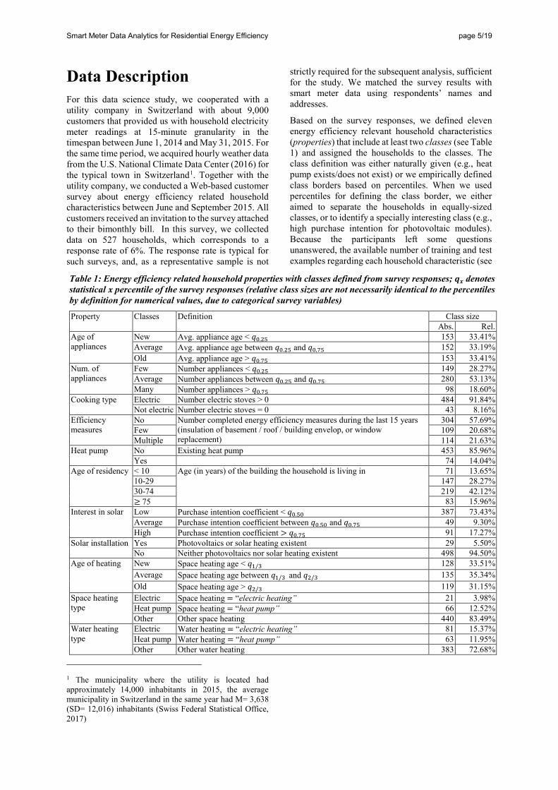
Data Description For this data science study, we cooperated with a utility company in Switzerland with about 9,000 customers that provided us with household electricity meter readings at 15-minute granularity in the timespan between June 1, 2014 and May 31, 2015. For the same time period, we acquired hourly weather data from the U.S. National Climate Data Center (2016) for the typical town in Switzerland1. Together with the utility company, we conducted a Web-based customer survey about energy efficiency related household characteristics between June and September 2015. All customers received an invitation to the survey attached to their bimonthly bill. In this survey, we collected data on 527 households, which corresponds to a response rate of 6%. The response rate is typical for such surveys, and, as a representative sample is not
1 The municipality where the utility is located had approximately 14,000 inhabitants in 2015, the average municipality in Switzerland in the same year had M= 3,638 (SD= 12,016) inhabitants (Swiss Federal Statistical Office, 2017)
strictly required for the subsequent analysis, sufficient for the study. We matched the survey results with smart meter data using respondents’ names and addresses.
Based on the survey responses, we defined eleven energy efficiency relevant household characteristics (properties) that include at least two classes (see Table 1) and assigned the households to the classes. The class definition was either naturally given (e.g., heat pump exists/does not exist) or we empirically defined class borders based on percentiles. When we used percentiles for defining the class border, we either aimed to separate the households in equally-sized classes, or to identify a specially interesting class (e.g., high purchase intention for photovoltaic modules). Because the participants left some questions unanswered, the available number of training and test examples regarding each household characteristic (see
Table 1: Energy efficiency related household properties with classes defined from survey responses; 𝒒𝒒𝒙𝒙 denotes statistical 𝒙𝒙 percentile of the survey responses (relative class sizes are not necessarily identical to the percentiles by definition for numerical values, due to categorical survey variables)
Property Classes Definition Class size Abs. Rel.
Age of appliances
New Avg. appliance age < 𝑞𝑞0.25 153 33.41% Average Avg. appliance age between 𝑞𝑞0.25 and 𝑞𝑞0,75 152 33.19% Old Avg. appliance age > 𝑞𝑞0.75 153 33.41%
Num. of appliances
Few Number appliances < 𝑞𝑞0.25 149 28.27% Average Number appliances between 𝑞𝑞0.25 and 𝑞𝑞0.75 280 53.13% Many Number appliances > 𝑞𝑞0.75 98 18.60%
Cooking type Electric Number electric stoves > 0 484 91.84% Not electric Number electric stoves = 0 43 8.16%
Efficiency measures
No Number completed energy efficiency measures during the last 15 years (insulation of basement / roof / building envelop, or window replacement)
304 57.69% Few 109 20.68% Multiple 114 21.63%
Heat pump No Existing heat pump 453 85.96% Yes
74 14.04%
Age of residency < 10 Age (in years) of the building the household is living in 71 13.65% 10-29 147 28.27% 30-74 219 42.12% ≥ 75 83 15.96%
Interest in solar Low Purchase intention coefficient < 𝑞𝑞0.50 387 73.43% Average Purchase intention coefficient between 𝑞𝑞0.50 and 𝑞𝑞0.75 49 9.30% High Purchase intention coefficient > 𝑞𝑞0.75 91 17.27%
Solar installation Yes Photovoltaics or solar heating existent 29 5.50% No Neither photovoltaics nor solar heating existent 498 94.50%
Age of heating New Space heating age < 𝑞𝑞1/3 128 33.51% Average Space heating age between 𝑞𝑞1/3 and 𝑞𝑞2/3 135 35.34% Old Space heating age > 𝑞𝑞2/3 119 31.15%
Space heating type
Electric Space heating = “electric heating” 21 3.98% Heat pump Space heating = “heat pump” 66 12.52% Other Other space heating 440 83.49%
Water heating type
Electric Water heating = “electric heating” 81 15.37% Heat pump Water heating = “heat pump” 63 11.95% Other Other water heating 383 72.68%
Smart Meter Data Analytics for Residential Energy Efficiency page 6/19
Table 1) does not necessarily sum up to the total number of survey responses. The percentage of unanswered questions is 23.91% for ‘age of residency’, 34.35% for ‘age of appliances’, 40% for ‘age of heating’, and 23.48 % for the remaining household properties.
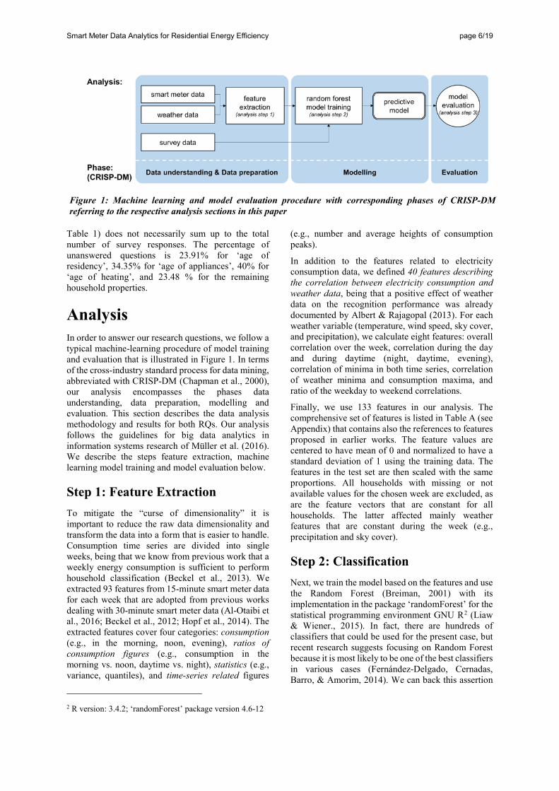
Analysis In order to answer our research questions, we follow a typical machine-learning procedure of model training and evaluation that is illustrated in Figure 1. In terms of the cross-industry standard process for data mining, abbreviated with CRISP-DM (Chapman et al., 2000), our analysis encompasses the phases data understanding, data preparation, modelling and evaluation. This section describes the data analysis methodology and results for both RQs. Our analysis follows the guidelines for big data analytics in information systems research of Müller et al. (2016). We describe the steps feature extraction, machine learning model training and model evaluation below.
Step 1: Feature Extraction To mitigate the “curse of dimensionality” it is important to reduce the raw data dimensionality and transform the data into a form that is easier to handle. Consumption time series are divided into single weeks, being that we know from previous work that a weekly energy consumption is sufficient to perform household classification (Beckel et al., 2013). We extracted 93 features from 15-minute smart meter data for each week that are adopted from previous works dealing with 30-minute smart meter data (Al-Otaibi et al., 2016; Beckel et al., 2012; Hopf et al., 2014). The extracted features cover four categories: consumption (e.g., in the morning, noon, evening), ratios of consumption figures (e.g., consumption in the morning vs. noon, daytime vs. night), statistics (e.g., variance, quantiles), and time-series related figures
2 R version: 3.4.2; ‘randomForest’ package version 4.6-12
(e.g., number and average heights of consumption peaks).
In addition to the features related to electricity consumption data, we defined 40 features describing the correlation between electricity consumption and weather data, being that a positive effect of weather data on the recognition performance was already documented by Albert & Rajagopal (2013). For each weather variable (temperature, wind speed, sky cover, and precipitation), we calculate eight features: overall correlation over the week, correlation during the day and during daytime (night, daytime, evening), correlation of minima in both time series, correlation of weather minima and consumption maxima, and ratio of the weekday to weekend correlations.
Finally, we use 133 features in our analysis. The comprehensive set of features is listed in Table A (see Appendix) that contains also the references to features proposed in earlier works. The feature values are centered to have mean of 0 and normalized to have a standard deviation of 1 using the training data. The features in the test set are then scaled with the same proportions. All households with missing or not available values for the chosen week are excluded, as are the feature vectors that are constant for all households. The latter affected mainly weather features that are constant during the week (e.g., precipitation and sky cover).
Step 2: Classification Next, we train the model based on the features and use the Random Forest (Breiman, 2001) with its implementation in the package ‘randomForest’ for the statistical programming environment GNU R2 (Liaw & Wiener., 2015). In fact, there are hundreds of classifiers that could be used for the present case, but recent research suggests focusing on Random Forest because it is most likely to be one of the best classifiers in various cases (Fernández-Delgado, Cernadas, Barro, & Amorim, 2014). We can back this assertion
Figure 1: Machine learning and model evaluation procedure with corresponding phases of CRISP-DM referring to the respective analysis sections in this paper
Smart Meter Data Analytics for Residential Energy Efficiency page 7/19
with results from a previous analysis where we investigated the performance of different machine learning algorithms (Sodenkamp et al., 2017) and calculations we performed in preparation of this paper3. Additionally, the Random Forest classifier has the ability to provide explanations of its judgements by providing feature importance scores and is therefore preferable to black-box models in information systems research (Müller et al., 2016).
Finally, we perform a multiweek classification: In contrast to the initial classification of households based on consumption and weather data from one week, training and prediction is repeated for all 50 complete weeks in our dataset. The resulting predictions for each class in each week are then aggregated by averaging the confidence values (known as class probabilities calculated by the machine learning algorithm) over all weeks. For the final classification, the class with highest average confidence value is chosen. This procedure is known as a simple ensemble classifier (Dietterich, 2000).
Step 3: Evaluation Evaluating classifier performance is one of the most critical tasks in machine learning (Jurman, Riccadonna, & Furlanello, 2012). We first aim to measure the general classification performance and test how many households are correctly classified across all the classes on each property. An often-used metric for this aim is accuracy (the percentage of correctly classified examples). Although this intuitive indicator is easy to interpret, it has several methodologic flaws (e.g., sensitivity to the number of classes, class imbalance), according to Sokolova & Lapalme (2009). Therefore, we chose two well-established measures, the Matthew’s Correlation Coefficient (MCC), for the analysis of household properties (with two or more classes). For a more in-depth analysis, we evaluate performance at the level of individual classes by means of the area under the curve (AUC). These measures and the reasoning behind their selection are described below.
Matthews Correlation Coefficient (MCC) is “a good compromise among discriminancy, consistency and coherent behaviors with varying number of classes, unbalanced datasets, and randomization” (Jurman et al., 2012). MCC is a correlation coefficient between the observed 𝑋𝑋 and predicted 𝑌𝑌 classifications. In the case of binary classification problem, it is equal with the phi statistic (Cramer, 1946). The general form of the MCC linear correlation coefficient can be calculated for multiple classes (Vihinen, 2012). We
3 We tested four other classifiers that are based on complementary model types and found that Random Forest outperforms the other algorithms. The differences in AUC results were significant for kNN (paired t-test, t(30) = 2.683,
use the MCC definition for multiclass problems (Gorodkin, 2004; Jurman et al., 2012):
𝑀𝑀𝑀𝑀𝑀𝑀 = ��𝜙𝜙2 𝑓𝑓𝑓𝑓𝑓𝑓 𝑡𝑡𝑡𝑡𝑓𝑓 𝑐𝑐𝑐𝑐𝑐𝑐𝑐𝑐𝑐𝑐 𝑝𝑝𝑓𝑓𝑓𝑓𝑝𝑝𝑐𝑐𝑝𝑝𝑝𝑝𝑐𝑐
𝑐𝑐𝑓𝑓𝑐𝑐(𝑋𝑋,𝑌𝑌)
�𝑐𝑐𝑓𝑓𝑐𝑐(𝑋𝑋,𝑋𝑋) ∗ 𝑐𝑐𝑓𝑓𝑐𝑐(𝑌𝑌,𝑌𝑌)𝑓𝑓𝑓𝑓𝑓𝑓 𝑛𝑛 𝑐𝑐𝑐𝑐𝑐𝑐𝑐𝑐𝑐𝑐 𝑝𝑝𝑓𝑓𝑓𝑓𝑝𝑝𝑐𝑐𝑝𝑝𝑝𝑝𝑐𝑐
MCC can take values between -1 and 1, where 0 represents random classification, 1 indicates the ideal classification, and -1 is the total disagreement between the predictions and observations. Following the above-mentioned literature, all 𝑀𝑀𝑀𝑀𝑀𝑀 ≤ 0 results are treated as random classification and therefore unreliable predictions.
Area Under the Curve (AUC): In contrast to accuracy and MCC, AUC does not aggregate all class labels of a property, but treats single classes separately. It is one of the most widely used measures associated with the Receiver Operating Characteristic (ROC) curve, a two-dimensional depiction of classifier performance with true positive and false positive rates on vertical and horizontal axes respectively (Fawcett, 2006). AUC is a portion of the area of the unit square, and its value varies between 0 and 1. However, because random guessing produces the diagonal line between (0, 0) and (1, 1), which has an AUC of 0.5, usable classifiers are expected to achieve values above 0.5 (Fawcett, 2006). AUC is a proper metric for practical purposes because energy companies are ultimately interested in recognizing specific customer groups (i.e., classes) for targeted interventions. Therefore, we included AUC in our performance analysis.
To calculate the performance measures, we first separate the available data into five parts using a stratified split (the distribution of classes in the test set deviates at most with one household from the distribution in the main data) and use 5-fold cross-validation to calculate performance metrics and the arithmetic mean.
Results
Feasibility of recognizing energy efficiency household characteristics from smart meter data
Table 2 shows the classification performance metrics in MCC for all properties, AUC for all classes, and the accuracy values that allow an assessment of the results from a practical perspective. In addition to the average classification performance based on one week of smart meter data (that we used to answer our research question), we show the performance values achieved in multiweek classification.
p-value < 0.01), Naïve Bayes (paired t-test, t(30) = 2.2125, p-value < 0.05), SVM (t(30) = 1.6048, p-value < 0.1), but not for AdaBoost.
Smart Meter Data Analytics for Residential Energy Efficiency page 8/19
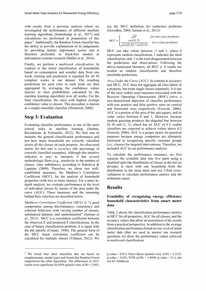
To answer RQ1, we consider the MCC and AUC values as described above. Considering the single-week classification results of all 50 weeks, we calculate the average performance and use a Student’s t-test to verify whether the AUC values are greater than 0.5 and the MCC values are greater than 0.
Based on these results, we can confirm the first research question (RQ1): It is indeed possible to predict eight of the eleven properties investigated (19 from 31 classes) with high confidence and better than a random guess. We achieved particularly good results for the prediction of properties related to the space and water heating system (space heating type, water heating type, and heat pump), the existence of photovoltaic or solar heat modules, as well as high and low number of appliances. We can also conclude that most of the properties that can be recognized well are energy-intensive (i.e., account for a large share of household electricity demand).
The accuracy and MCC results for multiweek classification, as also included in Table 2, are much higher than are results based on one week. Although the results based on all weeks might be over-fitted to the data, the figures show that there is room for algorithm improvement, which, however, is not the
focus of this paper. We present an analysis on the necessary number of weeks to exploit the performance gain from multiweek classification later in this paper. Interestingly, the classification performance of two properties that are similar to the study of Beckel et al. (2013, 2014) is higher or equal in our analysis: cooking type 89%/93% vs. 69%/71% and number of appliances 53%/60% vs. 53%/56% in single-week/multiweek classification. Beckel et al. predict also ‘age of house’ and achieve an accuracy of 60%/64% respectively, but define this property as a two-class problem (houses older than 30 years and newer ones) that usually leads to higher prediction accuracy results. The higher classification performance in this study might be due to our improved data processing (i.e., additional features, Random Forest classifier) or a result of the different datasets used.
Impact of temporal data resolution on classification performance
To investigate the first influencing factor, the classification procedure was applied for different data granularities with the following modification: We simulate different levels of data granularity by
Table 2: Classification performance for all properties and classes measured in MCC, AUC and accuracy on average based on all 50 weeks individually, and performance of multi-week classification
Single weeks (n=50) Multi-week classification Property Class AUC AUC > 0.51 MCC MCC>0.0a Accuracy MCC Accuracy 1 Space heating type Electric storage 0.6332 *** 0.3321 *** 80.82% 0.4693 87.59% Heat pump 0.6681 *** Other 0.6830 *** 2 Water heating type Electric storage 0.7890 *** 0.3940 *** 70.95% 0.5190 79.77% Heat pump 0.6558 *** Other 0.7610 *** 3 Age of heating Old 0.5370 0.1115 *** 40.50% 0.1666 44.71% Medium 0.6123 *** New 0.5612 * 4 Age of residency <10 0.5525 . 0.0980 *** 40.07% 0.1348 46.06% 10-29 0.5856 ** 30-74 0.5593 * >=75 0.4929 5 Heat pump No 0.6770 *** 0.2940 *** 82.53% 0.4900 89.66% Yes 0.6770 *** 6 Solar installation No 0.6312 *** 0.2854 *** 91.65% 0.3500 95.40% Yes 0.6312 *** 7 Num. of appliances Few 0.6984 *** 0.1519 *** 53.16% 0.2668 59.08% Moderate 0.5396 . Many 0.6144 *** 8 Interest in solar High 0.5984 *** 0.0777 *** 66.16% 0.0926 73.10% Moderate 0.5076 *** Low 0.6112 *** 9 Age of appliances New 0.4919 -0.0184 31.86% 0.0276 36.34% Moderate 0.4604 Old 0.4784 10 Cooking type Electric 0.4603 0.0596 * 89.10% 0.0700 92.87% Not electric 0.4603 11 Efficiency measures Multiple 0.4521 -0.0239 51.22% -0.0420 55.86% No 0.4980 One 0.4814 a) Significance code: '.' for p-value < 0.1, '*' for < 0.05, '**' for < 0.01, '***' for < 0.001
Smart Meter Data Analytics for Residential Energy Efficiency page 9/19
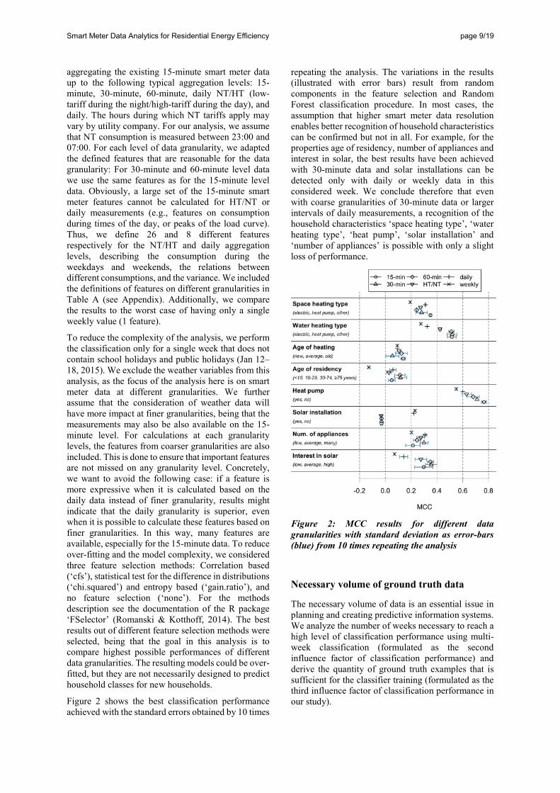
aggregating the existing 15-minute smart meter data up to the following typical aggregation levels: 15-minute, 30-minute, 60-minute, daily NT/HT (low-tariff during the night/high-tariff during the day), and daily. The hours during which NT tariffs apply may vary by utility company. For our analysis, we assume that NT consumption is measured between 23:00 and 07:00. For each level of data granularity, we adapted the defined features that are reasonable for the data granularity: For 30-minute and 60-minute level data we use the same features as for the 15-minute level data. Obviously, a large set of the 15-minute smart meter features cannot be calculated for HT/NT or daily measurements (e.g., features on consumption during times of the day, or peaks of the load curve). Thus, we define 26 and 8 different features respectively for the NT/HT and daily aggregation levels, describing the consumption during the weekdays and weekends, the relations between different consumptions, and the variance. We included the definitions of features on different granularities in Table A (see Appendix). Additionally, we compare the results to the worst case of having only a single weekly value (1 feature).
To reduce the complexity of the analysis, we perform the classification only for a single week that does not contain school holidays and public holidays (Jan 12–18, 2015). We exclude the weather variables from this analysis, as the focus of the analysis here is on smart meter data at different granularities. We further assume that the consideration of weather data will have more impact at finer granularities, being that the measurements may also be also available on the 15-minute level. For calculations at each granularity levels, the features from coarser granularities are also included. This is done to ensure that important features are not missed on any granularity level. Concretely, we want to avoid the following case: if a feature is more expressive when it is calculated based on the daily data instead of finer granularity, results might indicate that the daily granularity is superior, even when it is possible to calculate these features based on finer granularities. In this way, many features are available, especially for the 15-minute data. To reduce over-fitting and the model complexity, we considered three feature selection methods: Correlation based (‘cfs’), statistical test for the difference in distributions (‘chi.squared’) and entropy based (‘gain.ratio’), and no feature selection (‘none’). For the methods description see the documentation of the R package ‘FSelector’ (Romanski & Kotthoff, 2014). The best results out of different feature selection methods were selected, being that the goal in this analysis is to compare highest possible performances of different data granularities. The resulting models could be over-fitted, but they are not necessarily designed to predict household classes for new households.
Figure 2 shows the best classification performance achieved with the standard errors obtained by 10 times
repeating the analysis. The variations in the results (illustrated with error bars) result from random components in the feature selection and Random Forest classification procedure. In most cases, the assumption that higher smart meter data resolution enables better recognition of household characteristics can be confirmed but not in all. For example, for the properties age of residency, number of appliances and interest in solar, the best results have been achieved with 30-minute data and solar installations can be detected only with daily or weekly data in this considered week. We conclude therefore that even with coarse granularities of 30-minute data or larger intervals of daily measurements, a recognition of the household characteristics ‘space heating type’, ‘water heating type’, ‘heat pump’, ‘solar installation’ and ‘number of appliances’ is possible with only a slight loss of performance.
Figure 2: MCC results for different data granularities with standard deviation as error-bars (blue) from 10 times repeating the analysis
Necessary volume of ground truth data
The necessary volume of data is an essential issue in planning and creating predictive information systems. We analyze the number of weeks necessary to reach a high level of classification performance using multi-week classification (formulated as the second influence factor of classification performance) and derive the quantity of ground truth examples that is sufficient for the classifier training (formulated as the third influence factor of classification performance in our study).
Smart Meter Data Analytics for Residential Energy Efficiency page 10/19
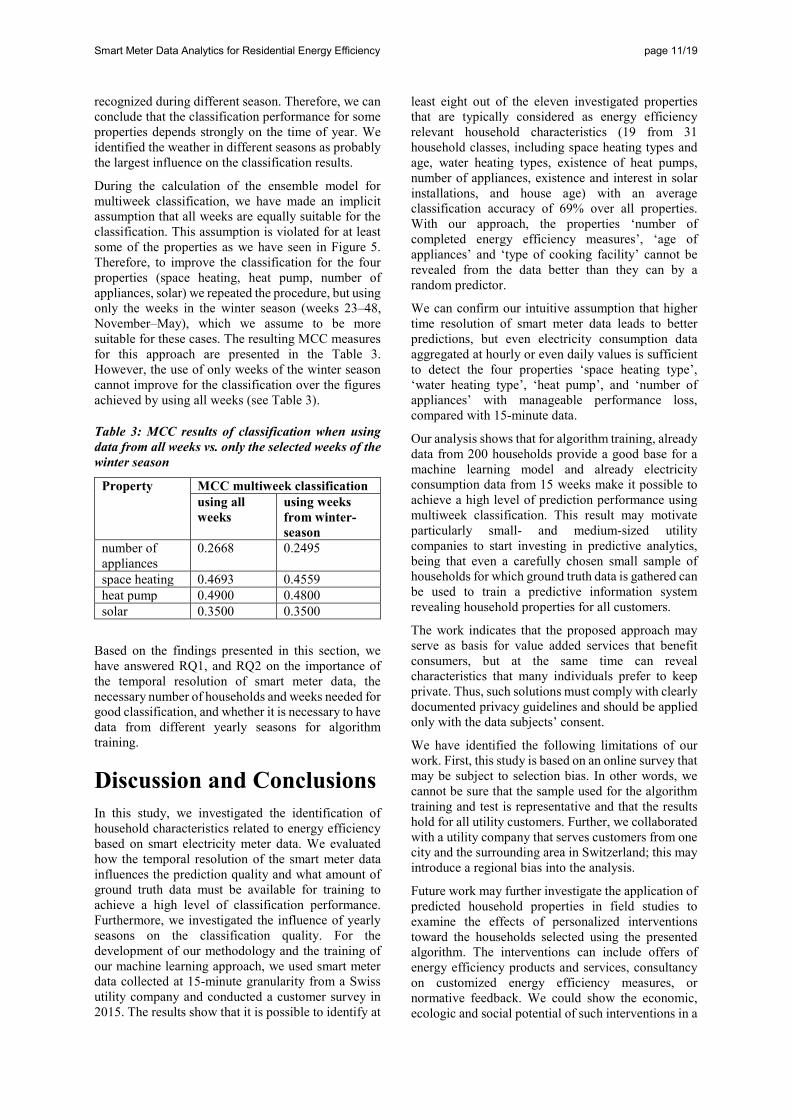
To find the number of weeks of smart meter data that is enough to improve classification with multi-week ensemble aggregation, we assess what time-span of data is required per household to reach a high level of classification performance. We perform the classification with an increasing number of weeks. The order of the weeks was randomized to avoid seasonal effects. All training examples are used in a 5-fold cross validation (i.e., for each iteration, 80% of the households are used for training and 20% of the data remain for the test) to calculate the result for the available dataset. Figure 3 shows the MCC for all eight recognizable properties with the increasing number of weeks.
We can conclude that a number of 15 weeks of smart meter data is enough to reach a high level of classification performance (see Figure 3). In detail, comparing the results achieved with classification based on 1–14 weeks with the results achieved with 16–50 weeks leads to 9.1% higher MCC results (paired t-test over all properties, t(295) = -6.8085, p-value < 0.0001).
Figure 3: MCC for all household properties then using different number of weeks
To test the necessary number of training instances to provide a high level of classification performance, we apply the classification setup and randomly separate the complete data into a training and a test set with the proportions 80% and 20%. We keep the size of the test set fixed and vary the size of the training set. For that, we randomly order the households in the training set and then select the first n household for the model training in 75 iterations. The resulting model in each iteration is then applied to the test set and the performance of predictions is calculated.
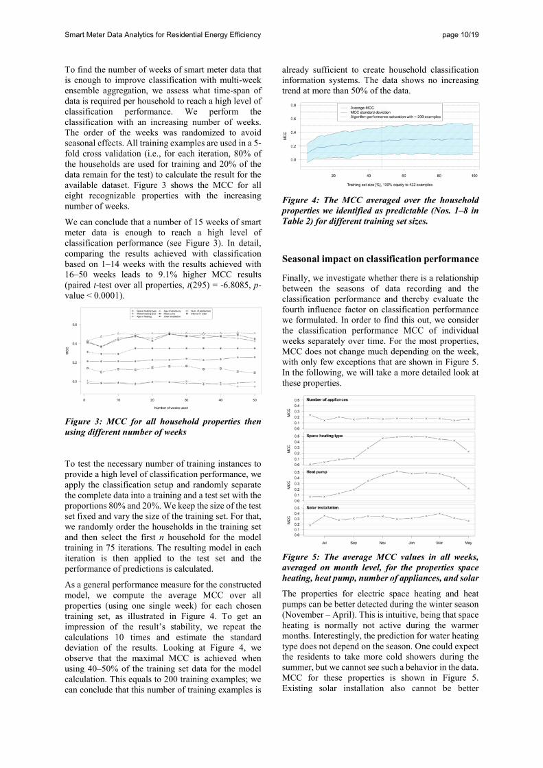
As a general performance measure for the constructed model, we compute the average MCC over all properties (using one single week) for each chosen training set, as illustrated in Figure 4. To get an impression of the result’s stability, we repeat the calculations 10 times and estimate the standard deviation of the results. Looking at Figure 4, we observe that the maximal MCC is achieved when using 40–50% of the training set data for the model calculation. This equals to 200 training examples; we can conclude that this number of training examples is
already sufficient to create household classification information systems. The data shows no increasing trend at more than 50% of the data.
Figure 4: The MCC averaged over the household properties we identified as predictable (Nos. 1–8 in Table 2) for different training set sizes.
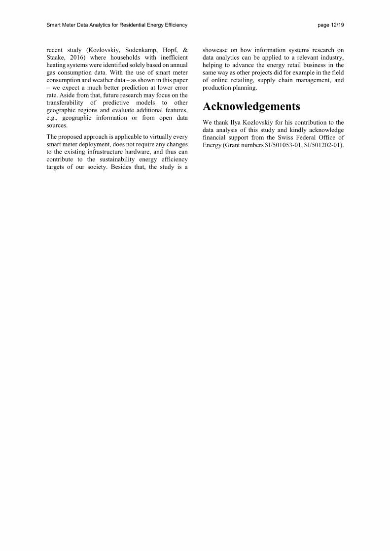
Seasonal impact on classification performance
Finally, we investigate whether there is a relationship between the seasons of data recording and the classification performance and thereby evaluate the fourth influence factor on classification performance we formulated. In order to find this out, we consider the classification performance MCC of individual weeks separately over time. For the most properties, MCC does not change much depending on the week, with only few exceptions that are shown in Figure 5. In the following, we will take a more detailed look at these properties.
Figure 5: The average MCC values in all weeks, averaged on month level, for the properties space heating, heat pump, number of appliances, and solar
The properties for electric space heating and heat pumps can be better detected during the winter season (November – April). This is intuitive, being that space heating is normally not active during the warmer months. Interestingly, the prediction for water heating type does not depend on the season. One could expect the residents to take more cold showers during the summer, but we cannot see such a behavior in the data. MCC for these properties is shown in Figure 5. Existing solar installation also cannot be better
Smart Meter Data Analytics for Residential Energy Efficiency page 11/19
recognized during different season. Therefore, we can conclude that the classification performance for some properties depends strongly on the time of year. We identified the weather in different seasons as probably the largest influence on the classification results.
During the calculation of the ensemble model for multiweek classification, we have made an implicit assumption that all weeks are equally suitable for the classification. This assumption is violated for at least some of the properties as we have seen in Figure 5. Therefore, to improve the classification for the four properties (space heating, heat pump, number of appliances, solar) we repeated the procedure, but using only the weeks in the winter season (weeks 23–48, November–May), which we assume to be more suitable for these cases. The resulting MCC measures for this approach are presented in the Table 3. However, the use of only weeks of the winter season cannot improve for the classification over the figures achieved by using all weeks (see Table 3).
Table 3: MCC results of classification when using data from all weeks vs. only the selected weeks of the winter season
Property MCC multiweek classification using all weeks
using weeks from winter-season
number of appliances
0.2668 0.2495
space heating 0.4693 0.4559 heat pump 0.4900 0.4800 solar 0.3500 0.3500
Based on the findings presented in this section, we have answered RQ1, and RQ2 on the importance of the temporal resolution of smart meter data, the necessary number of households and weeks needed for good classification, and whether it is necessary to have data from different yearly seasons for algorithm training.
Discussion and Conclusions In this study, we investigated the identification of household characteristics related to energy efficiency based on smart electricity meter data. We evaluated how the temporal resolution of the smart meter data influences the prediction quality and what amount of ground truth data must be available for training to achieve a high level of classification performance. Furthermore, we investigated the influence of yearly seasons on the classification quality. For the development of our methodology and the training of our machine learning approach, we used smart meter data collected at 15-minute granularity from a Swiss utility company and conducted a customer survey in 2015. The results show that it is possible to identify at
least eight out of the eleven investigated properties that are typically considered as energy efficiency relevant household characteristics (19 from 31 household classes, including space heating types and age, water heating types, existence of heat pumps, number of appliances, existence and interest in solar installations, and house age) with an average classification accuracy of 69% over all properties. With our approach, the properties ‘number of completed energy efficiency measures’, ‘age of appliances’ and ‘type of cooking facility’ cannot be revealed from the data better than they can by a random predictor.
We can confirm our intuitive assumption that higher time resolution of smart meter data leads to better predictions, but even electricity consumption data aggregated at hourly or even daily values is sufficient to detect the four properties ‘space heating type’, ‘water heating type’, ‘heat pump’, and ‘number of appliances’ with manageable performance loss, compared with 15-minute data.
Our analysis shows that for algorithm training, already data from 200 households provide a good base for a machine learning model and already electricity consumption data from 15 weeks make it possible to achieve a high level of prediction performance using multiweek classification. This result may motivate particularly small- and medium-sized utility companies to start investing in predictive analytics, being that even a carefully chosen small sample of households for which ground truth data is gathered can be used to train a predictive information system revealing household properties for all customers.
The work indicates that the proposed approach may serve as basis for value added services that benefit consumers, but at the same time can reveal characteristics that many individuals prefer to keep private. Thus, such solutions must comply with clearly documented privacy guidelines and should be applied only with the data subjects’ consent.
We have identified the following limitations of our work. First, this study is based on an online survey that may be subject to selection bias. In other words, we cannot be sure that the sample used for the algorithm training and test is representative and that the results hold for all utility customers. Further, we collaborated with a utility company that serves customers from one city and the surrounding area in Switzerland; this may introduce a regional bias into the analysis.
Future work may further investigate the application of predicted household properties in field studies to examine the effects of personalized interventions toward the households selected using the presented algorithm. The interventions can include offers of energy efficiency products and services, consultancy on customized energy efficiency measures, or normative feedback. We could show the economic, ecologic and social potential of such interventions in a
Smart Meter Data Analytics for Residential Energy Efficiency page 12/19
recent study (Kozlovskiy, Sodenkamp, Hopf, & Staake, 2016) where households with inefficient heating systems were identified solely based on annual gas consumption data. With the use of smart meter consumption and weather data – as shown in this paper – we expect a much better prediction at lower error rate. Aside from that, future research may focus on the transferability of predictive models to other geographic regions and evaluate additional features, e.g., geographic information or from open data sources.
The proposed approach is applicable to virtually every smart meter deployment, does not require any changes to the existing infrastructure hardware, and thus can contribute to the sustainability energy efficiency targets of our society. Besides that, the study is a
showcase on how information systems research on data analytics can be applied to a relevant industry, helping to advance the energy retail business in the same way as other projects did for example in the field of online retailing, supply chain management, and production planning.
Acknowledgements We thank Ilya Kozlovskiy for his contribution to the data analysis of this study and kindly acknowledge financial support from the Swiss Federal Office of Energy (Grant numbers SI/501053-01, SI/501202-01).
Smart Meter Data Analytics for Residential Energy Efficiency page 13/19
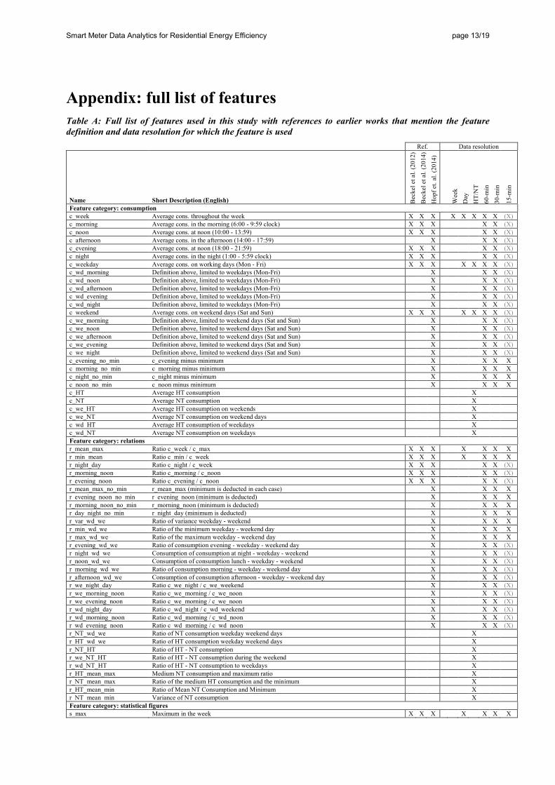
Appendix: full list of features Table A: Full list of features used in this study with references to earlier works that mention the feature definition and data resolution for which the feature is used
Ref. Data resolution
Name Short Description (English) Bec
kel e
t al.
(201
2)
Bec
kel e
t al.
(201
4)
Hop
f et.
al. (
2014
) W
eek
Day
H
T/N
T 60
-min
30
-min
15-m
in
Feature category: consumption c_week Average cons. throughout the week X X X X X X X X (X) c_morning Average cons. in the morning (6:00 - 9:59 clock) X X X X X (X) c_noon Average cons. at noon (10:00 - 13:59) X X X X X (X) c_afternoon Average cons. in the afternoon (14:00 - 17:59) X X X (X) c_evening Average cons. at noon (18:00 - 21:59) X X X X X (X) c_night Average cons. in the night (1:00 - 5:59 clock) X X X X X (X) c_weekday Average cons. on working days (Mon - Fri) X X X X X X X (X) c_wd_morning Definition above, limited to weekdays (Mon-Fri) X X X (X) c_wd_noon Definition above, limited to weekdays (Mon-Fri) X X X (X) c_wd_afternoon Definition above, limited to weekdays (Mon-Fri) X X X (X) c_wd_evening Definition above, limited to weekdays (Mon-Fri) X X X (X) c_wd_night Definition above, limited to weekdays (Mon-Fri) X X X (X) c_weekend Average cons. on weekend days (Sat and Sun) X X X X X X X (X) c_we_morning Definition above, limited to weekend days (Sat and Sun) X X X (X) c_we_noon Definition above, limited to weekend days (Sat and Sun) X X X (X) c_we_afternoon Definition above, limited to weekend days (Sat and Sun) X X X (X) c_we_evening Definition above, limited to weekend days (Sat and Sun) X X X (X) c_we_night Definition above, limited to weekend days (Sat and Sun) X X X (X) c_evening_no_min c_evening minus minimum X X X X c_morning_no_min c_morning minus minimum X X X X c_night_no_min c_night minus minimum X X X X c_noon_no_min c_noon minus minimum X X X X c_HT Average HT consumption X c_NT Average NT consumption X c_we_HT Average HT consumption on weekends X c_we_NT Average NT consumption on weekend days X c_wd_HT Average HT consumption of weekdays X c_wd_NT Average NT consumption on weekdays X Feature category: relations r_mean_max Ratio c_week / c_max X X X X X X X r_min_mean Ratio c_min / c_week X X X X X X X r_night_day Ratio c_night / c_week X X X X X (X) r_morning_noon Ratio c_morning / c_noon X X X X X (X) r_evening_noon Ratio c_evening / c_noon X X X X X (X) r_mean_max_no_min r_mean_max (minimum is deducted in each case) X X X X r_evening_noon_no_min r_evening_noon (minimum is deducted) X X X X r_morning_noon_no_min r_morning_noon (minimum is deducted) X X X X r_day_night_no_min r_night_day (minimum is deducted) X X X X r_var_wd_we Ratio of variance weekday - weekend X X X X r_min_wd_we Ratio of the minimum weekday - weekend day X X X X r_max_wd_we Ratio of the maximum weekday - weekend day X X X X r_evening_wd_we Ratio of consumption evening - weekday - weekend day X X X (X) r_night_wd_we Consumption of consumption at night - weekday - weekend X X X (X) r_noon_wd_we Consumption of consumption lunch - weekday - weekend X X X (X) r_morning_wd_we Ratio of consumption morning - weekday - weekend day X X X (X) r_afternoon_wd_we Consumption of consumption afternoon - weekday - weekend day X X X (X) r_we_night_day Ratio c_we_night / c_we_weekend X X X (X) r_we_morning_noon Ratio c_we_morning / c_we_noon X X X (X) r_we_evening_noon Ratio c_we_morning / c_we_noon X X X (X) r_wd_night_day Ratio c_wd_night / c_wd_weekend X X X (X) r_wd_morning_noon Ratio c_wd_morning / c_wd_noon X X X (X) r_wd_evening_noon Ratio c_wd_morning / c_wd_noon X X X (X) r_NT_wd_we Ratio of NT consumption weekday weekend days X r_HT_wd_we Ratio of HT consumption weekday weekend days X r_NT_HT Ratio of HT - NT consumption X r_we_NT_HT Ratio of HT - NT consumption during the weekend X r_wd_NT_HT Ratio of HT - NT consumption to weekdays X r_HT_mean_max Medium NT consumption and maximum ratio X r_NT_mean_max Ratio of the medium HT consumption and the minimum X r_HT_mean_min Ratio of Mean NT Consumption and Minimum X r_NT_mean_min Variance of NT consumption X Feature category: statistical figures s_max Maximum in the week X X X X X X X
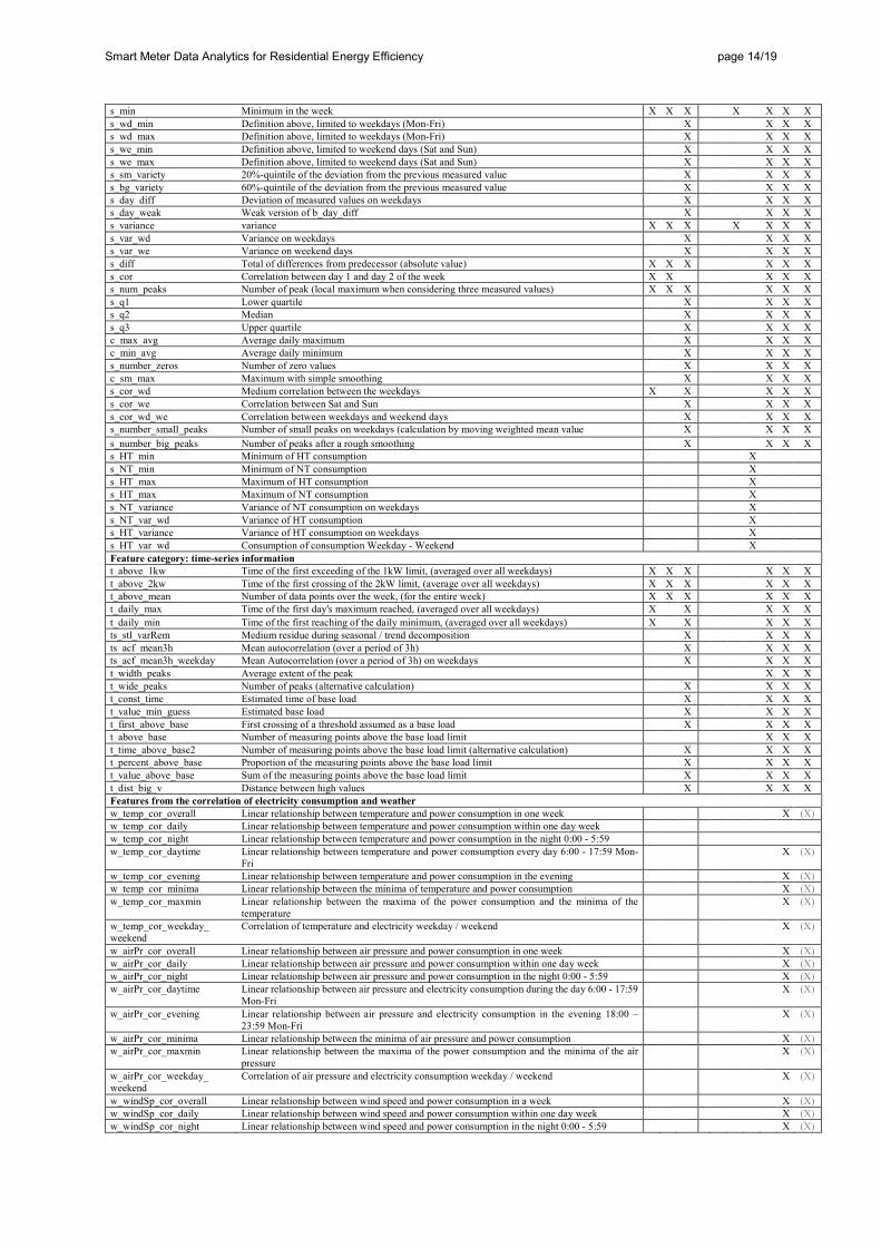
Smart Meter Data Analytics for Residential Energy Efficiency page 14/19
s_min Minimum in the week X X X X X X X s_wd_min Definition above, limited to weekdays (Mon-Fri) X X X X s_wd_max Definition above, limited to weekdays (Mon-Fri) X X X X s_we_min Definition above, limited to weekend days (Sat and Sun) X X X X s_we_max Definition above, limited to weekend days (Sat and Sun) X X X X s_sm_variety 20%-quintile of the deviation from the previous measured value X X X X s_bg_variety 60%-quintile of the deviation from the previous measured value X X X X s_day_diff Deviation of measured values on weekdays X X X X s_day_weak Weak version of b_day_diff X X X X s_variance variance X X X X X X X s_var_wd Variance on weekdays X X X X s_var_we Variance on weekend days X X X X s_diff Total of differences from predecessor (absolute value) X X X X X X s_cor Correlation between day 1 and day 2 of the week X X X X X s_num_peaks Number of peak (local maximum when considering three measured values) X X X X X X s_q1 Lower quartile X X X X s_q2 Median X X X X s_q3 Upper quartile X X X X c_max_avg Average daily maximum X X X X c_min_avg Average daily minimum X X X X s_number_zeros Number of zero values X X X X c_sm_max Maximum with simple smoothing X X X X s_cor_wd Medium correlation between the weekdays X X X X X s_cor_we Correlation between Sat and Sun X X X X s_cor_wd_we Correlation between weekdays and weekend days X X X X s_number_small_peaks Number of small peaks on weekdays (calculation by moving weighted mean value X X X X s_number_big_peaks Number of peaks after a rough smoothing X X X X s_HT_min Minimum of HT consumption X s_NT_min Minimum of NT consumption X s_HT_max Maximum of HT consumption X s_HT_max Maximum of NT consumption X s_NT_variance Variance of NT consumption on weekdays X s_NT_var_wd Variance of HT consumption X s_HT_variance Variance of HT consumption on weekdays X s_HT_var_wd Consumption of consumption Weekday - Weekend X Feature category: time-series information t_above_1kw Time of the first exceeding of the 1kW limit, (averaged over all weekdays) X X X X X X t_above_2kw Time of the first crossing of the 2kW limit, (average over all weekdays) X X X X X X t_above_mean Number of data points over the week, (for the entire week) X X X X X X t_daily_max Time of the first day's maximum reached, (averaged over all weekdays) X X X X X t_daily_min Time of the first reaching of the daily minimum, (averaged over all weekdays) X X X X X ts_stl_varRem Medium residue during seasonal / trend decomposition X X X X ts_acf_mean3h Mean autocorrelation (over a period of 3h) X X X X ts_acf_mean3h_weekday Mean Autocorrelation (over a period of 3h) on weekdays X X X X t_width_peaks Average extent of the peak X X X t_wide_peaks Number of peaks (alternative calculation) X X X X t_const_time Estimated time of base load X X X X t_value_min_guess Estimated base load X X X X t_first_above_base First crossing of a threshold assumed as a base load X X X X t_above_base Number of measuring points above the base load limit X X X t_time_above_base2 Number of measuring points above the base load limit (alternative calculation) X X X X t_percent_above_base Proportion of the measuring points above the base load limit X X X X t_value_above_base Sum of the measuring points above the base load limit X X X X t_dist_big_v Distance between high values X X X X Features from the correlation of electricity consumption and weather w_temp_cor_overall Linear relationship between temperature and power consumption in one week X (X) w_temp_cor_daily Linear relationship between temperature and power consumption within one day week w_temp_cor_night Linear relationship between temperature and power consumption in the night 0:00 - 5:59 w_temp_cor_daytime Linear relationship between temperature and power consumption every day 6:00 - 17:59 Mon-
Fri X (X)
w_temp_cor_evening Linear relationship between temperature and power consumption in the evening X (X) w_temp_cor_minima Linear relationship between the minima of temperature and power consumption X (X) w_temp_cor_maxmin Linear relationship between the maxima of the power consumption and the minima of the
temperature X (X)
w_temp_cor_weekday_ weekend
Correlation of temperature and electricity weekday / weekend X (X)
w_airPr_cor_overall Linear relationship between air pressure and power consumption in one week X (X) w_airPr_cor_daily Linear relationship between air pressure and power consumption within one day week X (X) w_airPr_cor_night Linear relationship between air pressure and power consumption in the night 0:00 - 5:59 X (X) w_airPr_cor_daytime Linear relationship between air pressure and electricity consumption during the day 6:00 - 17:59
Mon-Fri X (X)
w_airPr_cor_evening Linear relationship between air pressure and electricity consumption in the evening 18:00 – 23:59 Mon-Fri
X (X)
w_airPr_cor_minima Linear relationship between the minima of air pressure and power consumption X (X) w_airPr_cor_maxmin Linear relationship between the maxima of the power consumption and the minima of the air
pressure X (X)
w_airPr_cor_weekday_ weekend
Correlation of air pressure and electricity consumption weekday / weekend X (X)
w_windSp_cor_overall Linear relationship between wind speed and power consumption in a week X (X) w_windSp_cor_daily Linear relationship between wind speed and power consumption within one day week X (X) w_windSp_cor_night Linear relationship between wind speed and power consumption in the night 0:00 - 5:59 X (X)
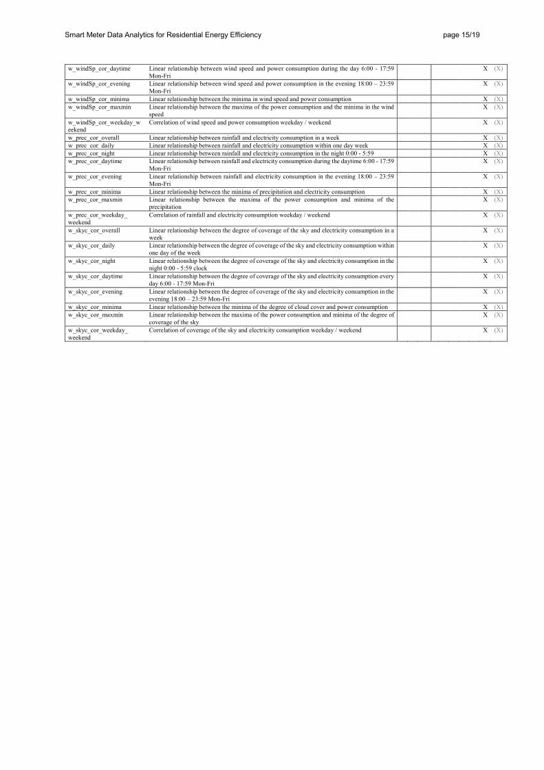
Smart Meter Data Analytics for Residential Energy Efficiency page 15/19
w_windSp_cor_daytime Linear relationship between wind speed and power consumption during the day 6:00 - 17:59 Mon-Fri
X (X)
w_windSp_cor_evening Linear relationship between wind speed and power consumption in the evening 18:00 – 23:59 Mon-Fri
X (X)
w_windSp_cor_minima Linear relationship between the minima in wind speed and power consumption X (X) w_windSp_cor_maxmin Linear relationship between the maxima of the power consumption and the minima in the wind
speed X (X)
w_windSp_cor_weekday_weekend
Correlation of wind speed and power consumption weekday / weekend X (X)
w_prec_cor_overall Linear relationship between rainfall and electricity consumption in a week X (X) w_prec_cor_daily Linear relationship between rainfall and electricity consumption within one day week X (X) w_prec_cor_night Linear relationship between rainfall and electricity consumption in the night 0:00 - 5:59 X (X) w_prec_cor_daytime Linear relationship between rainfall and electricity consumption during the daytime 6:00 - 17:59
Mon-Fri X (X)
w_prec_cor_evening Linear relationship between rainfall and electricity consumption in the evening 18:00 – 23:59 Mon-Fri
X (X)
w_prec_cor_minima Linear relationship between the minima of precipitation and electricity consumption X (X) w_prec_cor_maxmin Linear relationship between the maxima of the power consumption and minima of the
precipitation X (X)
w_prec_cor_weekday_ weekend
Correlation of rainfall and electricity consumption weekday / weekend X (X)
w_skyc_cor_overall Linear relationship between the degree of coverage of the sky and electricity consumption in a week
X (X)
w_skyc_cor_daily Linear relationship between the degree of coverage of the sky and electricity consumption within one day of the week
X (X)
w_skyc_cor_night Linear relationship between the degree of coverage of the sky and electricity consumption in the night 0:00 - 5:59 clock
X (X)
w_skyc_cor_daytime Linear relationship between the degree of coverage of the sky and electricity consumption every day 6:00 - 17:59 Mon-Fri
X (X)
w_skyc_cor_evening Linear relationship between the degree of coverage of the sky and electricity consumption in the evening 18:00 – 23:59 Mon-Fri
X (X)
w_skyc_cor_minima Linear relationship between the minima of the degree of cloud cover and power consumption X (X) w_skyc_cor_maxmin Linear relationship between the maxima of the power consumption and minima of the degree of
coverage of the sky X (X)
w_skyc_cor_weekday_ weekend
Correlation of coverage of the sky and electricity consumption weekday / weekend X (X)

Smart Meter Data Analytics for Residential Energy Efficiency page 16/19
References List Albert, A., & Rajagopal, R. (2013). Smart Meter Driven Segmentation: What Your Consumption Says About You. IEEE Transactions on Power Systems, 28(4), 4019–4030.
Albert, A., & Rajagopal, R. (2014). Cost-of-Service Segmentation of Energy Consumers. IEEE Transactions on Power Systems, 29(6), 2795–2803. https://doi.org/10.1109/TPWRS.2014.2312721
Allcott, H. (2011). Social norms and energy conservation. Journal of Public Economics, 95(9–10), 1082–1095. https://doi.org/10.1016/j.jpubeco.2011.03.003
Allcott, H., & Mullainathan, S. (2010). Behavior and energy policy. Science, 327(5970), 1204–1205.
Al-Otaibi, R., Jin, N., Wilcox, T., & Flach, P. (2016). Feature Construction and Calibration for Clustering Daily Load Curves from Smart-Meter Data. IEEE Transactions on Industrial Informatics, 12(2), 645–654. https://doi.org/10.1109/TII.2016.2528819
Armel, K. C., Gupta, A., Shrimali, G., & Albert, A. (2013). Is disaggregation the holy grail of energy efficiency? The case of electricity. Energy Policy, 52(Supplement C), 213–234. https://doi.org/10.1016/j.enpol.2012.08.062
Beckel, C., Sadamori, L., & Santini, S. (2012). Towards automatic classification of private households using electricity consumption data. In G. J. Pappas (Ed.), Proceedings of the Fourth ACM Workshop on Embedded Sensing Systems for Energy-Efficiency in Buildings (pp. 169–176). Toronto: ACM.
Beckel, C., Sadamori, L., & Santini, S. (2013). Automatic socio-economic classification of households using electricity consumption data. In D. Culler & C. Rosenberg (Eds.), Proceedings of the Fourth International Conference on Future Energy Systems (pp. 75–86). Berkeley, CA: ACM.
Beckel, C., Sadamori, L., Staake, T., & Santini, S. (2014). Revealing household characteristics from smart meter data. Energy, 78, 397–410.
Birt, B. J., Newsham, G. R., Beausoleil-Morrison, I., Armstrong, M. M., Saldanha, N., & Rowlands, I. H. (2012). Disaggregating categories of electrical energy end-use from whole-house hourly data. Energy and Buildings, 50, 93–102.
Breiman, L. (2001). Random forests. Machine Learning, 45(1), 5–32.
Buchanan, K., Banks, N., Preston, I., & Russo, R. (2016). The British public’s perception of the UK smart metering initiative: Threats and opportunities. Energy Policy, 91, 87–97. https://doi.org/10.1016/j.enpol.2016.01.003
Chang, H. H., Wong, K. H., & Fang, P. W. (2014). The effects of customer relationship management relational information processes on customer-based performance. Decision Support Systems, 66(Supplement C), 146–159. https://doi.org/10.1016/j.dss.2014.06.010
Chapman, P., Clinton, J., Kerber, R., Khabaza, T., Reinartz, T., Shearer, C., & Wirth, R. (2000). CRISP-DM 1.0. SPSS. Retrieved from ftp://ftp.software.ibm.com/software/analytics/spss/support/Modeler/Documentation/ 14/UserManual/CRISP-DM.pdf
Chicco, G. (2012). Overview and performance assessment of the clustering methods for electrical load pattern grouping. Energy, 42(1), 68–80.
Coltman, T. (2007). Why build a customer relationship management capability? The Journal of Strategic Information Systems, 16(3), 301–320. https://doi.org/10.1016/j.jsis.2007.05.001
Constantiou, I. D., & Kallinikos, J. (2015). New games, new rules: big data and the changing context of strategy. Journal of Information Technology, 30(1), 44–57. https://doi.org/10.1057/jit.2014.17
Cramer, H. (1946). Mathematical Methods of Statistics. Princeton, NJ: Princeton University Press.
Darby, S. (2006). The effectiveness of feedback on energy consumption. University of Oxford. Retrieved from http://www.usclcorp.com/news/DEFRA-report-with-appendix.pdf
de Silva, D., Xinghuo, Y., Alahakoon, D., & Holmes, G. (2011). A Data Mining Framework for Electricity Consumption Analysis From Meter Data. IEEE Transactions on Industrial Informatics, 7(3), 399–407.
Dietterich, T. G. (2000). Ensemble methods in machine learning. In International workshop on multiple classifier systems (pp. 1–15). Springer.
Ecoplan. (2015). Smart Metering Roll Out – Kosten und Nutzen: Aktualisierung des Smart Metering Impact Assessments 2012 (Final Report). Bern: Bundesamt für Energie. Retrieved from

Smart Meter Data Analytics for Residential Energy Efficiency page 17/19
http://www.bfe.admin.ch/php/modules/publikationen/stream.php?extlang=de&name=de_678554277.pdf&endung=Smart%20Metering%20Roll%20Out%20%96%20Kosten%20und%20Nutzen
European Commission. (2012, March 9). Commission Recommendation of 9 March 2012 on preparations for the roll-out of smart metering systems. Official Journal of the European Union. Retrieved from http://eur-lex.europa.eu/legal-content/EN/ALL/?uri=CELEX:32012H0148
European Commission. (2014). COMMISSION STAFF WORKING DOCUMENT Cost–benefit analyses & state of play of smart metering deployment in the EU-27 Accompanying the document Report from the Commission Benchmarking smart metering deployment in the EU-27 with a focus on electricity (COMMISSION STAFF WORKING DOCUMENT No. SWD/2014/0189). Brussels: European Commission.
Fawcett, T. (2006). An introduction to ROC analysis. Pattern Recognition Letters, 27(8), 861–874.
Fei, H., Kim, Y., Sahu, S., Naphade, M., Mamidipalli, S. K., & Hutchinson, J. (2013). Heat Pump Detection from Coarse Grained Smart Meter Data with Positive and Unlabeled Learning. In Proceedings of the 19th ACM SIGKDD International Conference on Knowledge Discovery and Data Mining (pp. 1330–1338). New York: ACM. https://doi.org/10.1145/2487575.2488203
Fernández-Delgado, M., Cernadas, E., Barro, S., & Amorim, D. (2014). Do we need hundreds of classifiers to solve real world classification problems? The Journal of Machine Learning Research, 15(1), 3133–3181.
Flath, C., Nicolay, D., Conte, T., Dinther, C. van, & Filipova-Neumann, L. (2012). Cluster Analysis of Smart Metering Data. Business & Information Systems Engineering, 4(1), 31–39. https://doi.org/10.1007/s12599-011-0201-5
Gorodkin, J. (2004). Comparing two K-category assignments by a K-category correlation coefficient. Computational Biology and Chemistry, 28(5), 367–374.
Graml, T., Loock, C.-M., Baeriswyl, M., & Staake, T. (2011). Improving Residential Energy Consumption at Large Using Persuasive Systems. In ECIS 2011 Proceedings. Helsinki, Finland: AIS electronic library.
Hart, G. W. (1992). Nonintrusive appliance load monitoring. Proceedings of the IEEE, 80(12), 1870–1891. https://doi.org/10.1109/5.192069
Hopf, K., Riechel, S., Sodenkamp, M., & Staake, T. (2017). Predictive Customer Data Analytics – The Value of Public Statistical Data and the Geographic Model Transferability. In ICIS 2017 Proceedings. Seoul, South Korea: AIS electronic library.
Hopf, K., Sodenkamp, M., & Kozlovskiy, I. (2016). Energy data analytics for improved residential service quality and energy efficiency. In ECIS 2016 Proceedings. Istanbul, Turkey: AIS electronic library.
Hopf, K., Sodenkamp, M., Kozlovskiy, I., & Staake, T. (2014). Feature extraction and filtering for household classification based on smart electricity meter data. In Computer Science-Research and Development (Vol. (31) 3, pp. 141–148). Zürich: Springer Berlin Heidelberg. https://doi.org/10.1007/s00450-014-0294-4
Jurman, G., Riccadonna, S., & Furlanello, C. (2012). A Comparison of MCC and CEN Error Measures in Multi-Class Prediction. PLoS ONE, 7(8). https://doi.org/10.1371/journal.pone.0041882
Keogh, E., & Mueen, A. (2011). Curse of Dimensionality. In C. Sammut & G. I. Webb (Eds.), Encyclopedia of Machine Learning (pp. 257–258). Springer US. https://doi.org/10.1007/978-0-387-30164-8_192
Kim, H., Marwah, M., Arlitt, M., Lyon, G., & Han, J. (2011). Unsupervised Disaggregation of Low Frequency Power Measurements. In Proceedings of the 2011 SIAM International Conference on Data Mining (Vols. 1–0, pp. 747–758). Society for Industrial and Applied Mathematics.
Kozlovskiy, I., Sodenkamp, M., Hopf, K., & Staake, T. (2016). Energy informatics for environmental, economic and social sustainability: A case of the large-scale detection of households with old heating systems. In ECIS 2016 Proceedings. Istanbul, Turkey: AIS electronic library.
Kwac, J., Tan, C.-W., Sintov, N., Flora, J., & Rajagopal, R. (2013). Utility customer segmentation based on smart meter data: Empirical study. In Smart Grid Communications (SmartGridComm), 2013 IEEE International Conference on (pp. 720–725). IEEE.
Lewington, J., De Chernatony, L., & Brown, A. (1996). Harnessing the Power of Database Marketing. Journal of Marketing Management, 12(4), 329–346.
Li, X., Bowers, C. P., & Schnier, T. (2010). Classification of Energy Consumption in Buildings With Outlier Detection. IEEE Transactions on Industrial Electronics, 57(11), 3639–3644.

Smart Meter Data Analytics for Residential Energy Efficiency page 18/19
https://doi.org/10.1109/TIE.2009.2027926
Liaw, A., & Wiener., M. (2015). randomForest: Breiman and Cutler’s Random Forests for Classification and Regression (Version 4.6-12). Retrieved from https://cran.r-project.org/web/packages/randomForest/index.html
Loock, C.-M., Staake, T., & Thiesse, F. (2013). Motivating energy-efficient behavior with green IS: an investigation of goal setting and the role of defaults. MIS Quarterly, 37(4), 1313–1332.
McKenna, E., Richardson, I., & Thomson, M. (2012). Smart meter data: Balancing consumer privacy concerns with legitimate applications. Energy Policy, 41, 807–814.
McKerracher, C., & Torriti, J. (2013). Energy consumption feedback in perspective: integrating Australian data to meta-analyses on in-home displays. Energy Efficiency, 6(2), 387–405. https://doi.org/10.1007/s12053-012-9169-3
McLoughlin, F., Duffy, A., & Conlon, M. (2012). Characterising domestic electricity consumption patterns by dwelling and occupant socio-economic variables: An Irish case study. Energy and Buildings, 48, 240–248.
Müller, O., Junglas, I., Brocke, J. vom, & Debortoli, S. (2016). Utilizing big data analytics for information systems research: challenges, promises and guidelines. European Journal of Information Systems, 25(4), 289–302. https://doi.org/10.1057/ejis.2016.2
Otim, S., & Grover, V. (2006). An empirical study on Web-based services and customer loyalty. European Journal of Information Systems, 15(6), 527–541. https://doi.org/10.1057/palgrave.ejis.3000652
Romanski, P., & Kotthoff, L. (2014). FSelector: Selecting attributes. Retrieved from http://CRAN.R-project.org/package=FSelector
Sodenkamp, M., Kozlovskiy, I., Hopf, K., & Staake, T. (2017). Smart Meter Data Analytics for Enhanced Energy Efficiency in the Residential Sector. In Wirtschaftsinformatik 2017 Proceedings. St. Gallen, Switzerland: AIS electronic library.
Sokolova, M., & Lapalme, G. (2009). A systematic analysis of performance measures for classification tasks. Information Processing & Management, 45(4), 427–437.
Swiss Federal Statistical Office. (2017). Sustainable development, regional and international disparities / Statistical basis and overviews (Dataset No. FSO: je-d-21.03.01). Retrieved from https://www.bfs.admin.ch/bfs/en/home/statistics/regional-statistics/regional-portraits-key-figures/communes.assetdetail.2422865.html
Synnott, W. R. (1978). Total Customer Relationship. MIS Quarterly, 2(3), 15–24.
Tiefenbeck, V. (2017). Bring behaviour into the digital transformation. Nature Energy, 2(6), 17085. https://doi.org/10.1038/nenergy.2017.85
Tiefenbeck, V., Goette, L., Degen, K., Tasic, V., Fleisch, E., Lalive, R., & Staake, T. (2016). Overcoming Salience Bias: How Real-Time Feedback Fosters Resource Conservation. Management Science. https://doi.org/10.1287/mnsc.2016.2646
U.S. Energy Information Administration. (2017, December 8). How many smart meters are installed in the United States, and who has them? Retrieved January 18, 2018, from https://www.eia.gov/tools/faqs/faq.php?id=108&t=3
U.S. National Centers for Environmental Information. (2016). Climate Data Online. Retrieved January 2, 2016, from http://www.ncdc.noaa.gov/cdo-web/
Verma, A., Asadi, A., Yang, K., & Tyagi, S. (2015). A data-driven approach to identify households with plug-in electrical vehicles (PEVs). Applied Energy, 160(Supplement C), 71–79. https://doi.org/10.1016/j.apenergy.2015.09.013
Vihinen, M. (2012). How to evaluate performance of prediction methods? Measures and their interpretation in variation effect analysis. BMC Genomics, 13(4), S2. https://doi.org/10.1186/1471-2164-13-S4-S2
Watson, R. T., Boudreau, M.-C., & Chen, A. J. (2010). Information systems and environmentally sustainable development: energy informatics and new directions for the IS community.(Essay). MIS Quarterly, 34(1), 23.
Watson, R. T., Howells, J., & Boudreau, M.-C. (2012). Energy Informatics: Initial Thoughts on Data and Process Management. In J. vom Brocke, S. Seidel, & J. Recker (Eds.), Green Business Process Management (pp. 147–159). Springer Berlin Heidelberg. https://doi.org/10.1007/978-3-642-27488-6_9
Wattal, S., Telang, R., Mukhopadhyay, T., & Boatwright, P. (2011). What’s in a “Name”? Impact of Use of

Smart Meter Data Analytics for Residential Energy Efficiency page 19/19
Customer Information in E-Mail Advertisements. Information Systems Research, 23(3-part-1), 679–697. https://doi.org/10.1287/isre.1110.0384
Xu, M., & Walton, J. (2005). Gaining customer knowledge through analytical CRM. Industrial Management & Data Systems, 105(7), 955–971. https://doi.org/10.1108/02635570510616139
Yoo, Y. (2015). It is not about size: a further thought on big data. Journal of Information Technology, 30(1), 63–65. https://doi.org/10.1057/jit.2014.30
Zhang, T. C., Agarwal, R., & Lucas, J., Henry C. (2011). The Value of It-Enabled Retailer Learning: Personalized Product Recommendations and Customer Store Loyalty in Electronic Markets. MIS Quarterly, 35(4), 859-A7.


