Enhancements to the Generalized Sidelobe Canceller for ...

University of Kentucky University of Kentucky

UKnowledge UKnowledge

University of Kentucky Master's Theses Graduate School

2009

Enhancements to the Generalized Sidelobe Canceller for Audio Enhancements to the Generalized Sidelobe Canceller for Audio

Beamforming in an Immersive Environment Beamforming in an Immersive Environment

Phil Townsend University of Kentucky, [email protected]

Right click to open a feedback form in a new tab to let us know how this document benefits you. Right click to open a feedback form in a new tab to let us know how this document benefits you.

Recommended Citation Recommended Citation Townsend, Phil, "Enhancements to the Generalized Sidelobe Canceller for Audio Beamforming in an Immersive Environment" (2009). University of Kentucky Master's Theses. 645. https://uknowledge.uky.edu/gradschool_theses/645

This Thesis is brought to you for free and open access by the Graduate School at UKnowledge. It has been accepted for inclusion in University of Kentucky Master's Theses by an authorized administrator of UKnowledge. For more information, please contact [email protected].

http://uknowledge.uky.edu/

http://uknowledge.uky.edu/

https://uknowledge.uky.edu/

https://uknowledge.uky.edu/gradschool_theses

https://uknowledge.uky.edu/gradschool

https://uky.az1.qualtrics.com/jfe/form/SV_9mq8fx2GnONRfz7

mailto:[email protected]

ABSTRACT OF THESIS

Enhancements to the Generalized Sidelobe Canceller for Audio Beamforming in anImmersive Environment

The Generalized Sidelobe Canceller is an adaptive algorithm for optimally estimatingthe parameters for beamforming, the signal processing technique of combining datafrom an array of sensors to improve SNR at a point in space. This work focuseson the algorithm’s application to widely-separated microphone arrays with irregulardistributions used for human voice capture. Methods are presented for improvingthe performance of the algorithm’s blocking matrix, a stage that creates a noisereference for elimination, by proposing a stochastic model for amplitude correctionand enhanced use of cross correlation for phase correction and time-difference ofarrival estimation via a correlation coefficient threshold. This correlation techniqueis also applied to a multilateration algorithm for an efficient method of explicit targettracking. In addition, the underlying microphone array geometry is studied withparameters and guidelines for evaluation proposed. Finally, an analysis of the stabilityof the system is performed with respect to its adaptation parameters.

Multimedia Elements Used: WAV (.wav)

KEYWORDS: Beamforming, Digital Signal Processing, Microphone Arrays, AudioSignal Processing, Stochastics

Author’s signature: Phil Townsend

Date: December 15, 2009


ByPhil Townsend

Director of Thesis: Kevin D. Donohue

Director of Graduate Studies: Stephen Gedney

Date: December 15, 2009

RULES FOR THE USE OF THESES

Unpublished theses submitted for the Masters degree and deposited in the Universityof Kentucky Library are as a rule open for inspection, but are to be used only withdue regard to the rights of the authors. Bibliographical references may be noted, butquotations or summaries of parts may be published only with the permission of theauthor, and with the usual scholarly acknowledgments.

Extensive copying or publication of the thesis in whole or in part also requires theconsent of the Dean of the graduate School of the University of Kentucky.

A library that borrows this thesis for use by its patrons is expected to secure thesignature of each user.

Name Date

THESIS

Phil Townsend

The Graduate SchoolUniversity of Kentucky

2009


THESIS

A thesis submitted in partialfulfillment of the requirements forthe degree of Master of Science in

Electrical Engineering in the Collegeof Engineering at the University of

Kentucky

ByPhil Townsend

Lexington, Kentucky

Director: Dr. Kevin D. Donohue, Professor of Electrical and Computer EngineeringLexington, Kentucky 2009

Copyright c© Phil Townsend 2009

To my loving parents Ralf and Catherine, as well as my close friends Em, Katie,Robert, and Richard.

ACKNOWLEDGMENTS

First and foremost I’m deeply thankful to my advisor, Dr. Kevin Donohue, for his

support during my work at the University of Kentucky. His patient guidance as both

professor and mentor through the thesis process and during the several classes he’s

taught me throughout my academic career has been exceptional.

I’d like to thank everyone at the UK Vis Center for their support and discussion

of our audio work and in particular Drs. Jens Hannemann and Samson Cheung for

agreeing to take the time to sit for my defense committee.

And finally, I’d like to thank all my of my family members and closest friends for

their love and support during my college career as it’s led me to the completion of

this thesis and beyond.

iii

TABLE OF CONTENTS

Acknowledgments . . . . . . . . . . . . . . . . . . . . . . . . . . . . . . . . . iii

List of Figures . . . . . . . . . . . . . . . . . . . . . . . . . . . . . . . . . . . vii

List of Tables . . . . . . . . . . . . . . . . . . . . . . . . . . . . . . . . . . . . ix

List of Files . . . . . . . . . . . . . . . . . . . . . . . . . . . . . . . . . . . . x

Chapter 1 Introduction and Literature Review . . . . . . . . . . . . . . . . 11.1 A Brief History and Motivation for Study . . . . . . . . . . . . . . . . 11.2 The Basics of Beamforming . . . . . . . . . . . . . . . . . . . . . . . 2

1.2.1 A Continuous Aperture . . . . . . . . . . . . . . . . . . . . . . 21.2.2 The Delay-Sum Beamformer . . . . . . . . . . . . . . . . . . . 2

1.3 Adaptive Beamforming . . . . . . . . . . . . . . . . . . . . . . . . . . 31.3.1 Frost’s Algorithm . . . . . . . . . . . . . . . . . . . . . . . . . 31.3.2 The Generalized Sibelobe Canceller (Griffiths-Jim Beamformer) 7

1.4 Limitations of Current Models and Methods . . . . . . . . . . . . . . 81.5 Intelligibility and the SII Model . . . . . . . . . . . . . . . . . . . . . 91.6 The Audio Data Archive . . . . . . . . . . . . . . . . . . . . . . . . . 101.7 Organization of Thesis . . . . . . . . . . . . . . . . . . . . . . . . . . 10

Chapter 2 Statistical Amplitude Correction . . . . . . . . . . . . . . . . . . 122.1 Introduction . . . . . . . . . . . . . . . . . . . . . . . . . . . . . . . . 122.2 Manipulating Track Order . . . . . . . . . . . . . . . . . . . . . . . . 122.3 Models . . . . . . . . . . . . . . . . . . . . . . . . . . . . . . . . . . . 13

2.3.1 Spherical Wave Propagation in a Lossless Medium . . . . . . . 132.3.2 Air as a Lossy Medium and the ISO Model . . . . . . . . . . . 142.3.3 Statistical Blocking Matrix Energy Minimization . . . . . . . 16

2.4 Simulating a Perfect Blocking Matrix . . . . . . . . . . . . . . . . . . 192.5 Experimental Evaluation . . . . . . . . . . . . . . . . . . . . . . . . . 202.6 Results and Discussion . . . . . . . . . . . . . . . . . . . . . . . . . . 22

2.6.1 Example WAV’s Included with ETD . . . . . . . . . . . . . . 252.7 Conclusion . . . . . . . . . . . . . . . . . . . . . . . . . . . . . . . . . 25

Chapter 3 Automatic Steering Using Cross Correlation . . . . . . . . . . . . 273.1 Introduction . . . . . . . . . . . . . . . . . . . . . . . . . . . . . . . . 273.2 The GCC and PHAT Weighting Function . . . . . . . . . . . . . . . 273.3 Proposed Improvements . . . . . . . . . . . . . . . . . . . . . . . . . 28

3.3.1 Windowing of Data . . . . . . . . . . . . . . . . . . . . . . . . 293.3.2 Partial Whitening . . . . . . . . . . . . . . . . . . . . . . . . . 293.3.3 Windowed Cross Correlation . . . . . . . . . . . . . . . . . . . 29

iv

3.3.4 Correlation Coefficient Threshold . . . . . . . . . . . . . . . . 303.4 Multilateration . . . . . . . . . . . . . . . . . . . . . . . . . . . . . . 303.5 Experimental Evaluation . . . . . . . . . . . . . . . . . . . . . . . . . 32

3.5.1 GSC Performance with Automatic Steering . . . . . . . . . . . 323.5.2 Multilateration Versus SRP . . . . . . . . . . . . . . . . . . . 33

3.6 Results and Discussion . . . . . . . . . . . . . . . . . . . . . . . . . . 373.6.1 Example WAV’s Included with ETD . . . . . . . . . . . . . . 41

3.7 Conclusion . . . . . . . . . . . . . . . . . . . . . . . . . . . . . . . . . 41

Chapter 4 Microphone Geometry . . . . . . . . . . . . . . . . . . . . . . . . 434.1 Introduction . . . . . . . . . . . . . . . . . . . . . . . . . . . . . . . . 434.2 Limitations of an Equispaced Linear Array . . . . . . . . . . . . . . . 434.3 Generating and Visualizing 3D Beampatterns . . . . . . . . . . . . . 444.4 A Collection of Geometries . . . . . . . . . . . . . . . . . . . . . . . . 45

4.4.1 One Dimensional Arrays . . . . . . . . . . . . . . . . . . . . . 464.4.1.1 Linear Array . . . . . . . . . . . . . . . . . . . . . . 46

4.4.2 Two Dimensional Arrays . . . . . . . . . . . . . . . . . . . . . 474.4.2.1 Rectangular Array . . . . . . . . . . . . . . . . . . . 474.4.2.2 Perimeter Array . . . . . . . . . . . . . . . . . . . . 474.4.2.3 Random Ceiling Array 1 . . . . . . . . . . . . . . . . 504.4.2.4 Random Ceiling Array 2 . . . . . . . . . . . . . . . . 51

4.4.3 Three Dimensional Arrays . . . . . . . . . . . . . . . . . . . . 514.4.3.1 Corner Cluster . . . . . . . . . . . . . . . . . . . . . 514.4.3.2 Endfire Cluster . . . . . . . . . . . . . . . . . . . . . 544.4.3.3 Pairwise Even 3D Array . . . . . . . . . . . . . . . . 544.4.3.4 Spread Cluster Array . . . . . . . . . . . . . . . . . . 54

4.4.4 Comparison of Beamfields to Earlier Experimental Results . . 574.5 A Monte Carlo Experiment for Analysis of Geometry . . . . . . . . . 58

4.5.1 Proposed Parameters . . . . . . . . . . . . . . . . . . . . . . . 584.5.2 Experimental Setup . . . . . . . . . . . . . . . . . . . . . . . . 584.5.3 Results . . . . . . . . . . . . . . . . . . . . . . . . . . . . . . . 59

4.6 Guidelines for Optimal Microphone Placement . . . . . . . . . . . . . 614.7 Conclusions . . . . . . . . . . . . . . . . . . . . . . . . . . . . . . . . 62

Chapter 5 Final Conclusions and Future Work . . . . . . . . . . . . . . . . 63

Appendices . . . . . . . . . . . . . . . . . . . . . . . . . . . . . . . . . . . . . 65

Chapter A Stability Bounds for the GSC . . . . . . . . . . . . . . . . . . . . 65A.1 Introduction . . . . . . . . . . . . . . . . . . . . . . . . . . . . . . . . 65A.2 Derivation . . . . . . . . . . . . . . . . . . . . . . . . . . . . . . . . . 66A.3 Computer Verification . . . . . . . . . . . . . . . . . . . . . . . . . . 68A.4 Discussion . . . . . . . . . . . . . . . . . . . . . . . . . . . . . . . . . 70A.5 Conclusion . . . . . . . . . . . . . . . . . . . . . . . . . . . . . . . . . 71

v

Bibliography . . . . . . . . . . . . . . . . . . . . . . . . . . . . . . . . . . . . 72

Vita . . . . . . . . . . . . . . . . . . . . . . . . . . . . . . . . . . . . . . . . . 74

vi

LIST OF FIGURES

1.1 Frost’s Beamformer . . . . . . . . . . . . . . . . . . . . . . . . . . . . . . 41.2 The Generalized Sidelobe Canceller . . . . . . . . . . . . . . . . . . . . . 71.3 The SII Band Importance Spectrum . . . . . . . . . . . . . . . . . . . . 10

2.1 Example Griffiths-Jim Blocking Matrix for a Four-Channel Beamformer . 132.2 Blocking Matrix for Spherical Lossless Model . . . . . . . . . . . . . . . 152.3 Sound Propagation Model as a Cascade of Filters . . . . . . . . . . . . . 152.4 Blocking Matrix for ISO Sound Absorption Model in Frequency Domain 162.5 Statistical Blocking Matrix in Frequency Domain. . . . . . . . . . . . . . 182.6 GSC Ideal Target Cancellation Simulation Signal Flow Diagram. . . . . . 192.7 GSC Output Bar Chart for Data in Table 2.2 . . . . . . . . . . . . . . . 232.8 BM Bar Chart for Data in Table 2.3 . . . . . . . . . . . . . . . . . . . . 232.9 Sample Magnitude Spectrum for Statistical BM . . . . . . . . . . . . . . 242.10 Magnitude and Phase Response for ISO Filter, d = 3m . . . . . . . . . . 24

3.1 Bar Chart of GSC Output Track Correlations w/ Target . . . . . . . . . 343.2 Bar Chart of BM Output Track Correlations w/ Target . . . . . . . . . . 353.3 Bar Chart of Correlations from Table 3.3 . . . . . . . . . . . . . . . . . . 363.4 Bar Chart of Mean Errors vs SSL from Table 3.4 . . . . . . . . . . . . . 373.5 Multilateration and SSL Target Positions, ρthresh = .1 . . . . . . . . . . . 383.6 Multilateration and SSL Target Positions, ρthresh = .5 . . . . . . . . . . . 383.7 Multilateration and SSL Target Positions, ρthresh = .9 . . . . . . . . . . . 393.8 Multilateration and SSL Target Positions, ρthresh = .1 . . . . . . . . . . . 393.9 Multilateration and SSL Target Positions, ρthresh = .5 . . . . . . . . . . . 403.10 Multilateration and SSL Target Positions, ρthresh = .9 . . . . . . . . . . . 40

4.1 Linear Array Beamfield, Bird’s Eye View . . . . . . . . . . . . . . . . . . 464.2 Linear Array Beamfield, Perspective View . . . . . . . . . . . . . . . . . 474.3 Rectangular Array Beamfield, Bird’s Eye View . . . . . . . . . . . . . . . 484.4 Rectangular Array Beamfield, Perspective View . . . . . . . . . . . . . . 484.5 Perimeter Array Beamfield, Bird’s Eye View . . . . . . . . . . . . . . . . 494.6 Perimeter Array Beamfield, Perspective View . . . . . . . . . . . . . . . 494.7 First Random Array Beamfield, Bird’s Eye View . . . . . . . . . . . . . . 504.8 First Random Array Beamfield, Perspective View . . . . . . . . . . . . . 504.9 Second Random Array Beamfield, Bird’s Eye View . . . . . . . . . . . . 514.10 Second Random Array Beamfield, Perspective View . . . . . . . . . . . . 524.11 Corner Array Beamfield, Bird’s Eye View . . . . . . . . . . . . . . . . . 524.12 Corner Array Beamfield, Perspective View . . . . . . . . . . . . . . . . . 534.13 Endfire Cluster Beamfield, Bird’s Eye View . . . . . . . . . . . . . . . . 534.14 Endfire Cluster Beamfield, Perspective View . . . . . . . . . . . . . . . . 544.15 Pairwise Even 3D Beamfield, Bird’s Eye View . . . . . . . . . . . . . . . 55

vii

4.16 Pairwise Even 3D Beamfield, Perspective View . . . . . . . . . . . . . . . 554.17 Spread Cluster Beamfield, Bird’s Eye View . . . . . . . . . . . . . . . . . 564.18 Spread Cluster Beamfield, Perspective View . . . . . . . . . . . . . . . . 564.19 Error Bar Plot for Varying Array Centroid Displacement. . . . . . . . . 604.20 Error Bar Plot for Varying Array Dispersion. . . . . . . . . . . . . . . . 61

A.1 GSC Stability Plot, M = 2, βmax = .95, Voice Input . . . . . . . . . . . . 68A.2 GSC Stability Plot, M = 3, βmax = .95, Voice Input . . . . . . . . . . . . 69A.3 GSC Stability Plot, M = 4, βmax = .95, Voice Input . . . . . . . . . . . . 69A.4 GSC Stability Plot, M = 4, βmax = 1, Voice Input . . . . . . . . . . . . . 70A.5 GSC Stability Plot, M = 4, βmax = 1, Colored Noise Input . . . . . . . . 71

viii

LIST OF TABLES

2.1 Parameters for Amplitude Correction Tests . . . . . . . . . . . . . . . . . 212.2 GSC Mean Correlation Coefficients, BM Amplitude Correction . . . . . . 222.3 BM Track Mean Correlation Coefficient for Various Arrays and Models . 22

3.1 GSC Mean Correlation Coefficients, Automatic Steering . . . . . . . . . 333.2 BM Mean Correlation Coefficients, Automatic Steering . . . . . . . . . . 333.3 Beamformer Output Correlations for Various Thresholds . . . . . . . . . 353.4 Mean Multilateration Errors vs SSL for Various Thresholds . . . . . . . . 36

ix

LIST OF FILES

Clicking on the file name will play the selected WAV file in your environment’s defaultaudio player.

1. Amplitude Correction Sound Files (Chapter 2)

a) Linear Array

i. Target Speaker Alone: target.wav (1.1 MB)

ii. Cocktail Party Closest Mic: closestMic.wav (1.1 MB)

iii. Traditional GJBF Overall Output: yStandard.wav (1.1 MB)

iv. 1/r Model Overall Output: y1r.wav (1.1 MB)

v. ISO Model Overall Output: yIso.wav (1.1 MB)

vi. Statistical Model Overall Output: yStat.wav (1.1 MB)

vii. Perfect BM Overall Output: yPerfect.wav (1.1 MB)

b) Perimeter Array

i. Target Speaker Alone: target.wav (1.1 MB)

ii. Cocktail Party Closest Mic: closestMic.wav (1.1 MB)

iii. Traditional GJBF Overall Output: yStandard.wav (1.1 MB)

iv. 1/r Model Overall Output: y1r.wav (1.1 MB)

v. ISO Model Overall Output: yIso.wav (1.1 MB)

vi. Statistical Model Overall Output: yStat.wav (1.1 MB)

vii. Perfect BM Overall Output: yPerfect.wav (1.1 MB)

2. Cross Correlation Sound Files for Linear Array (Chapter 3)

a) ρthresh = .1: y1.wav (1.1 MB)

b) ρthresh = .5: y5.wav (1.1 MB)

c) ρthresh = .9: y9.wav (1.1 MB)

x

Chapter 1

Introduction and LiteratureReview

1.1 A Brief History and Motivation for Study

Beamforming is a spatial filtering technique that isolates sound sources based on theirpositions in space [1]. The technique originated in radio astronomy during the 1950’sas a way of combining antenna information from collections of antenna dishes, butby the 1970’s beamforming began to be explored as a generalized signal processingtechnique for any application involving spatially-distributed sensors. Examples of thisexpansion include sonar, to allow submarines greater ability to detect enemy shipsusing hydrophones, or in geology, enhancing the ability of ground sensors to detectand locate tectonic plate shifts [2].

It was around this time that microphone array beamforming in particular becamean active area of research, where the practice amounts to placing a virtual micro-phone at some position without physical sensor movement. Applications of audiobeamforming include hands-free listening and tracking of sound sources for notetak-ing in an office environment, issuing verbal commands to a computer, or surveillancewith a hidden array. In the present day the implementation cost of an array is lowenough to be a feasible technology for the consumer market. In fact, some commonPC software packages currently support small scale arrays such as Microsoft WindowsVista [3].

The present state of the art has seem some ability to improve acoustic SNR (signalto noise ratio) through the use of a microphone array but the performance still leavesmuch to be desired, especially under poor SNR conditions [2]. It is currently believedthat nonlinear techniques, such as the adaptive Generalized Sidelobe Canceller (GSC),will likely provide the most benefits given further study. Hence the study of the GSC,along with several attempts to improve its performance at enhancing human voicecapture, will be the focus of this work. In particular, we’ll study what’s referred toas the cocktail party problem, where we attempt to pull a human voice at one spatiallocation out of an acoustic scene that has several competing human voices at differentlocations.

1

1.2 The Basics of Beamforming

1.2.1 A Continuous Aperture

The concept of a beamformer is derived from the study of a theoretical continuousaperture (a spatial region that transmits or receives propagating waves) and modelinga microphone array as a sampled version at discrete points in space. The techniquecan be briefly formulated by first expressing the signal received by the aperture asthe application of a linear filter to some wave at all points along the aperture via theconvolution [4]

xR(t, r) =

∫ ∞

−∞

x(τ, r)a(t − τ, r)dτ (1.1)

where x(t, r) is the signal at time t and spatial location r and a(t, r) is the impulseresponse of the receiving aperture at t and r. Equivalently, the Fourier transform of(1.1) yields the frequency domain representation

XR(f, r) = X(f, r)A(f, r) (1.2)

where A(f, r) is called the aperture function, as it describes the sensitivity of thereceiving aperture as a function of frequency and position along the array. It canbe shown that the far field directivity pattern, or beampattern, which describes thereceived signal as a function of position in space for sources significantly distant fromthe array (Fresnel number F << 1), is the Fourier transform of the aperture function

D(f,α) = F{A(f, r)} =

∫ ∞

−∞

A(f, r)ej2πα·rdr (1.3)

where α is the three-element direction vector of a wave in spherical coordinates

α =1

λ[ sin θ cos φ sin θ sin φ cos θ ]

= [ αx αy αz ](1.4)

with θ the zenith angle, φ the azimuth angle, λ the sound source wavelength andthe elements of the vector corresponding to the x, y, and z Cartesian directions,respectively.

1.2.2 The Delay-Sum Beamformer

The Delay-Sum Beamformer (DSB) is the simplest of the beamforming algorithmsand follows closely from the above discussion of a continuous aperture. The DSBarises when one transforms the integration in (1.3) to a summation over a discretenumber of microphones and models the aperture function as a set of complex weightswn that may be chosen freely for each microphone.

D(f,α) =M∑

n=1

wn(f)ej2πα·rn (1.5)

2

where M is the number of microphones in the array. If one chooses wn as a set ofpurely phase terms the beamfield shape will be maintained 1 but its peak will shift,where if

wn(f) = e−j2πα′·rn

then

D′(f,α) =M∑

n=1

ej2π(α−α′)·rn = D(f,α − α

′) (1.6)

This choice of phase terms in the frequency domain corresponds to delays in thetime domain, and for the DSB these delays are taken as the time a sound waverequires to propagate from the Cartesian position of its source (xs, ys, zs) to the nth

microphone at (xn, yn, zn), which one may express as

τn =dn

c=

√

(xs − xn)2 + (ys − yn)2 − (zs − zn)2

c(1.7)

and which gives the DSB the simple form

y(t) =M∑

n=1

x(t − τn) (1.8)

The simple Delay-Sum Beamformer yields an improvement in SNR in the targetdirection, but its fixed choice of weights limits its ability to achieve optimum behaviorfor a particular acoustic scenario. For instance, if the weights are chosen correctlythen the shape of the beampattern could be shifted to place one of its nulls directlyover an interferer. Though this would be at the expense of weaker noise suppressionelsewhere that fact might not matter if no other noise sources are present [5]. If thenature of the noise (its statistics in particular) is known a priori then optimal arrayscan be designed ahead of time [6], but since audio scenes involving human talkerscannot be predicted and change rapidly an adaptive technique would be better. Thisis the motivation behind the study of adaptive array processing and is the focus ofthe next section.

1.3 Adaptive Beamforming

1.3.1 Frost’s Algorithm

The Frost Algorithm [7] is the first attempt at finding a beamformer that appliesweights to the sensor signals in an optimal sense. The setup for his system is shownin Figure 1.1 where it is assumed here and henceforth that the beamformer has alreadybeen steered (had each channel appropriately delayed) toward the target of interest.For the Frost Algorithm and from now on we recognize that our algorithms mustbe implemented on a digital computer, meaning that we reference all signals by an

3

Figure 1.1: Frost’s Beamformer

integer-valued index n and that we can store only so much of each received signalthrough a series of digital delay units.

The algorithm attempts to optimize the weighted sum of all input samples, ex-pressed as

y[n] = WTX[n] (1.9)

where, in Frost’s derivation, X[n] is a vector containing all samples of all channelscurrently stored in the beamformer and W is a vector of weights applied to each valuein X[n]. In general there are M sensors and O stored values for each sensor. Theoptimization attempts to minimize the expected output power of the beamformer,expressed as

E(

y2[n])

= E(

WTX[n]XT [n]W ])

(1.10)

= WTRXXW (1.11)

where RXX is the correlation matrix of the input data and E is the expected valueoperator. The minimization is carried out under the constraint that sum of each

1Distortion will occur for a beampattern viewed as a function of receiving angles because D is

a function of sines and cosines of θ and φ through α

4

column of weights in Figure 1.1 must equal some chosen number. If the vector ofthese numbers is expressed as

F = [f1 f2 . . . fJ ] (1.12)

the constraints take the formCTW = F (1.13)

where C is a matrix of ones and zeroes that selects the column weights in W appro-priately. The vector F can be chosen as any vector of real numbers; one popular onethat we’ll use later is simply a digital delta function:

F = [1 0 0 0 . . . ] (1.14)

What this choice would imply in Figure 1.1 is that the weights applied to the non-delayed elements w1 and w2 must sum to 1 and that the time-delayed elements wM+1

and wM+2 and w2M+1 and w2M+2 must each, in column-wise pairs as in the figure,sum to zero. This setup would mean that the target signal component arriving atthe microphones (which would be completely identical at each sensor ideally) wouldpass through unchanged into y[n], which is why this choice of constraints is called adistortionless response.

Now the optimization problem can be phrased as the constrained minimizationproblem

minimizeW

WTRXXW (1.15)

subject toCTW = F (1.16)

This optimization is solved by the method of Lagrange Multipliers, which states thatgiven an optimization problem of finding the extrema of some function f subject tothe constraint g = c for function g and constant c we can introduce a multiplier λand find the extrema of the Lagrange function [8]

Λ = f + λ(g − c) (1.17)

Here we compute the Lagrange function for the given target function and constraintas

H(W) =1

2WTRXXW + λ

T (CTW −F) (1.18)

The optimum is found by setting the gradient of this Lagrange function to zero, whichcan be shown to be

∇W H(W) = RXXW + Cλ = 0 (1.19)

Hence the optimal weights are

Wopt = −R−1XXCλ (1.20)

Now since the weights must still satisfy the constraint

CTWopt = F = −CTR−1XXCλ (1.21)

5

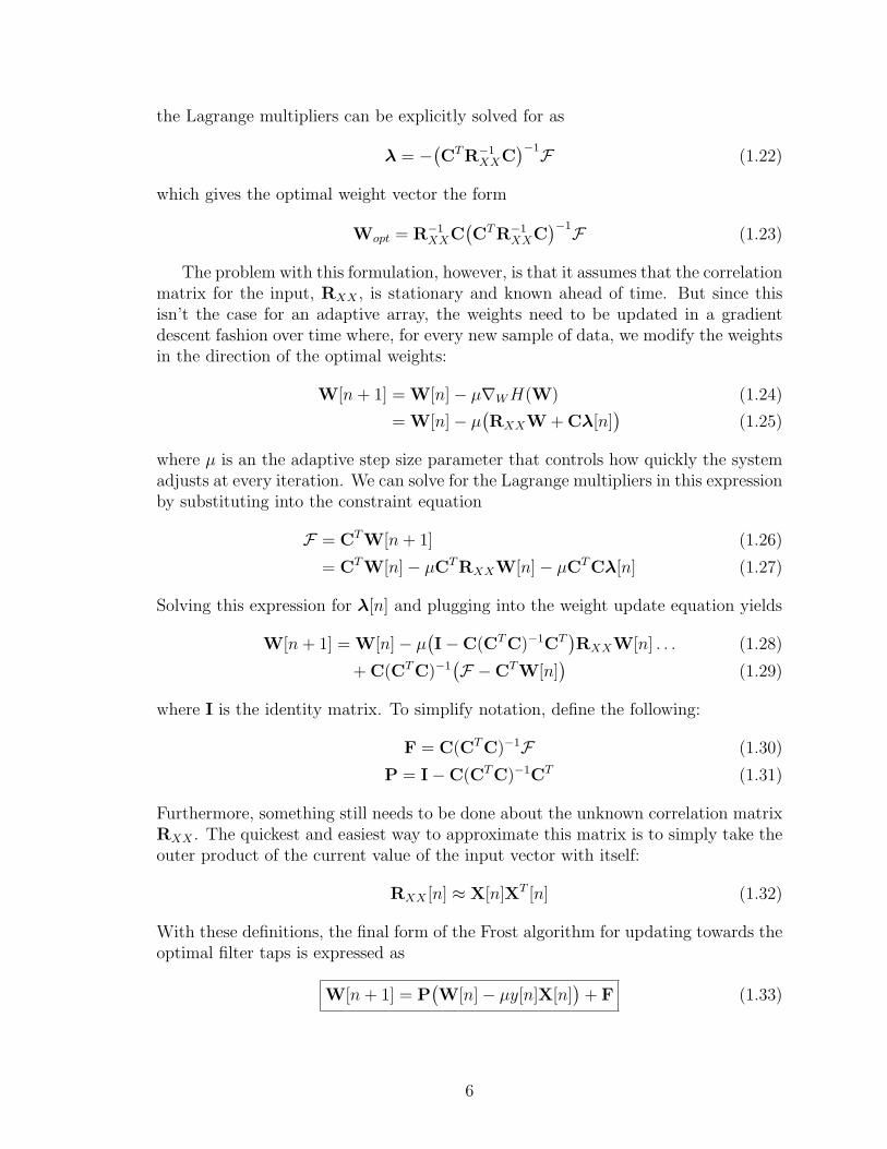
the Lagrange multipliers can be explicitly solved for as

λ = −(

CTR−1XXC

)−1F (1.22)

which gives the optimal weight vector the form

Wopt = R−1XXC

(

CTR−1XXC

)−1F (1.23)

The problem with this formulation, however, is that it assumes that the correlationmatrix for the input, RXX , is stationary and known ahead of time. But since thisisn’t the case for an adaptive array, the weights need to be updated in a gradientdescent fashion over time where, for every new sample of data, we modify the weightsin the direction of the optimal weights:

W[n + 1] = W[n] − µ∇W H(W) (1.24)

= W[n] − µ(

RXXW + Cλ[n])

(1.25)

where µ is an the adaptive step size parameter that controls how quickly the systemadjusts at every iteration. We can solve for the Lagrange multipliers in this expressionby substituting into the constraint equation

F = CTW[n + 1] (1.26)

= CTW[n] − µCTRXXW[n] − µCTCλ[n] (1.27)

Solving this expression for λ[n] and plugging into the weight update equation yields

W[n + 1] = W[n] − µ(

I − C(CTC)−1CT)

RXXW[n] . . . (1.28)

+ C(CTC)−1(

F − CTW[n])

(1.29)

where I is the identity matrix. To simplify notation, define the following:

F = C(CTC)−1F (1.30)

P = I − C(CTC)−1CT (1.31)

Furthermore, something still needs to be done about the unknown correlation matrixRXX . The quickest and easiest way to approximate this matrix is to simply take theouter product of the current value of the input vector with itself:

RXX [n] ≈ X[n]XT [n] (1.32)

With these definitions, the final form of the Frost algorithm for updating towards theoptimal filter taps is expressed as

W[n + 1] = P(

W[n] − µy[n]X[n])

+ F (1.33)

6

1.3.2 The Generalized Sibelobe Canceller (Griffiths-JimBeamformer)

The Generalized Sidelobe Canceller is a simplification of the Frost Algorithm pre-sented by Griffiths and Jim some ten years after Frost’s original paper was published[9]. Displayed in Figure 1.2, the structure consists of an upper branch often called theFixed Beamformer (FBF) and a lower branch consisting of a Blocking Matrix (BM).(Note again that it is assumed that all input channels have already been appropriatelysteered toward the point of interest.)

Figure 1.2: The Generalized Sidelobe Canceller

The upper branch is called a Fixed Beamformer because its behavior is constantover time. The constants wc may be chosen as any nonzero values but are almostalways chosen as simply 1/M , yielding the traditional Delay and Sum beamformer:

yc[n] =1

M

M∑

k=1

xk[n] (1.34)

(Remember that in current notation we assume that the sensors have already beentarget-aligned. In addition, we now adopt the more common practice of referencing

7

the input data and tap weights not as vectors but as matrices of size O × M whereeach column corresponds to data for an individual sensor.) The lower branch utilizesan unconstrained adaptive algorithm on a set of tracks that have passed througha Blocking Matrix (BM), consisting of some algorithm intended to eliminate thetarget signal from the incoming data in order to form a reference of the noise in theroom. The particular BM used by Griffiths and Jim consists of simply taking pairwisedifferences of tracks, which would be visualized for the four-track instance as

Ws =

1 −1 0 00 1 −1 00 0 1 −1

(1.35)

For this Ws the BM output tracks are computed as the matrix product of the blockingmatrix and matrix of current input data.

Z[n] = WsX[n] (1.36)

The overall beamformer output, y[n], is computed as the DSB signal minus the sumof the adaptively-filtered BM tracks

y[n] = yc[n] −M−1∑

k=1

wTk [n]zk[n] (1.37)

where wk[n] is the kth column of the tap weight matrix W of length O and zk[n] isthe kth Blocking Matrix output track, also of length O. The adaptive filters are eachupdated using the Normalized Least Mean Square (NLMS) algorithm with y[n] asthe reference signal

wk[n + 1] = wk[n] + µy[n]zk[n]

||zk[n]||2 (1.38)

A full explanation of how the GSC is derived from the Frost algorithm is beyondthe scope of this work–the most important point is that it arises from ensuring thatthe sum of the weights for the DSB add to 1 and that the constraints for the Frostalgorithm are chosen such that no distortion occurs for the target signal, which foran FIR filter means a digital delta function:

F [n] = δ[n] (1.39)

1.4 Limitations of Current Models and Methods

The greatest problem observed thus far with the GSC is that, if the beamformer isincorrectly steered and doesn’t point perfectly at its target, the target signal won’tbe completely eliminated after it has passed through the blocking matrix [5]. Thisproblem will cause the adaptive filtering and subtracting stage to eliminate not justnoise but some of the target waveform itself from the beamformer output and degradeperformance. Corrections for steering errors have been tackled by some authors pre-viously through the use of adaptive filters using the DSB output as reference [5],

8

though in a noisy environment the improvement will naturally be limited since evenafter the DSB stage the reference signal used will still be corrupted. Instead we pro-pose a different statistical technique to compensate for incorrect steering where inChapter 3 of this thesis we’ll propose and evaluate a cross correlation technique thatattempts to correct the beamformer lags.

In addition, the original formulations of the Frost and Griffiths-Jim algorithmswere based on the general use of beamforming where the far-field assumption is of-ten valid such as in radio astronomy or geology. But in this work, however, we’reconcerned with applying the GSC to an array implemented in an office that is atmost several meters long and wide, meaning that the far field assumption is no longervalid. This change in the physics of the system will also cause leakage in the blockingmatrix with the traditional Griffiths-Jim matrix because now the target signal is nolonger received at each microphone with equal amplitude. Thus in Chapter 2 westudy several amplitude adjustment models that attempt to overcome this problem.

And finally, much of the study of audio beamforming has been carried out withlinear equispaced microphone arrays, due mostly to how arrays of other types ofsensors have been constructed and how simple they are to understand mathematically.However, linear arrays are optimal only for a narrow frequency range that’s dependenton the inter-microphone spacing and can be difficult to construct correctly, especiallyif surveillance is the intended application. Hence Chapter 4 will explore the effectsof microphone geometry on beamforming performance and give guidelines on whatmakes for a good array.

1.5 Intelligibility and the SII Model

In human speech processing it’s customary to evaluate the quality of a speech patternin the presence of noise not in terms of a traditional SNR but a specially weighted scalecalled the Speech Intelligibility Index (SII) [10]. The index is calculated by runningseparate target and interference recordings through a bank of bandpass filters andmultiplying the SNR for each frequency band by a weight based on subjective humantests. The calculation is expressed in notation as

SII =N∑

n=1

AnIn (1.40)

where N is the number of frequency bands under consideration (N = 18 here), An

is the audibility of the nth frequency band (essentially the SNR with some possiblethresholding), and In is the nth frequency band weight. The entire set of weights isreferred to as the Band Importance function and is plotted in Figure 1.3.

The SII parameter ranges from 0 (completely unintelligible) to 1 (perfectly intel-ligible) and is computed over small windows of audio data, traditionally 20ms each,to yield a function of time. In this work the SII will be used to control the initialintelligibility of beamforming tests and provide a model for a simple FIR prefilter thatcan be applied to incoming audio data in order to ensure that the beamformer workssolely on the frequency bands most important to human understanding of speech.

9

0 1000 2000 3000 4000 5000 6000 7000 80000

0.01

0.02

0.03

0.04

0.05

0.06

0.07

0.08

0.09SII Spectrum Weights

Frequency (Hz)

Ban

d Im

port

ance

Figure 1.3: The SII Band Importance Spectrum

1.6 The Audio Data Archive

The experimental evaluations for this thesis are conducted using microphone arraydata collected over several months at the University of Kentucky’s Center for Visu-alization and Virtual Environments. This data archive can be freely accessed overthe World Wide Web [11] where full and up-to-date details on the archive can befound. In short, the data set consists of over a dozen different microphone arraygeometries in an aluminum cage several feet long and wide within a normal officeenvironment. The 16-track recorded WAV files consist of both individual speakers atlaser-measured coordinates and collections of human subjects talking to one anotherin order to simulate a cocktail party scenario, complete with clinking glasses anddishware. The human subjects include both males and females with varying ages andnationalities.

1.7 Organization of Thesis

Chapter 2 studies correcting the amplitude differences between signals entering theGSC Blocking Matrix to provide better target signal suppression by providing sev-

10

eral possible methods to enhance the pairwise subtraction and then evaluating eachmethod over several sets of real audio data. Chapter 3 addresses correcting phaseproblems in the beamformer by using a windowed and thresholded cross correlationtechnique between pairs of tracks and evaluating whether this modification improvesbeamformer quality. Chapter 4 looks at the effects of microphone geometry throughplots of multidimensional beampatterns and parameters for describing DSB beam-field quality. Chapter 5 sums up the research conducted for this work, and finallyAppendix A provides a stability analysis for the GSC using z-transforms and a shortcomputer verification.

11

Chapter 2

Statistical Amplitude Correction

2.1 Introduction

A sine wave at a particular frequency is completely determined by its amplitude andphase, and Fourier theory tells us that any recorded waveform can be viewed as asuperposition of sine waves. Since one of the well-known weaknesses of the traditionalGSC Blocking Matrix (BM) is that target signal leakage will degrade performance,from the Fourier standpoint one has two options to correct this problem: changethe amplitudes in the BM or the phases. In Chapter 3 we address the use of crosscorrelation as a means of optimally estimating the phase difference between receivedtarget signal components, but here we propose and evaluate several techniques fordealing with the amplitude scaling that a sound wave experiences due to propagationthrough air to the microphones and distortion from the recording equipment. Twoof the methods involve using models of the wave physics of the acoustic environmentwhile one other proposes a statistical energy minimization technique in the frequencydomain. In addition, we take advantage of how the audio data set for this thesis hasbeen collected to show a method for simulating a perfect blocking matrix where notarget signal is present whatsoever for comparison. The various methods are thencompared using the correlation coefficient against the closest microphone track to thetarget speaker over many simulated cocktail parties.

2.2 Manipulating Track Order

Before going further, we present one very simple method of combating amplitudechanges that will be utilized in all of our beamformers: switching track order basedon distance.

The original GSC makes no distinctions about the order in which tracks shouldbe processed–in fact, under its original farfield conditions the track order would beirrelevant since the target signal component would always be the same regardlessof microphone-target distance. However, in the nearfield speaker distance will bea significant factor and will, at least in part, cause the target signal component tobe received differently in all microphones. Hence microphones that are at similar

12

1 −1 0 00 1 −1 00 0 1 −1

Figure 2.1: Example Griffiths-Jim Blocking Matrix for a Four-Channel Beamformer

distances to the target speaker will have more similar target components than micsthat have more different distances. Expressed another way

Ak ∝ dk, 1 ≤ k < M (2.1)

Since the goal here is to make the target signal component between pairs of tracksas similar as possible, an easy starting measure is to always sort the track orders andprocess in order from closest to furthest. Hence we force

dk ≤ dk+1∀k (2.2)

This is a small change that, although it may or may not improve the beamform,has virtually zero computational cost as it only involves changing how we index intoour BM tracks after sorting a handful of distances/delays. In addition, some of themodels to be presented will work better if the mic distances are kept in order.

2.3 Models

As discussed in Chapter 1 a major problem with the GSC is leakage of the targetsignal through the Blocking Matrix (BM), causing the adaptive filters to erroneouslyeliminate target components from the overall beamformer output. This is due to theassumption in the algorithm’s original derivation that the microphones receive identi-cal target signals–a valid assumption for the beamformer’s original radar applicationbut not for the realm of nearfield audio beamforming. The original Griffiths-Jimblocking matrix makes this assumption especially conspicuous as it features the pair(1, -1) along the diagonal like in Figure 2.1 [9]. Several authors [5] [12] have addressedthis issue through statistical means with adaptive filtering of blocking matrix chan-nels using the Delay and Sum Beamformer (DSB) component as the reference signal.However, this method will still be prone to target signal leakage since the DSB willtend to achieve only moderate attenuation of at most a few decibels and hence astill-noisy signal will be used as the desired signal for the BM adaptive filters.

In order to attempt to minimize target signal leakage even further we propose andevaluate the following methods.

2.3.1 Spherical Wave Propagation in a Lossless Medium

The basic wave equation in spherical coordinates for an omnidirectional point soundsource without boundaries is [13]

∂p

∂r2+

2

r

∂p

∂r=

1

c2

∂2p

∂t2(2.3)

13

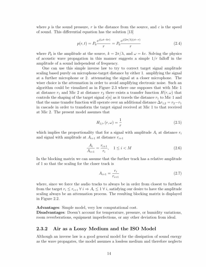
where p is the sound pressure, r is the distance from the source, and c is the speedof sound. This differential equation has the solution [13]

p(r, t) = P0ej(ωt−kr)

r= P0

ej(2π/λ)(ct−r)

r(2.4)

where P0 is the amplitude at the source, k = 2π/λ, and ω = kc. Solving the physicsof acoustic wave propagation in this manner suggests a simple 1/r falloff in theamplitude of a sound independent of frequency.

One can use this simple inverse law to try to correct target signal amplitudescaling based purely on microphone-target distance by either 1. amplifying the signalat a further microphone or 2. attenuating the signal at a closer microphone. Thewiser choice is the attenuation in order to avoid amplifying electronic noise. Such analgorithm could be visualized as in Figure 2.3 where one supposes that with Mic 1at distance r1 and Mic 2 at distance r2 there exists a transfer function H(r, ω) thatcontrols the shaping of the target signal s[n] as it travels the distance r1 to Mic 1 andthat the same transfer function will operate over an additional distance ∆r1,2 = r2−r1

in cascade in order to transform the target signal received at Mic 1 to that receivedat Mic 2. The present model assumes that

H1/r (r, ω) =1

r(2.5)

which implies the proportionality that for a signal with amplitude Ai at distance ri

and signal with amplitude at Ai+1 at distance ri+1

Ai

Ai+1

=ri+1

ri

, 1 ≤ i < M (2.6)

In the blocking matrix we can assume that the further track has a relative amplitudeof 1 so that the scaling for the closer track is

Ai+1 =ri

ri+1

(2.7)

where, since we force the audio tracks to always be in order from closest to furthestfrom the target ri ≤ ri+1 ∀ i ⇒ Ai ≤ 1 ∀ i, satisfying our desire to have the amplitudescaling always be an attenuation process. The resulting blocking matrix is displayedin Figure 2.2.

Advantages: Simple model, very low computational cost.Disadvantages: Doesn’t account for temperature, pressure, or humidity variations,room reverberations, equipment imperfections, or any other deviation from ideal.

2.3.2 Air as a Lossy Medium and the ISO Model

Although an inverse law is a good general model for the dissipation of sound energyas the wave propagates, the model assumes a lossless medium and therefore neglects

14

r1

r2

−1 0 0

0r2

r3

−1 0

0 0r3

r4

−1

Figure 2.2: Blocking Matrix for Spherical Lossless Model

Figure 2.3: Sound Propagation Model as a Cascade of Filters

many of the fluid mechanical losses that a propagating acoustic wave experiencesfrom the effects of viscosity, thermal conduction, and molecular thermal relaxation toname a few [14]. A full treatment of this subject is beyond the scope of this work butthe subject has already been well-researched and the results codified in ISO 9613-1(1993). To summarize, atmospheric sound attenuation is exponentially dependenton the distance the sound travels and a number dubbed the absorption coefficient,αc (dB/m), which is a function of temperature, humidity, atmospheric pressure, andfrequency. The result is a type of lowpass filter of form

Hatm,dB (r, ω, T, P, h) = −rαc(ω, T, P, h) (2.8)

with r in meters, ω = 2πf the radial frequency with f in Hertz, T the temperaturein Kelvin, P the atmospheric pressure in kPa, and h the relative humidity as apercentage. Computation of αc is rather involved but can be quickly and easilyimplemented in software. Since αc is frequency dependent we recognize that usingthe ISO model for a broadband signal amounts to a filtering operation. The frequency

15

Hatm (∆r1,2, ω, T, P, h) −1 0 00 Hatm (∆r2,3, ω, T, P, h) −1 00 0 Hatm (∆r3,4, ω, T, P, h) −1

Figure 2.4: Blocking Matrix for ISO Sound Absorption Model in Frequency Domain

response of this filter can be generated by calculating several values of the absorptioncoefficient for 0 < f < fs/2 and then designing an FIR filter to match the responsedescribed by Eq 2.8. Thus the blocking matrix would be visualized as in Figure 2.4where each closer track is filtered so that its target component matches that receivedat the farther microphone. This method will also result in a pure attenuation process,again ensuring that electronic noise is not unnecessarily amplified.

One potential drawback of this method, even if it’s successful in target signalcancellation, is the fact that the filtering operation on the audio tracks will be appliedto both the target and noise components of the tracks. This operation would thusshape the noise as it enters the MC stage of the beamformer and might present anunnatural change to the system.

Advantages: Very accurate model, uses easily-obtainable information to enhancebeamforming.Disadvantages: Increased computational cost for filtering, and if filter parameterschange the filter design process must be repeated. Temperature, humidity, and at-mospheric pressure must be measured. Doesn’t account for room reverberations orelectronic noise. May add distortion.

2.3.3 Statistical Blocking Matrix Energy Minimization

Though the ISO model takes several more environmental effects into account, by itselfit also fails to consider noise within the electronic equipment, room reverberation, andspeaker directivity. With so many factors affecting how the target sound is changedas it propagates to each of the microphones, we now propose a statistical method foramplitude correction that lumps all the corrupting effects together.

For a pair of real-valued random variables X and Y , it can be shown that if wewish to minimize the the squared error between between two variables using only ascalar multiplication on one, i.e.

(X − αY )2 = e (2.9)

then the constant α that will minimize the energy of the difference e is found as

α =E(XY )

E(Y 2)(2.10)

where E(·) is the expected value operator. If we view the energy minimization problemin time domain where the audio data is always real we’d be done, but the distortions

16

occurring to the target sound has, at least in some part, a frequency dependence. Soinstead, let’s generalize this result to the complex numbers so that a frequency-domainminimization can be carried out. In this case we express the energy as

(X − αY )(X − αY )∗ = e (2.11)

where * denotes complex conjugation. Applying the expected value yields

E

(

(X − αY )(X − αY )∗)

= E(e) (2.12)

E(XX∗) − α(

E(XY ∗) + E(X∗Y ))

+ α2E(Y Y ∗) = E(e) (2.13)

The minimum energy is an extremum for α that can be found by taking the partialderivative with respect to α and solving.

∂

∂α

(

E(XX∗) − α(

E(XY ∗) + E(X∗Y ))

+ α2E(Y Y ∗)

)

=∂

∂α

(

E(e)

)

(2.14)

−(

E(XY ∗) + E(X∗Y ))

+ 2αE(Y Y ∗) = 0 (2.15)

α =12

(

E(XY ∗) + E(X∗Y ))

E(Y Y ∗)(2.16)

This is one possible form of the scaling we wish to use. This expression can berewritten in a more computationally-efficient way by noting that

E(XY ∗) + E(X∗Y ) = 2Re(

E(XY ∗))

(2.17)

andE(Y Y ∗) = E(|Y |2) (2.18)

to get our final result where, since we wish to carry out the operation in frequencydomain, X, Y , and α are all expressed as functions of angular frequency ω

α(ω) =Re(

E(X(ω)Y ∗(ω)))

E(|Y (ω)|2) (2.19)

(Remember again that we assume in our blocking matrix that X and Y have alreadybeen time-aligned to point the beamformer toward the desired focal point, henceno complex exponential phasing is shown.) Using this equation we can calculate acorrection spectrum and apply it to the Fourier transforms of each pair of tracksentering the blocking matrix as

Zk(ω) = Xk(ω) − αk,k+1(ω)Xk+1(ω) (2.20)

Such a blocking matrix is visualized in Figure 2.5. This method will require contin-ually estimating spectra for X(ω) and Y (ω) since these are audio tracks of humanspeech and hence nonstationary. However, voices are slowly-varying enough that if

17

1 −α1,2(ω) 0 00 1 −α2,3(ω) 00 0 1 −α3,4(ω)

Figure 2.5: Statistical Blocking Matrix in Frequency Domain.

we use an averaging technique of several windows on the order of 20ms a good esti-mate of the spectra can be generated. In addition, it’s worthwhile to note that thespectrum computed in Eq 2.19 will be entirely real, meaning that it will target onlythe in-phase components between X(ω) and Y (ω) which should be the target signalcomponents.

Now since we’re forcing all tracks to be maintained in order from closest to furthestfrom the speaker, let’s find a way to choose which of X(ω) and Y (ω) should be thecloser track by analyzing how our statistical filtering will behave if we suppose amakeup of the signals X(ω) and Y (ω) of form

X(ω) = H1(ω)S(ω) + N1(ω) (2.21)

Y (ω) = H2(ω)S(ω) + N2(ω) (2.22)

where we let S(ω) be the target signal spectrum, H1(ω) and H2(ω) be the filters thatshape the target signal components as they travel to the microphones whose signalsare X(ω) and Y (ω), respectively, and N1(ω) and N2(ω) are lumped images of thenoise within X(ω) and Y (ω), respectively. Now to get the target signal completelyeliminated we would want

α(ω) =H1(ω)

H2(ω)(2.23)

To see whether this will happen, we simply plug into Eq 2.16

α(ω) =12

(

E(XY ∗) + E(X∗Y ))

E(Y Y ∗)(2.24)

=

E

(

(

H1(ω)S(ω) + N1(ω))(

H2(ω)S(ω) + N2(ω))∗)

+ . . .

E

(

(

H1(ω)S(ω) + N1(ω))∗(

H2(ω)S(ω) + N2(ω))

)

2E

(

(

H2(ω)S(ω) + N2(ω))(

H2(ω)S(ω) + N2(ω))∗)

(2.25)

To simplify this expression we note that the filters H1(ω) and H2(ω) are deter-ministic and can be taken outside of the expected value and assume that stochasticspectra S(ω), N1(ω), and N2(ω) are all uncorrelated such that an expected value ofany of their products is zero. These considerations will lead to the simplification

α(ω) =Re(

H1(ω)H2(ω))

E(

|S(ω)|2)

|H2(ω)|2E(

|S(ω)|2)

+ E(

|N2(ω)|2) (2.26)

This analysis shows that we should chose Y (ω) as the closer track since the closertrack should tend to have a smaller noise component N2(ω). This discussion also

18

Figure 2.6: GSC Ideal Target Cancellation Simulation Signal Flow Diagram.

shows that, while we should chose Y (ω) as the closer mic between each pair of blockingmatrix tracks, we also realize that the stronger the noise in the closer mic the greaterthe deviation in our correction spectrum from the ideal.

Advantages: Model tailored on the spot to an auditory scene by estimating currentstatistics, thus addressing all acoustic effects at once.Disadvantages: Highest computational cost of the proposed models; correctionspectrum becomes more distorted from ideal as the interference becomes stronger.

2.4 Simulating a Perfect Blocking Matrix

The data sets collected in the UK Vis Center’s audio cage include separate recordingsof individual speakers in a mostly quiet room and cocktail party recordings of severalspeakers. This separation gives us the convenient ability to piece scenarios together bysimply adding together audio files. What we can do with this separation of target andnoise is to feed them separately into the GSC as in Figure 2.6, where now we can trulyobserve a situation where the target signal never flows through the Blocking Matrix.This setup serves the two purposes of providing a benchmark for BM algorithmcomparison as well as showing the ultimate limit on what any BM improvement canprovide for overall GSC enhancement.

19

2.5 Experimental Evaluation

In order to test how well each model performs over many party-speaker positions andmicrophone array geometries, we chose an automated evaluation method using theVis Center Audio Data archive described in Section 1.6. Combinations of a recordingof a lone speaker and a recording of several interfering speakers were created sothat the initial intelligibility [10] of the target speaker could be set to .3 ± .05, avalue considered a threshold for intelligibility. We choose a cross correlation methodbecause:

1. An automated intelligibility test would require that the target and interferencesignals be completely separable, but the behavior of an adaptive system like theGSC is not linear–that is, the adaptation means that

GSC(

s[n] + v[n])

6= GSC(

s[n])

+ GSC(

v[n])

(2.27)

2. A traditional Mean Opinion Score (MOS) test would be very time consuming,especially if we want to gather a large amount of data.

We evaluated both the effectiveness of the blocking matrices and of the overallbeamformers by finding the correlation coefficient with the closest microphone to thelone target speaker, the single best reference of the pure target signal. The correlationcoefficient is computed for random vectors x and y as [15]

ρxy[m] =Rxy[m]

||x||||y|| |ρxy| ≤ 1 (2.28)

where Rxy[m] is the cross correlation between X and Y at lag m, defined as

Rxy[m] =N−m−1∑

n=0

x[n + m]y[n] (2.29)

The normalization by the product of norms for the correlation coefficient ensuresthat ρxy is bounded between -1 and 1. An effective blocking matrix should havea small correlation coefficient (eliminates the target well) while an effective overallbeamformer should have a large correlation coefficient (recreates the target well).The relevant parameters to the beamformer are summarized in Table 2.1 and thecorrelation results displayed in Table 2.3 for the BM and Table 2.2 for the overallbeamformers. Since there were three target speakers and three parties for each ge-ometry the sample size is 9 for each beamformer situation (each of the three speakersgets placed individually into each of the three parties) and hence the sample size foreach BM situation is 135 (nine speaker situations times fifteen BM tracks).

For the statistical energy minimization technique the length of the audio datasegments we use becomes an issue due to the changing statistics of the environment.Here we use different segments of data for spectral estimation and the actual filtering–a shorter segment of data runs through the Blocking Matrix while a longer segment

20

Table 2.1: Parameters for Amplitude Correction Tests

Parameter Value

Number of Microphone Channels M = 16Audio Sampling Rate fs = 22.05 kHz

NLMS Step Size µ = .01NLMS Filter Order O = 32

NLMS Forgetting Factor β = .95Audio Window Length 1024 samples

Spectral Estimation Data Length 4096 samplesSpectral Estimation Window Tukey, r = .25

Closest Mic Initial Intelligibility .3 ± .05ISO Filter Atmospheric Pressure 30 inHg

ISO Filter Temperature 20◦CISO Filter Relative Humidity 40%

including and surrounding the shorter segment is used for power spectral densityestimation associated with the processed segment. Since the FFT runs much fasterwhen the number of points is a power of two, we chose the audio segment length tobe 1024 (about 46ms of audio at fs = 22.05 kHz) and the spectral estimation lengthto be 4096 samples (about 186 ms). For breaking apart the spectral estimation dataa Tukey window was chosen with shape parameter r = .25.

21

2.6 Results and Discussion

The mean correlation coefficients for the overall GSC output with our different BMmodels are displayed in Table 2.2 and as a chart in Figure 2.7. Likewise, the meancorrelation coefficients for the BM tracks using the different models are displayed inTable 2.3 and as a chart in Figure 2.8

Table 2.2: GSC Mean Correlation Coefficients, BM Amplitude Correction

Microphone Geometry

BM Method Linear Rectangular Perimeter Random

Traditional GSC .564 .401 .349 .4671/r Model .565 .396 .347 .461ISO Model .580 .406 .351 .472

Statistical Model .555 .376 .336 .456Perfect BM .631 .426 .376 .503

Table 2.3: BM Track Mean Correlation Coefficient for Various Arrays and Models

Microphone Geometry

BM Method Linear Rectangular Perimeter Random

Traditional GSC .166 .105 .136 .1381/r Model .150 .106 .141 .140ISO Model .176 .137 .153 .157

Statistical Model .215 .185 .175 .207Perfect BM .059 .059 .099 .062

For the Blocking Matrix we notice that, compared to the traditional Griffiths-JimBM, the 1/r model performs slightly worse in all cases and the ISO filtering modelslightly better. Our statistical filtering does a poor job of eliminating the correla-tion with the target signal while, as expected, the perfect BM does very well here.However, changes in BM performance have only a slight effect on overall beamformerperformance, where a difference of as much as 15% in BM correlation improvementtranslates into only a 7% difference in the beamformer output correlation.

22

Figure 2.7: GSC Output Bar Chart for Data in Table 2.2

Figure 2.8: BM Bar Chart for Data in Table 2.3

23

−10 −8 −6 −4 −2 0 2 4 6 8 10

−50

−40

−30

−20

−10

0

f (kHz)

|α(ω

)| (

dB)

Figure 2.9: Sample Magnitude Spectrum for Statistical BM

0 0.1 0.2 0.3 0.4 0.5 0.6 0.7 0.8 0.9 1−2000

−1500

−1000

−500

0

Normalized Frequency (×π rad/sample)

Pha

se (

degr

ees)

0 0.1 0.2 0.3 0.4 0.5 0.6 0.7 0.8 0.9 1−0.7

−0.6

−0.5

−0.4

−0.3

−0.2

−0.1

0

Normalized Frequency (×π rad/sample)

Mag

nitu

de (

dB)

Figure 2.10: Magnitude and Phase Response for ISO Filter, d = 3m

24

To see why the statistical model seems to do so poorly, we present a sample ofthe computed correction spectrum in Figure 2.9. The example shows a very erraticmagnitude response, varying over 50 dB. In contrast, an example of the ISO filteris presented in Figure 2.10 that shows a very smooth frequency response that spansless than one decibel. Since the ISO method works slightly better it would seemthat such an extreme range of filtering as in the Statistical model is not appropriate.This erratic behavior may be due to the fact that, as previously noted, the statisticalmodel performance is expected to deteriorate as the SNR worsens. And, since onewould beamform only in a poor SNR scenario, these results suggest that the statisticalmethod presented in this chapter may, therefore, not be useful at all.

Perhaps the most interesting result is the fact that the BM model used doesnot make as much of a difference as the microphone geometry in each experiment.All cases of the linear array, regardless of BM model, outperform all cases of therandom array, with this pattern continuing in the same manner for the rectangularand perimeter arrays. Listening to some of the sample output tracks (available withthe ETD) makes these statistical results readily apparent–the linear array output issignificantly improved but the differences between the BM models is nearly impossibleto hear save for the perfect BM, while with the perimeter array all models provideonly a small improvement. This reliance on geometry is due to structure of the GSC,where the Delay-Sum portion of the beamformer is influenced only by the arraygeometry, and the results of this chapter indicate that the geometry is, in fact, moreimportant to beamformer performance than any BM technique, even in the best case.In Chapter 4 we’ll carry out an in-depth investigation into what geometries make fora good or bad microphone array.

2.6.1 Example WAV’s Included with ETD

In order to immediately demonstrate the performance of each of the proposed algo-rithms the reader is invited to listen to some sample recordings included with thisETD the List of Files in the front matter of this thesis. Sample WAV’s are providedfor runs on the linear and perimeter arrays for the closest microphone to the tar-get speaker alone, the closest microphone to the speaker in the constructed cocktailparty, and overall GSC output tracks for each of the BM algorithms analyzed in thischapter.

The supplied WAV files should make it clear that, while the perfect blockingmatrix does do slightly better, the different BM algorithms make very little differencein the overall beamformer output where the improvement is dominated by the arraygeometry (the improvement in intelligibility for the linear array is much greater thanfor the perimeter array in all cases).

2.7 Conclusion

In this chapter several methods for suppressing target signal leakage in the GSC BMwere presented and their performance evaluated over several target-noise scenarios

25

for several different array geometries. Using the correlation coefficient against theclosest microphone to the target speaker alone as reference, we determined that, incomparison to the traditional Griffiths-Jim blocking matrix, the 1/r and Statisticalmodels performed slightly worse while the ISO model performed slightly better, bothin terms of target signal leakage in the blocking matrix and overall beamformer per-formance. A theoretical perfect blocking matrix was also run and showed that evenan ideal BM algorithm would be limited in improving the GSC overall.

Copyright c© Phil Townsend, 2009.

26

Chapter 3

Automatic Steering Using CrossCorrelation

3.1 Introduction

Errors in positional measurements for a microphone array are inevitable. Measuredcoordinates for each microphone will suffer whether measured with tape measure orlaser and a target speaker’s mouth will almost never remain in place or, in the caseof surveillance, its position can obviously only be estimated. Chapter 2 addresseshandling target signal leakage in the Blocking Matrix via amplitude adjustments butmakes the assumption that the target position is exactly known, which is practi-cally impossible. However, the cross-correlation is a well-known and highly-robustoperation that can be used between microphone tracks on the fly to estimate the truespeaker position. In this chapter we explain the Generalized Cross Correlation (GCC)procedure as presented in the literature along with a set of proposed improvements:application of bounds on how the much target can move for a windowed correla-tion search, and a threshold on how “certain” the calculations are as the correlationcoefficient before any positional updates are made. We also present a simple multi-lateration technique that can allow for easy retracing from stored TDOA values to anexact Cartesian coordinate for a three-dimensional array. Finally, we fully evaluatehow well the enhanced steering ability improves the overall GSC output.

3.2 The GCC and PHAT Weighting Function

We begin by quickly reviewing the original presentation of the GCC method foroptimally estimating the TDOA of a wavefront over a pair of sensors [16] [17]. Fora pair of microphones n = 1, 2, define the time delays that are required for a waveat some source position to reach each of the sensors as τ1 and τ2 and the TDOAas τ12 = τ2 − τ1. The received signals at the microphones can be expressed in time

27

domain as

x1(t) = s(t − τ1) ∗ g1(qs, t) + v1(t) (3.1)

x2(t) = s(t − τ1 − τ12) ∗ g2(qs, t) + v2(t) (3.2)

(3.3)

which expresses the mic signals as delayed versions of the target signal passed througha filter dependent on space and time combined with some noise. The GCC functionis then defined as the cross correlation of the microphone signal spectra as

R12(τ) =1

2π

∫ ∞

−∞

Ψ12(ω)X1(ω)X2(ω)∗ejωτdω (3.4)

where Ψ12(ω) is a selectable weighting function chosen to make the optimal estimateeasier to detect. This TDOA estimate is chosen as

τ̂12 = argmaxτ∈D

R12(τ) (3.5)

where D is a restricted range of possible delays. One possibility for the weightingfunction that has shown promise is the PHAT (Phase Transform)

Ψ12(ω) =1

|X1(ω)X∗2 (ω)| (3.6)

which has the effect of whitening the signal spectra. This is useful since the correlationoperation shows the greatest peak for white noise which is, optimally, a delta function.

3.3 Proposed Improvements

The use of the GCC method for TDOA estimation in audio beamforming has re-ceived some attention in the literature previously but has been criticized for weakperformance in multi-source and low SNR scenarios [16]. Thus in order to improvethe GCC performance we propose the following modifications:

1. Enforce a criterion on how strong the correlation is between tracks before up-dating, rather than accepting the argmax every time. This should be especiallyhelpful during periods of speaker silence since the argmax would be based purelyon interference.

2. Begin with a seed value for the target speaker location as an explicit Cartesianpoint (sx, sy, sz) and thereafter scan for correlation spikes over a small regionaround the previous focal point rather than the entire room. The smaller theregion we examine, the less of a chance other erroneous correlation spikes willbe detected.

3. Recent research has indicated that restraining the amount of whitening in thePHAT operation may improve localization capabilities [18], so utilize this vari-ant of Ψ12(ω) instead.

We now present our method in full notation.

28

3.3.1 Windowing of Data

First, the method of selecting chunks of audio data over time must be addressedfor two reasons. For one, the length of the audio segments must be chosen shortenough so that the assumption of short-time stationarity for a human voice is valid.In addition, if our algorithm varies the lags used for signal delay between windowsthen discontinuities will occur–if the lags shrink then data will be thrown out and ifthe lags grow then gaps will form. Thus we handle our data windowing as follows:

1. Carry out the algorithm on segments of audio 20ms in length, as is traditionalin audio signal processing.

2. Process the windows with a 50% overlap at the start and combine them at thefinal output with a cosine-squared window. This will smooth-out discontinuitiesformed by changing lags since the cosine-squared window tapers to zero at itsedges where the irregularities would occur.

3.3.2 Partial Whitening

Next, we choose to separate out the PHAT whitening and cross correlation operationsso that the whitening is carried out first in frequency domain but the scan for thecross correlation peak is handled in time domain. Thus we begin by generating thewhitened version of each of the microphone tracks as

x̃k[n] = F−1

{

Xk(ω)

|Xk(ω)|β}

0 < β < 1 (3.7)

where we let the tilde denote the whitened version of xk[n], Xk(ω) is the spectrumof xk[n], and F−1 represents the inverse Fourier Transform. Note that we use thePHAT-β technique of partial whitening [18] by raising the magnitude spectrum inthe denominator to a power less than one. In addition, the whitening spectrum iscomputed with a Hamming window applied in time domain before the FFT is carriedout in order to cut down on ripples in the spectrum from the implied rectangularwindow.

3.3.3 Windowed Cross Correlation

The cross correlation between pairs of microphone tracks is then carried out on thewhitened signals as

R(i)k,k+1[n] = x̃

(i)k ⋆ x̃

(i)k+1 1 ≤ k < M (3.8)

=

ξ=τ(i)k,k+1+D∑

ξ=τ(i)k,k+1−D

x̃(i)k [ξ]x̃

(i)k+1[n + ξ] (3.9)

where the superscript (i) indicates the number of the data window being processed(usually of length 20ms), ξ is the dummy variable of cross correlation, τk,k+1 is the

29

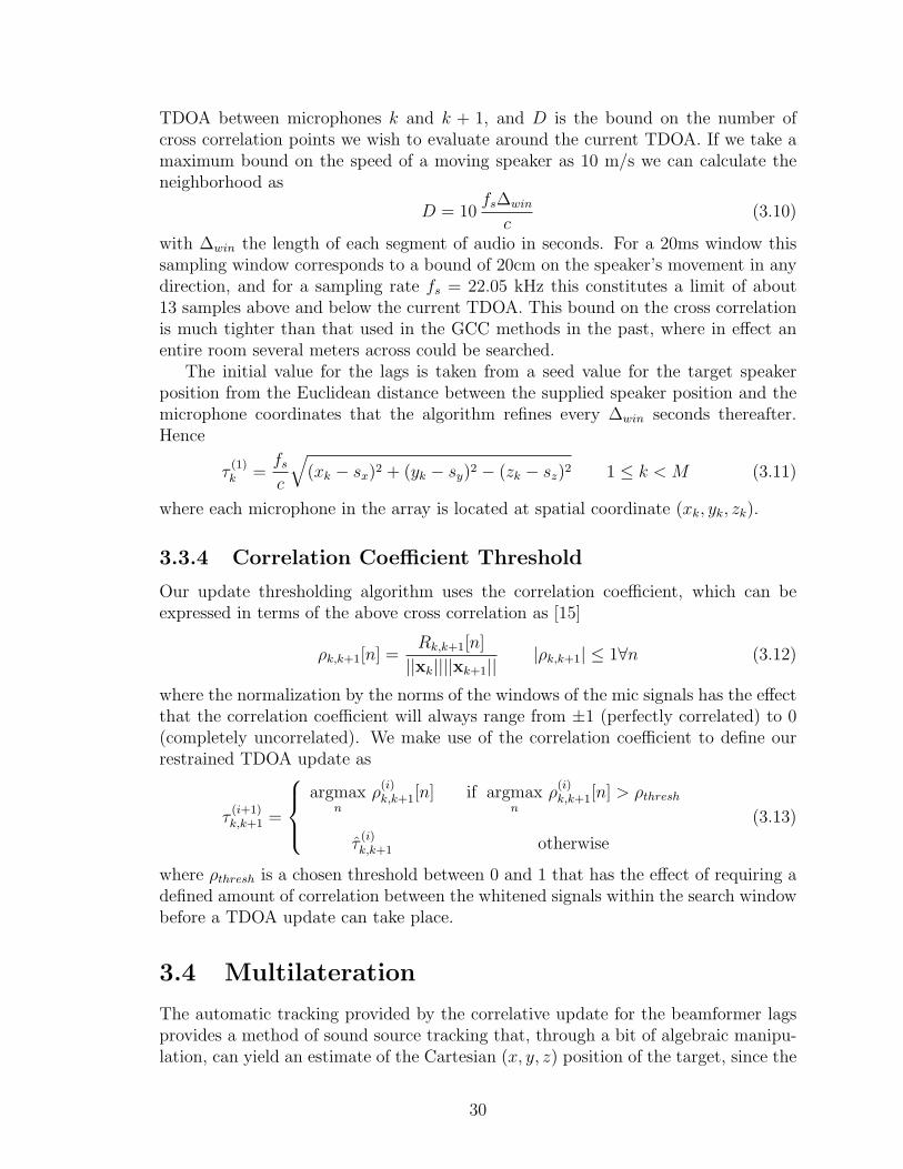
TDOA between microphones k and k + 1, and D is the bound on the number ofcross correlation points we wish to evaluate around the current TDOA. If we take amaximum bound on the speed of a moving speaker as 10 m/s we can calculate theneighborhood as

D = 10fs∆win

c(3.10)

with ∆win the length of each segment of audio in seconds. For a 20ms window thissampling window corresponds to a bound of 20cm on the speaker’s movement in anydirection, and for a sampling rate fs = 22.05 kHz this constitutes a limit of about13 samples above and below the current TDOA. This bound on the cross correlationis much tighter than that used in the GCC methods in the past, where in effect anentire room several meters across could be searched.

The initial value for the lags is taken from a seed value for the target speakerposition from the Euclidean distance between the supplied speaker position and themicrophone coordinates that the algorithm refines every ∆win seconds thereafter.Hence

τ(1)k =

fs

c

√

(xk − sx)2 + (yk − sy)2 − (zk − sz)2 1 ≤ k < M (3.11)

where each microphone in the array is located at spatial coordinate (xk, yk, zk).

3.3.4 Correlation Coefficient Threshold

Our update thresholding algorithm uses the correlation coefficient, which can beexpressed in terms of the above cross correlation as [15]

ρk,k+1[n] =Rk,k+1[n]

||xk||||xk+1|||ρk,k+1| ≤ 1∀n (3.12)

where the normalization by the norms of the windows of the mic signals has the effectthat the correlation coefficient will always range from ±1 (perfectly correlated) to 0(completely uncorrelated). We make use of the correlation coefficient to define ourrestrained TDOA update as

τ(i+1)k,k+1 =

argmaxn

ρ(i)k,k+1[n] if argmax

nρ

(i)k,k+1[n] > ρthresh

τ̂(i)k,k+1 otherwise

(3.13)

where ρthresh is a chosen threshold between 0 and 1 that has the effect of requiring adefined amount of correlation between the whitened signals within the search windowbefore a TDOA update can take place.

3.4 Multilateration

The automatic tracking provided by the correlative update for the beamformer lagsprovides a method of sound source tracking that, through a bit of algebraic manipu-lation, can yield an estimate of the Cartesian (x, y, z) position of the target, since the

30

number of lags required for a sound to reach a microphone is directly proportional tothe Euclidean distance. In R

3 any combination of three distances would uniquely de-termine the position of the target, but since in general M > 3 for a microphone arraywe are presented with an overdetermined system since more information is providedthan there are parameters to be determined. However, this extra information overthe array allows us to make a calculation over the entire array that minimizes theerror over all sets of lags in the least-squares sense. This multilateration algorithmprovides a very efficient method for sound source location and is derived as follows:

Suppose that the positions of the M microphones in an array are precisely knownin R

3, denoted as (x1, y1, z1), (x2, y2, z2), ..., (xM , yM , zM), and that the lags for abeamform for speed of sound c and sampling rate fs are also known as τ1...M . Wewish to solve for the position of the target (sx, sy, sz). Firstly, the distances from eachmicrophone to the target follow directly from the lags as

τi = difs

c1 ≤ i ≤ M (3.14)

Each of these distances is related the positions of the ith microphone to the sourceby the formula for Euclidean distance

di =√

(xi − sx)2 + (yi − sy)2 + (zi − sz)2 1 ≤ i ≤ M (3.15)

or, by squaring both sides

d2i = (xi − sx)

2 + (yi − sy)2 + (zi − sz)

2 1 ≤ i ≤ M (3.16)

Now what we would like to do is formulate a system of equations using thesedistance relationships that would allow us to solve for (sx, sy, sz), but in the presentform the squared terms for the source position are problematic if we wish to takea linear algebra route. However, those terms can be eliminated by expanding andtaking differences of equations. If we expand Eq (3.16) and write the terms for boththe i and i + 1 case we have

x2i − 2xisx + s2

x + y2i − 2yisy + s2

y + z2i − 2zisx + s2

z = d2i (3.17)

x2i+1 − 2xi+1sx + s2

x + y2i+1 − 2yi+1sy + s2

y + z2i+1 − 2zi+1sx + s2

z = d2i+1 (3.18)

If we subtract the second line from the first, the squared terms for the sourceposition disappear:

x2i −x2

i+1−2sx(xi−xi+1)+y2i −y2

i+1−2sy(yi−yi+1)+z2i −z2

i+1+2sz(zi−zi+1) = d2i −d2

i+1

(3.19)Now we can rearrange this equation so that only terms involving the target posi-

tion are on one side as

2sx(xi+1 − xi) + 2sy(yi+1 − yi) + 2sz(zi+1 − zi) = ... (3.20)

d2i − d2

i+1 + x2i+1 − x2

i + y2i+1 − y2

i + z2i+1 − z2

i (3.21)

31

Notice that all terms on the righthand side are known ahead of time. For theM −1 differences in distance that can be calculated we can write out Eq (3.20) M −1times. In matrix form this would be

2

x2 − x1 y2 − y1 z2 − z1

x3 − x2 y3 − y2 z3 − z2...

......

xM − xM−1 yM − yM−1 zM − zM−1

sx

sy

sz

=

d21 − d2

2 + x22 − x2

1 + y22 − y2

1 + z22 − z2

1

d22 − d2

3 + x23 − x2

2 + y23 − y2

2 + z23 − z2

2...

d2M−1 − d2

M + x2M − x2

M−1 + y2M − y2

M−1 + z2M − z2

M−1

(3.22)

where the matrix dimensions are (M − 1× 3), (3× 1), and (M − 1× 1), respectively.Now we can use the simple fact from linear algebra that, for an overdetermined systemof form Ax = b, the least squares solution of the system is found as

x = (ATA)−1ATb (3.23)

If we let A be the first matrix of Eq (3.22), x be the middle vector, and b be thefinal vector, then the position vector of the target can be solved for using Eq (3.23).

Though this algorithm requires a seed value for target position since it uses thelags from the modified GSC, its automatic tracking ability is a very attractive featureversus sound source location (SSL) schemes that essentially require beamforming overmany points through some volume of space per every timeframe of audio. Correlationand multilateration, however, are fast operations that need to be run only once perframe of audio data and thus have the potential for great computational savings.

One interesting limitation of this algorithm is that its ability to find a targetposition can be limited by the geometry of the array for the special cases of planarand linear microphone arrays. For the case of a planar array the z-coordinate of allmicrophones will be the same, thus forcing the rightmost column of the first matrixin Eq (3.22) to be zero. But if we attempt to solve using (3.23) the inverse of A willnot exist since A will be rank-deficient (rank at most 2 for an M − 1 × 3 matrix).

3.5 Experimental Evaluation

3.5.1 GSC Performance with Automatic Steering

To evaluate how the cross correlation updates for the array steering lags affect GSCperformance, we repeated the correlation comparison technique used for evaluationin Chapter 2 where the speaker intelligibility was set to around .3 and the correla-tion coefficient was found between the beamformer output and the closest mic to the

32

Table 3.1: GSC Mean Correlation Coefficients, Automatic Steering

Microphone Geometry

ρthresh Linear Rectangular Perimeter Random

.1 .494 .280 .324 .399

.2 .526 .298 .329 .403

.3 .527 .288 .332 .410

.4 .513 .339 .341 .409

.5 .523 .376 .347 .428

.6 .531 .389 .347 .442

.7 .547 .398 .347 .458

.8 .552 .402 .347 .459

.9 .561 .402 .347 .463

Table 3.2: BM Mean Correlation Coefficients, Automatic Steering

Microphone Geometry

ρthresh Linear Rectangular Perimeter Random

.1 .210 .131 .174 .173

.2 .210 .131 .169 .169

.3 .208 .130 .169 .168

.4 .204 .128 .167 .165

.5 .200 .127 .166 .164

.6 .198 .126 .166 .164

.7 .197 .126 .166 .164

.8 .197 .125 .166 .164

.9 .196 .125 .166 .163

target speaker. (Refer back to Table 2.1 for system parameters). Since the choiceof amplitude correction method made little difference in Chapter 2 the simplest ap-proach, the traditional Griffiths-Jim pairwise subtraction, is used. The parameterρthresh was chosen to vary from .1 to .9 and again the correlation between the targetsignal and both the BM tracks and overall GSC output was measured. The resultsare displayed in Tables 3.1 and 3.2 and visualized in Figures 3.1 and 3.2 for the GSCoutput and BM tracks, respectively.

3.5.2 Multilateration Versus SRP

The multilateration technique presented in this work requires a fully three-dimensionalarray in order to find a least-squares coordinate in R

3. Of the arrays in the UK VisCenter Data Archive, three fit into this category (all others are either 2D or linear).

33

Figure 3.1: Bar Chart of GSC Output Track Correlations w/ Target

The data archive includes target speaker positions calculated by the SRP-PHATsound source location technique [19]. For each of these arrays, we chose to run multi-lateration on the lags calculated by the thresholded cross correlation for ρthresh = .1,to .9 by increments of .1 and then calculate the mean Euclidean distance between thecalculated points as

e =1

Npts

Npts∑

i=1

√

(xi,M − xi,SSL)2 + (yi,M − yi,SSL)2 + (zi,M − zi,SSL)2 (3.24)

where Npts is the number of points that SSL calculated over the entire audio track.Npts may not and usually doesn’t equal the number of 20 ms windows for the entiretrack since the SSL technique won’t always detect a target speaker, especially whenthe talker is silent. We find this mean distance and the beamformer output correlationwith the closest mic track to the target speaker alone as we again vary the correlationthreshold from .1 to .9. The results are displayed in Tables 3.3 and 3.4 for the outputcorrelations and errors, respectively, and visualized in Figures 3.3 and 3.4.

34

Figure 3.2: Bar Chart of BM Output Track Correlations w/ Target

Table 3.3: Beamformer Output Correlations for Various Thresholds

Microphone Geometry

ρthresh Endfire Cluster Pairwise Even 3D Spread Cluster

.10 .2190 .2420 .238

.20 .2530 .2550 .280

.30 .2560 .2960 .273

.40 .2720 .3320 .280

.50 .2720 .3620 .294

.60 .2800 .3660 .302

.70 .2780 .3620 .307

.80 .2770 .3790 .320

.90 .2760 .3820 .318

35

Table 3.4: Mean Multilateration Errors vs SSL for Various Thresholds

Microphone Geometry

ρthresh Endfire Cluster Pairwise Even 3D Spread Cluster

.1 3.625 1.444 0.285

.2 5.654 1.587 1.290

.3 5.578 1.599 1.263

.4 5.651 1.591 1.344

.5 5.888 1.571 1.367

.6 6.132 1.571 1.364

.7 6.173 1.573 1.366

.8 6.174 1.570 1.371

.9 6.192 1.570 1.368

Figure 3.3: Bar Chart of Correlations from Table 3.3

36

Figure 3.4: Bar Chart of Mean Errors vs SSL from Table 3.4

3.6 Results and Discussion

Since the target speaker has been held stationary for all recordings in the data archive,we expect that the only improvements for target steering would come from very smalladjustments accounting for the tiny movements of a person’s body as he speaks.Given this fact, we would expect a very high correlation coefficient threshold to beappropriate, and as Tables 3.1 and 3.2 show this is certainly the case. In fact, theresults for the four arrays as used in Chapter 2 seem to suggest that the only goodscenario, given that it’s known the target is still, is to use no updating at all. Thisfact again shows the difficulty of using statistical methods in an inherently poor SNRsituation.

In order to further investigate the correlation scheme’s performance we examinethe results of the multilateration tests, which will allow us to see a fully 3D renderingof where the beamformer “thinks” the target is at some instant. The results aredisplayed in Tables 3.3 and 3.4 and visualized in Figures 3.3 and 3.4.

What’s interesting to see here is that the mean error between multilaterion overthe adjusted lags and SSL doesn’t change a great deal as the threshold for updatingthe alignment lags increases. To see why this is so, we take a look at some sampleplots for the Endfire Cluster array of both the multilateration versus SSL points andthe raw lags in the beamformer for thresholds of .1, .5, and .9. The points are plottedin Figures 3.5, 3.6, and 3.7 and the lags in Figures 3.8, 3.9, and 3.10.

37

0.51

1.52

2.53

1

2

3

−5

0

5

x (m)y (m)

z (m

)

MicrophonesMultilaterationSSL

Figure 3.5: Multilateration and SSL Target Positions, ρthresh = .1

0.51

1.52

2.53

1

2

3

1.5

2

2.5

3

x (m)y (m)

z (m

)



The positional plots show that the thresholding is working to some degree–the

38

0.51

1.52

2.53

1

2

3

1.5

2

2.5

3

x (m)y (m)

z (m

)



200 400 600 800 1000 1200

40

60

80

100

120

140

160

180

200

220

Window number

DS

B C

hann

el L

ag


higher that threshold, the less often the focal point of the array will shift. For a low

39

200 400 600 800 1000 1200

60

80

100

120

140

160

180

200

220

Window number

DS

B C

hann

el L

ag


200 400 600 800 1000 1200

100

120

140

160

180

200

220

Window number

DS

B C

hann

el L

ag


threshold like .1 the focal point moves very often and rather erratically, even moving

40

beyond the bounds of the room, while for a high threshold like .9 there are very fewadjustments. At the same time, we notice that the low threshold plot indicates anability to return to the correct focal point even after a large misadjustment sincethere are many points clustered around the SSL points as well as far away. On theother hand, the small number of points for the high threshold plot indicate that whilea bad adjustment may be rare, undoing a bad adjustment is also as rare. These factsseem to indicate a potential tradeoff between low and high correlation thresholds:a low threshold is more likely to go off track but can recover more easily, while ahigh threshold is less likely to readjust incorrectly but has a far more difficult timerecovering if it does.

The most revealing result of the Multilateration plots is that, despite our limita-tion that the target can move no more than 20cm in a 20ms time frame, we noticein Figure 3.7 that the least squares retraced focal point can jump by as much as ameter over a single frame. This fact suggests that enforcing a much smaller windowon the correlation may help, perhaps because the 20cm window is enforced on eachpair of tracks and not the entire array, meaning that in the worst case the distancelimit compounds.

Finally, it’s again worth mentioning that all audio data analyzed from the VisCenter archive involves stationary targets and interferers, which may give an unfairbias towards never adjusting the focal point. An interesting piece of future workwould be be an investigation of how the presented tracking scheme would behave fora moving target speaker and how it would perform against SSL, especially when thetarget speaker has longer periods of silence as he moves. This would likely require anenlarged search window or other criteria for correct tracking.

3.6.1 Example WAV’s Included with ETD

Like in Chapter 2, a collection of sample WAV files for the results of the correlationtechnique presented in this chapter has been provided. The samples are for the lineararray setup as in Chapter 2 with the same speaker and noise environment and theupdate threshold chosen for .1, .5, and .9. These files should help demonstrate thatthe looser thresholds show erratic and quickly degrading performance while the higherthreshold, although initially ensuring a good beamform, eventually begins to breakdown as well. In all cases, it should be clear that, compared to the beamformeroutput of the traditional GSC as in the included files for Chapter 2, the correlationtechnique is never as effective.

3.7 Conclusion

In this chapter a method for automatically adjusting the focal point of a beamformerby updating a seed value using a cross correlation technique was presented alongwith a least-squares method of estimating the focal point of a three-dimensional arraygiven its alignment lags. Results indicate a worsening of performance for all examinedscenarios with a steady decline in all cases as the correlation coefficient threshold is

41

reduced. These results may be due to a bias caused by target and competing speakersnever moving and too large of a correlation search window, but may also point towardthe general idea that statistical methods may always face serious difficulties underpoor SNR conditions.

Copyright c© Phil Townsend, 2009.

42

Chapter 4

Microphone Geometry

4.1 Introduction

In Chapter 1 is was shown that the GSC results from the factoring of the Frost algo-rithm for an optimal beamformer into two portions: a fixed Delay-Sum Beamformerand an adaptive stage called the Blocking Matrix (BM). Given the fact that resultsfrom Chapters 2 and 3 show a clear limit to how much improvement can be realizedby improving the adaptive stage, we now turn our attention to the Delay-Sum Beam-former whose performance can be modified only by changing the array geometry.Since equispaced linear arrays are limited in their voice capture capabilities in thischapter we evaluate more general array geometries in two and three dimensions. Webegin by introducing visualization of the beamfields with volumetric plots, then goon to analyze stochastic arrays in the general sense through Monte Carlo simulationsusing a set of proposed evaluation parameters and compare the performance of theirregular arrays to that of a regular rectangular array. Finally we conclude with someguidelines for optimal microphone placement.

4.2 Limitations of an Equispaced Linear Array

The traditional equispaced linear array suffers from three significant problems. Thefirst is that its regular spacing makes it useful only for a narrow range of frequencies.The strongest condition on this range is spatial aliasing, the analog of the Nyquistrate for beamforming which states [4]

d <λmin

2(4.1)

for intermic spacing d. However, the optimal intermic spacing range for a lineararray tends to be tighter because as waves are shifted and added together in theDSB both extremes of a relatively long wavelength (not enough change in the shiftoperation) and relatively short wavelength (too much change in the shift operation)are undesirable. Unfortunately, human speech is an inherently very wideband signalwith significant components ranging from 50-8000 Hz [10], indicating that an arraytuned to a single frequency will have a far smaller effective bandwidth than necessary.

43

The second limitation is the fact that an equispaced linear array is steered usingonly a single parameter θ, the angle of incidence of the target wavefront with respectto the array’s axis. This type of steering means that sound sources that are colinearwith respect to the array steering cannot be resolved. In addition, the rotationalsymmetry of the array means that sounds at different heights for a horizontal arraycannot be resolved, either.

The third limitation is the fact that under many circumstances an equispacedlinear array may not be feasible to construct. For example, in the case of a smartroom such as that constructed in the AVA Lab (Ambient Virtual Assistant) at theUniversity of Kentucky Visualization Center, microphones placed in a ceiling aresubject to placement constraints such as lighting, ventilation systems, or the metalceiling tile grid. In the case of a surveillance system an array may need to be placedtoo quickly and discreetly for precise intermic spacings to be enforced. And evenin the event that an equispaced linear array can be constructed precise microphoneplacement can be very difficult to achieve even with laser systems [20].

Thus in light of these issues, we now wish to analyze arrays of more generalgeometries to see what layouts might work better for human voice capture. We beginby studying the plot of the sound power that a beamformer picks up as a function ofposition in space, called the beampattern.

4.3 Generating and Visualizing 3D Beampatterns

The response of a linear array as a function of steering angle is a one-dimensionalfunction of θ, but if we generalize the array and its steering capability to R

3 thenwe face the challenge of generating a volumetric plot–a visualization of a functionof three variables. Here we wish to plot the beamformer power as a function of aCartesian (x, y, z) coordinate.

Since human perception can understand only three spatial coordinates, we chooseto use color as our fourth dimension in the plots. Here we choose to use the classic Jetcolormap which renders the weakest intensities in blue and then progresses to green,yellow, orange, and finally red for the strongest intensities. In addition, we recognizethat our rendering will require the ability to see into a volume, since areas of lowintensity will wrap around areas of high intensity and may obscure our view if greatcare is not taken. For that our solution is to use an intensity-dependent transparencythat renders the weak areas lightly (very transparent) and the strong areas heavily(nearly opaque).

The plots are generated by propagating a burst of noise colored to match theSII spectrum onto an array of microphones using a sound simulator software andevaluating the beamformer response throughout some volume of interest. Since thebeamfield must naturally be evaluated at only a discreet number of points, we choosethe beamfield resolution as

∆grid =.4422c

fmax

√d

(4.2)

where d is the dimension of the grid space (3 for a volumetric plot) and fmax is the

44

greatest frequency of the target sound. This choice of spacing ensures that no morethan a 3 dB change in the beamfield will occur between grid points [19].

The operations of holding a sound source stationary and sweeping the array focalpoint and holding the focal point stationary and sweeping the sound source positionare equivalent operations for generating the DSB beamfield in a small room where,as shown in Chapter 2, sound attenuation through air has a negligible effect overonly a couple meters (.6 dB at the highest frequencies, which is significantly smallerthan the 3dB threshold of variation for the grid spacing). To see this, consider thefact that for a source at point a = (ax, ay, az) the simulated signal x[n] at the ith

microphone with position (xi, yi, zi) will be

xi[n] = x[n − τa] (4.3)

where

τa =fs

c

√

(xi − ax)2 + (yi − ay)2 + (zi − az)2 (4.4)

and that the delay applied in the DSB operation to find the power at point b =(bx, by, bz) is

τ2 =fs

c

√

(xi − bx)2 + (yi − by)2 + (zi − bz)2 (4.5)

Thus the DSB computes

y[n] =1

M

M∑

i=1

xi[n − τb] (4.6)

=1

M

M∑

i=1

x[n − τa − τb] (4.7)

where clearly the order of delays is irrelevant. This choice in the order of operationsis significant because it allows us to run the sound simulator only once rather than atevery grid point in the volume of interest, which is a very time consuming operation.(For the current Matlab implementation, this reversal can make the difference ofthirty minutes of processing spread out over computer cluster versus ten minutes ona single PC.)

4.4 A Collection of Geometries

In Section 4.3 we outlined our algorithm for visualizing beampatterns in three dimen-sions. We now display the beampatterns for several of the office setting microphonearrays from the Vis Center data archive for specified focal points in order to gainsome insight into what makes for an effective array and what doesn’t. Note that allthe arrays except for Random Array 1 have the same intensity colorbar scale rangingfrom -2 to -12 dB below the focal point maximum and that the microphone positionsare overlaid as gray dots. Also note that there is no single beampattern for an array(the farfield linear array is the single exception), but as will be shown in the Monte

45

Carlo experiment the beamfield generated for a source point below the center of thearray will be the best case scenario and that array performance should always degradefor all other focal points.

4.4.1 One Dimensional Arrays

4.4.1.1 Linear Array

Figure 4.1: Linear Array Beamfield, Bird’s Eye View

The linear array, for as much as it’s been criticized so far, performs rather wellcomparatively. Because of the nearfield nature of the array and the fact that thebeamfield isn’t viewed as a function of angle the traditional sinc pattern isn’t readilyapparent. One may argue, however, that this fact is an advantage of a linear arrayin an office environment where the large aperture size of the array relative to theenclosure means that sidelobes will rarely fit inside the room. Notice also that themainlobe is clearly elongated in the direction of the array and the rotational symmetryof the beampattern in the perspective view. The perspective view of this beampatternis one of several that demonstrates that assuming zero variance in the beamfield withrespect to z is a reasonable approximation.

46

Figure 4.2: Linear Array Beamfield, Perspective View

4.4.2 Two Dimensional Arrays

4.4.2.1 Rectangular Array

The rectangular array has a tighter mainlobe than the linear array, but the bird’s eyeview shows that the sidelobes are more prominent and radiate out from the mainlobemuch further than for the linear array. While the beampattern varies somewhat withheight the features show only slow variation in the z direction.

4.4.2.2 Perimeter Array

The perimeter array does a very good job of keeping a tight mainlobe along withnearly uniform suppression everywhere else in the room. There’s also very littlevariance of intensity with height.

47

Figure 4.3: Rectangular Array Beamfield, Bird’s Eye View

Figure 4.4: Rectangular Array Beamfield, Perspective View

48

Figure 4.5: Perimeter Array Beamfield, Bird’s Eye View

Figure 4.6: Perimeter Array Beamfield, Perspective View

49

4.4.2.3 Random Ceiling Array 1

Figure 4.7: First Random Array Beamfield, Bird’s Eye View

Figure 4.8: First Random Array Beamfield, Perspective View

50

This first random array (the one used in the experiments in Chapters 2 and 3)has the strongest DSB beampattern of all the arrays to be considered in this section.Outside its mainlobe the suppression is so strong that the color scale has to rangedown to -20 dB to pick it up (as opposed to -12 dB for all the others). Again, notethe small variation in the z direction.

4.4.2.4 Random Ceiling Array 2

Figure 4.9: Second Random Array Beamfield, Bird’s Eye View

This second random array does well to demonstrate that “random” doesn’t nec-essarily mean “effective”. This array performs by far the worst out of all thoseconsidered, where on average the signal suppression outside the mainlobe is hardlybetter than -8 dB when nearly all others get down to at least -12 dB. The two randomarrays presented here demonstrate that while an irregularly-spaced microphone arrayshows great potential more work must be done in order to quantify what it is aboutthe “randomness” that translates into better performance.

4.4.3 Three Dimensional Arrays

4.4.3.1 Corner Cluster

The corner cluster array illustrates the extreme form of what happens when an arrayhas a small aperture size and is heavily lopsided away from its target (subjects tobe addressed more formally in the next section). The main lobe of the array is bothvery wide and elongated.

51

Figure 4.10: Second Random Array Beamfield, Perspective View

Figure 4.11: Corner Array Beamfield, Bird’s Eye View

52

Figure 4.12: Corner Array Beamfield, Perspective View

Figure 4.13: Endfire Cluster Beamfield, Bird’s Eye View

53

Figure 4.14: Endfire Cluster Beamfield, Perspective View

4.4.3.2 Endfire Cluster

The idea behind the endfire cluster array was to attempt to design an array withclusters of microphones with small intermic spacings that would be optimal for beam-forming at high frequencies and then spread the clusters out so that between clustersthe beamformer would also be optimized for low frequencies. This hypothesis turnsout to be incorrect as one examines the beamfield, where although the mainlobe isvery tight sidelobes are very strong and suppression is generally very bad throughoutthe room.

It’s also worth pointing out that although the endfire cluster array is technically3D the variation in z of its mic positions is small, hence the small variance of itsbeamfield in the z direction.

4.4.3.3 Pairwise Even 3D Array

The pairwise array is another example of how combining strictly closely and looselyspaced microphones is ineffective at achieving good interference suppression for theDSB. Virtually an entire quarter of the room is part of the mainlobe in these plots.

4.4.3.4 Spread Cluster Array

This array again shows that an irregular array has just as much of a chance of per-forming poorly as performing well.

54

Figure 4.15: Pairwise Even 3D Beamfield, Bird’s Eye View

Figure 4.16: Pairwise Even 3D Beamfield, Perspective View

55

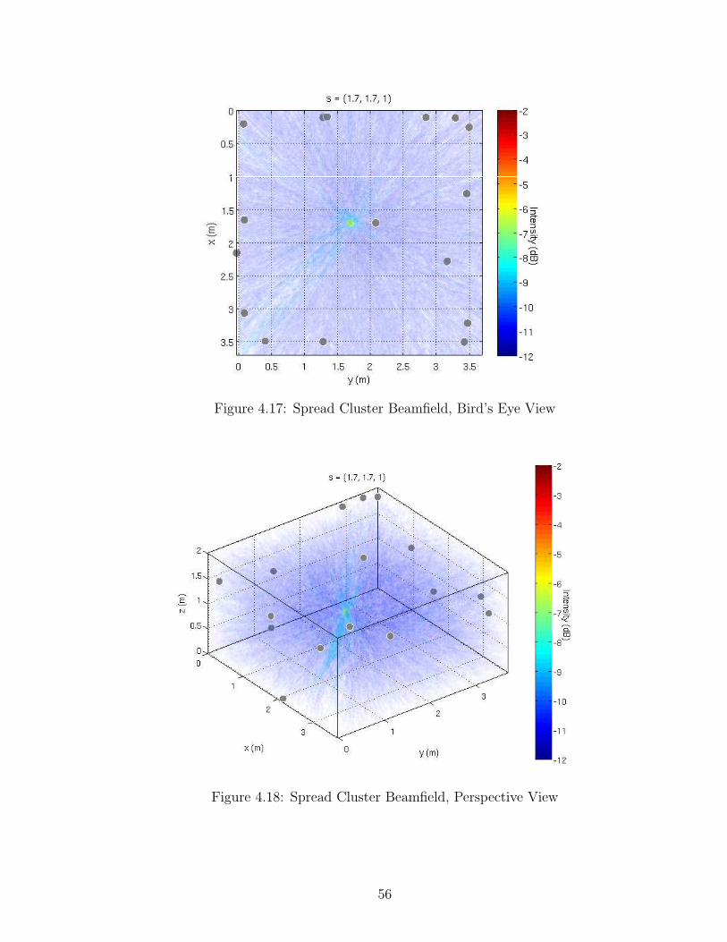
Figure 4.17: Spread Cluster Beamfield, Bird’s Eye View

Figure 4.18: Spread Cluster Beamfield, Perspective View

56

4.4.4 Comparison of Beamfields to Earlier ExperimentalResults

Now that we have some ability to visualize the DSB beampatterns of the arrays in thedata archive, we now compare these plots to the results of Chapters 2 and 3, wherealmost regardless of algorithm the order of array performance from best to worst was:

1. Linear

2. Random Array 1

3. Rectangular

4. Perimeter

The beamfields presented somewhat agree with this list: the random array shouldbe toward the top of the list and the rectangular toward the bottom. But frombeamfields alone we’d expect the perimeter array to beat out the rectangular and therandom array to be the best of all, especiallly over the linear array. Three potentialexplanations for this outcome are:

1. The locations of the target speakers in all tests was well known via Sound SourceLocation (SSL) but no localization was carried out for the interfering cocktailparty recordings. This means that some tests may have been biased towardcertain arrays and against others where the sidelobes of an array never hadinterferers in one experiment but did have them in another. Although the dataset used was moderately large the confounding effect may have been signficant.This would be rectified in the data set by forcing all target positions to bemeasured.

2. The relative performance of the Delay-Sum beamformer in the GSC to theblocking matrix was not assessed. Notice that in the results of Chapter 2 thatthe Linear array had the best GSC output but also the most leakage in theBM. Since the DSB and BM must work together in the GSC evaluating theirrelative performance would likely reveal a great deal about array performance,but this analysis is left as future work.

3. The algorithm used for generating the beampatterns made the assumptionsthat the attenuation of sound through air was negligible and that there wasno reverberation at the room boudnaries, both of which may practically beincorrect. More thorough simulation may rectify this potential problem, butthe processing time required to generate plots would be very long.

57

4.5 A Monte Carlo Experiment for Analysis of

Geometry

4.5.1 Proposed Parameters

In addition to our more qualitative analysis of visually inspecting and judging beam-patterns we’d like to have a quantitative way to compare them, especially if we’d liketo compare lots of arrays statistically. Since we’ve seen that a two-dimensional arraycan behave as well as a fully 3D one and can be constructed more easily, followingparameters for characterization of a 2D beamfield are proposed:

• Main Lobe Width (MLW) - The 3 dB width of the main lobe, calculatedfrom the x and y 3 dB widths using

w3dB =√

x23dB + y2

3dB (4.8)

• Peak to Sidelobe Ratio (PSR) - The difference between the mainlobe andgreatest sidelobe powers in decibels

PSRdB = Pmain − Psl (4.9)

The MLW is a measure of the beamform resolution, and the PSR is a measure of theworst-case leakage of noise from other sources outside the main lobe.

4.5.2 Experimental Setup

In order to evaluate the performance of many possible planar array configurationsMonte Carlo simulations were performed for a planar array of microphones placed inthe ceiling of an 8×8 meter room. In each case the DSB beamfield was computed overa field of view (FOV) in a plane located 1 meter from the origin in the z direction.(Remember, since we’ve shown that planar arrays tend to show little beampatternvariation with respect to height evaluating just a single slice of z will save a lot ofprocessing time.) The focal point was selected as the center of the FOV. With themicrophone positions taken as random variables on a uniform distribution for x andy positions, the beampattern and performance metrics were computed. Monte Carloexperiments were run to show relationships between the performance metrics andfollowing two properties:

• Skewedness of the array, defined here as the displacement of the centroid ofthe array in the xy-plane from the origin. The centroid of the array in x andy is the arithmetic mean of the microphone x and y coordinates, respectively,calculated as

Cx,y =

(

1

M

∑

M

xm,1

M

∑

M

ym

)

(4.10)

58

and the displacement of the centroid from the origin is its distance from (0, 0)

Cr =√

C2x + C2

y (4.11)

In order to vary the centroid, four sets of simulations were run where the boundsof microphone selection are constrained to a 2×2 meter box centered at (0, 0),(1, 0), (2, 0), and (3, 0). Over these experiments the frequency and microphonenumber were fixed at f = 440 Hz and M = 16. The number of microphoneswas chosen to reflect the number normally used in the audio data archive whilethe frequency was chosen low so that the grid spacing could be looser, meaningless processing time and more data points gathered.

• Microphone spread, defined here as the radial dispersion of the microphones.Dispersion in x and y is calculated as the standard deviation of the microphonex and y coordinates about the centroid

Dx,y =

(

√

1

M

∑

M

(xm − Cx)2,

√

1

M

∑

M

(ym − Cy)2

)

(4.12)

and define a radial dispersion as

Dr =√

D2x + D2

y (4.13)

In order to vary the dispersion in the Monte Carlo experiment, four sets ofsimulations were run where the bounds of microphone selection are centered atthe origin but expanded in both x and y from [−1/4 1/4] to [−1/2 1/2], [−1 1],[−2 2], [−3 3] and [−4 4]. As in the previous case, the frequency and micro-phone number was fixed (f = 440 Hz and M = 16).

For each of the situations described above Monte Carlo computer simulations of120 runs were conducted where microphone positions were randomly selected on theappropriate interval. A sound simulator created the array recordings without roomreverberations but this time with frequency-dependent acoustic attenuation. A singlefrequency target signal was used located at (0, 0, 1). Finally, the DSB algorithm wasapplied to each grid point in the z = 1 plane, yielding the slice of the array beamfield.

4.5.3 Results

Plots of the Monte Carlo simulation results are shown in Figures 4.19 and 4.20. Thedata are represented as error bar plots due to the statistical nature of the experiment,where in each case the mean is labeled by a square and the error bars span ± onestandard deviation about the mean. Several of the MLW experiments resulted in littleto no error bar span because the relationship in Eq (4.2) allows for relatively loosebounds on grid spacing while ensuring a not-too-large change in beamfield intensity(as much as 10 cm for 440 Hz). In addition, performance metrics for a regularly-spaced

59

0 0.5 1 1.5 2 2.5 3 3.50

0.5

1

1.5

2

2.5

3

3.5

Centroid Displacement (m)

Mai

nlob

e W

idth

(m

)

0 0.5 1 1.5 2 2.5 3 3.5−15

−10

−5

0

5

10

15

20

Centroid Displacement (m)

PS

R (

dB)

Figure 4.19: Error Bar Plot for Varying Array Centroid Displacement.

rectangular array under similar conditions (same number of microphones, centroidposition, dispersion, and/or target frequency as appropriate) were also computedand overlaid as diamonds.

Now examining Figure 4.19 one notices that increasing centroid displacement isharmful in both ways: as the array becomes more lopsided both the MLW growsgreatly and the PSR drops substantially. These degradations are not explained bya change in aperture size and intermic spacing but are explained by examining thecorner array analyzed earlier. As all members of the array are displaced further fromthe beamform target less directional resolution is possible, causing the MLW to grow.This lack of resolution also allows partial coherences to become more pronounced,causing the PSR to fall as well. One also finds that the regular array perform worsehere, providng further evidence that irregular geometries provide robustness to strongpartial coherences.

On the other hand, as the dispersion rises in Figure 4.20 the aperture size grows,causing MLW to drop, but the intermic spacing also grows, causing PSR to drop. Theregular arrays generally out-perform the stochastic ones, though it’s worth pointingout that the regular array is again centered over its target, which we’ve shown is itsoptimal placement.

60

0 0.5 1 1.5 2 2.5 3 3.50.4

0.5

0.6

0.7

0.8

0.9

1

1.1

Dispersion (m)

Mai

nlob

e W

idth

(m

)

0 0.5 1 1.5 2 2.5 3 3.50

5

10

15

20

25

30

35

Dispersion (m)

PS

R (

dB)

Figure 4.20: Error Bar Plot for Varying Array Dispersion.

What this experiment has shown is that the more centered an array is over itstarget the better it will perform, both in mainlobe width and peak to sidelobe ratio.The dispersion experiments, however, show more of a tradeoff relationship betweenMLW and PSR as the overall spread of the array increases. This experiment is a firststep in the direction of finding the best statistical parameters for predicting arrayperformance.

4.6 Guidelines for Optimal Microphone

Placement

For a fixed number of microphones in an array, the following recommendations formicrophone placement can be made given the investigations carried out in this chap-ter:

• Regular arrays tend to have stronger mainlobes than irregular ones but havestronger sidelobes, too. Hence an irregular array is more robust to changingtarget and interferer positions.

61

• A ceiling array tends to work just as well as a fully three-dimensional arrayassuming that no height resolution is required. In a typical office setting this isa reasonable assumption.

• The more centered a ceiling array is over its target the better, so if the arrayis used to listen at potentially any point in the room its centroid should be atthe center so that no one listening spot is unusually bad.

• Since regularly-spaced arrays are optimal only for a limited range of of frequen-cies but human voice is an inherently broadband signal an irregular array witha variety of intermic spacings will tend to work better. It’s important to note,however, that what makes for an optimal selection of intermic spacings has yetto be determined.

It’s worth pointing out that we state “for a fixed number of microphones” becauseone of the few surefire ways to improve array performance is with more microphones,where it’s been observed that every doubling of the number of mics yields about a 3dB improvement in DSB performance [21].

4.7 Conclusions

In this chapter we described how one can visualize the beampattern for an arrayas a volumetric plot in three dimensions and used this ability to examine the DSBperformance of many of the arrays in the Audio Data Archive and compare this to theexperimental results from Chapters 2 and 3. Our qualitative analysis of these plotsshowed that regularly-spaced arrays can perform well but can be subject to strongsidelobes and that irregular arrays have the potential to overcome this weakness.We also found that one and two-dimensions arrays tend to show little variation intheir response with respect to height and that the 3D arrays examined offered littleperformance benefits over the planar arrays, giving us motivation for conductingfurther analysis for only the somewhat simpler 2D case.

In an attempt to create qualitative means with which to compare arrays we definedmainlobe width and peak to sidelobe ratio in two dimensions and tested how theseparameters changed for varying centroid and dispersion of a planar array in order toevaluate arrays in a statistical sense. Here we found that a ceiling array performsbest when centered over its target and that a tradeoff relationship exists betweenPSR and MLW as the dispersion, or “spread”, of an array is increased.

The open question remains–what is it that makes one irregular array “good” andanother “bad”? The answer is likely the most important future work that could comefrom the current project, and one that would likely involve computing histograms ofintermic/interpath spacings and finding the optimal statistics.

62

Chapter 5

Final Conclusions and FutureWork

The goal of this thesis was to improve upon the Generalized Sidelobe Canceller algo-rithm for its use in an immersive office setting. The analyses of Chapters 2, 3, and 4have yielded the following broad conclusions:

• Purely statistical methods for improving performance, such as the expectedvalue amplitude scaling in Chapter 2 and correlative steering in Chapter 3, areineffective when the SNR is low. Since one would beamform only when theSNR is low, those methods must be deemed ineffective.

• The more relevant information that can be collected independently of the rawaudio tracks the better. A tiny bit of performance gain was realized in Chapter2 by using an acoustic physics-based filter that required measuring the temper-ature, humidity, and atmospheric pressure of the office, while in Chapter 3 thebest performance was realized when the beamformer remained steered at itsoriginal seed focal point.

• Experimentally the linear array did best, but an irregular planar ceiling arraydid almost as well, was less susceptible to bad speaker arrangement, and waseasier to construct.

• A ceiling array performed best when its centroid (mean microphone position)was centered over its target.

The amplitude correction attempted in Chapter 2 was never really able to domuch better than the traditional Griffiths-Jim method of simply taking differencesof tracks. A method using an ISO-based filter offered a very small benefit, whilea statistical scaling algorithm did the worst out of the lot. The most significantpoint from this chapter, however, was that even when a theoretically perfect BM wasused the array geometry was the dominant factor in determining array performance,suggesting that future research into optimal microphone arrangement would be themost fruitful.

63

The cross correlation technique in Chapter 3 also followed the trends of Chapter2, where as the correlation threshold was loosened and the beamformer gained moredecision-making ability performance degraded significantly. But here too, regardlessof the threshold used, array geometry was still most important in determining howwell the beamformer performed. The multilateration technique presented in thatchapter was a useful debugging tool for visualizing how the beamformer behaved,especially since it alone showed that the windowing for the correlation search windowwould need to be tightened in order to realize an overall limit for potential focalpoint shift since, in the worst case, many of the lags can change by their prescribedmaximua and compound into an overall shift much larger than intended.

The analysis of microphone geometry in Chapter 4 began with a qualitative assess-ment of the three-dimensional beampatterns of many of the arrays implemented inthe University of Kentucky Visualization Center’s Audio Data Archive. This analysisshowed that, in terms of the Delay-Sum beamfield alone, there exists the potentialfor an irregularly-spaced array to do far better than any of the traditional regularly-spaced ones, but the open questions remain as to how a DSB beamfield translates intooverall GSC performance and what sorts of measures could directly indicate whichirregular arrays would be effective and which ones wouldn’t. As a start toward apply-ing statistical parameters on array geometry, the performance of planar arrays wasevaluated with a Monte Carlo simulation by testing how variations in array centroidand dispersion affected mainlobe width and peak to sidelobe ratio. Here it was foundthat a centroid closer to focal point always yielded better results while the disper-sion showed a tradeoff relationship between MLW and PSR where a small dispersionmeant a wide mainlobe but weak sidelobes.

It’s worth emphasizing one more time that array geometry is, by far, the domi-nant factor in determining array performance. After all, remember that the originaloptimization problem as proposed by Frost involved getting the best performanceout of an array where the array layout was viewed as a constant, not a variable.Hence future work into immersive beamforming should focus on optimal microphonepositioning and finding better parameters that can determine how this optimizationshould be carried out.

64

Appendix A

Stability Bounds for the GSC

A.1 Introduction

The Generalized Sidelobe Canceller (GSC) is an adaptive noise cancellation systemused in array processing systems [7] [9]. The noise reference signal is obtained fromthe array signals by effectively nulling out the desired signal via a blocking matrixand filtering the array channels with adaptive normalized least mean square (NLMS)filters. While parameter values for the adaptive algorithm have been suggested forstable operation [5], no general relationship between the system and adaptation pa-rameters has been presented. Hence this relationship is derived here and the stabilitylimits are verified with a series of applications to multichannel speech data recordedin a cocktail party environment.

The GSC output is computed from the M array channels with the followingequation:

y[n] = b[n] −M−1∑

k=1

wTk [n]zk[n] M > 1 (A.1)

where b[n] is the fixed beamformer output, wk[n] is the kth vector of adaptive filterweights for each output of the blocking matrix, and zk[n] is the kth blocking matrixoutput tracks window of length O. The filter weights for all output channels areupdated using:

wk[n + 1] = βwk[n] + µy[n]zk[n]

||zk[n]||2 1 ≤ k < M (A.2)

where β is the forgetting factor (0 < β < 1) , || · ||2 is the squared Euclidean norm,and µ is the step size parameter (µ > 0). The parameter µ determines the magnitudeof the filter tap changes every iteration. Large values of µ result in rapid conver-gence toward a steady-state signal with large misadjustment (variations around theideal Wiener filter taps), whereas small values result in slow convergence with smallmisadjustment. The forgetting factor β affects the influence of previously calculatedtap weights on the future weights. Choosing β < 1 is useful in nonstationary envi-ronments such as audio beamforming where the signal and noise properties vary over

65

time, and it also provides some robustness for finite precision implementation sinceit limits the accumulation of quantization errors from previous calculations [22].

The tap update algorithm for the GSC is similar to the classical NLMS algorithm,which has form:

w[n + 1] = w[n] + µu[n]

||u[n]||2 e[n] (A.3)

where the error e[n] given by:

e[n] = d[n] − wT [n]u[n] (A.4)

with desired response d[n] and vector of input samples u[n]. In the algorithm’soriginal formulation, the tap weights are updated toward a desired response d[n] byfollowing a gradient descent in the direction of e[n]. In the GSC, however, the errorsignal is replaced with the current beamformer output since a desired signal cannotbe obtained for the beamformer output. The objective is to minimize the outputenergy based on the assumption the noise reference signal is not correlated with thetarget signal, which was removed from the array channels via the blocking matrix [7][9].

It has been shown [22] that stability for the generic NLMS algorithm is ensuredif the step-size is bounded as:

0 < µ < 2. (A.5)

In practice, however, it has been encountered that stability in the GSC requiresµ to be much smaller [5]. A comparison between the traditional NLMS and GSCupdate equations reveals that the GSC update has an additional feedback loop overthe traditional NLMS: the GSC is recursive in both its tap weights and referencesignal, whereas the NLMS is recursive only in its taps. This additional feedbackloop suggests an explanation for why µ must be smaller for stability. The explicitrelationship between µ, β and M for stability is derived in the next section.

A.2 Derivation

The z-transforms of the output and update equations (Eqs. (A.1) and (A.2)) for theGSC are:

Y (z) = B(z) −M−1∑

k=1

WTk (z) ∗ Zk(z) (A.6)

andzWk(z) = βWk(z) + µY (z) ∗ Zk(z) ∗ Qk(z), (A.7)

where * represents convolution in the z-domain and

Qk(z) = Z

{

1

||zk[n]||2}

. (A.8)

66

¿From Eq (A.7) an expression for the tap weights can be written as:

Wk(z) =µ

z − βY (z) ∗ Zk(z) ∗ Qk(z), (A.9)

and substituting this result into Eq (A.6) yields

Y (z) = B(z) − µ

z − βY (z) ∗

(

M−1∑

k=1

ZTk (z) ∗ Zk(z) ∗ Qk(z)

)

. (A.10)

This equation can be simplified by taking the multiple convolutions inside the sum-mation back in time domain, where the convolutions become multiplications. Giventhe norm is of the form

||x||2 = xTx, (A.11)

the following simplification results:

ZTk (z) ∗ Zk(z) ∗ Qk(z) = Z

{

zTk [n]zk[n]

||zk[n]||2}

= δ(z), (A.12)

where δ(z) is the Dirac delta function. Substitute this result into Eq (A.10) to obtain:

Y (z) = B(z) − µ

z − βY (z) ∗

(

M−1∑

k=1

δ(z)

)

(A.13)

= B(z) − µ

z − βY (z) ∗

(

(M − 1)δ(z))

(A.14)

= B(z) − µ(M − 1)

z − βY (z). (A.15)

Stability for the entire adaptive beamformer can be analyzed via the transfer functionH(z), where B(z) is the input to the adaptive system and Y (z) the output. Thistransfer function can be derived from Eq. (A.15) to yield:

H(z) =1 − βz−1

1 −(

β − µ(M − 1))

z−1. (A.16)

Hence stability requires∣

∣β − µ(M − 1)∣

∣ < 1 (A.17)

This result is consistent with the limits for the classical NLMS given in Eq (A.5),where if β = 1 (no forgetting factor) and M = 2 (only one adaptive filter) thenthe limits for stability are |1 − µ| < 1, which holds only for 0 < µ < 2. It is alsoworthwhile to note that this stability equation makes no assumptions upon the natureof b[n] or any z[n], meaning that changes to the computation of the fixed beamformeror the blocking matrix tracks will not affect the stability of the system with respectto choices of µ and β.

67

A.3 Computer Verification

In order to examine the result of Eq. (A.17) a 20 second, 16 channel audio record-ing was made of a target speech signal with interfering speech sources at off-targetlocations. This created a nonstationary noise and target signal scenario to test forstability of the algorithm over values of β and µ. The number of array channels, M ,was effectively varied by taking subsets of the 16 channel recording. Combinationsleading to instability were identified when the output grew without bound. Resultsof a few of these experiments are shown in Figs A.1, A.2, and A.3 for the number ofmicrophone channels M equal to 2, 3 and 4, respectively.

1 1.2 1.4 1.6 1.8 20

0.1

0.2

0.3

0.4

0.5

0.6

0.7

0.8

0.9

1

µ(M−1)

β

Stable

Unstable

β Iteration ↓

µ Iteration →

GSC Failure PointsProposed Boundary for Stability

Figure A.1: GSC Stability Plot, M = 2, βmax = .95, Voice Input

Each plot was generated by iterating µ in the positive direction for 1 < µ(M−1) <2 with increment ∆µ = .05. Likewise β was iterated in the negative direction from.95 to 05 in increments of ∆β = .05, and the point at which instability occurred for afixed M was recorded. A run was deemed stable if it ran for 10,000 iterations withoutfailing. The order of the filters was chosen as 20 to save on running time, althoughfilter orders of as much as 256 [23] have been used in practice.

Of particular interest is the boundary in the β-µ plane where instability occurred.The boundary, highlighted by the solid dots, is the first instance of instability forβ and µ combinations where the increment direction is as indicated in the figures,starting in the stable region and moving toward unstable. The boundary predictedby Eq. (A.17) is also plotted as a dashed line for comparison. The horizontal axesfor all plots were normalized by M − 1 to illustrate that M − 1 is the correct scalingfor µ and for ease of comparison.

Since each plot records when the threshold of stability has been crossed we expect

68

1 1.2 1.4 1.6 1.8 20

0.1

0.2

0.3

0.4

0.5

0.6

0.7

0.8

0.9

1

µ(M−1)

β

Stable

Unstable

β Iteration ↓

µ Iteration →



1 1.2 1.4 1.6 1.8 20

0.1

0.2

0.3

0.4

0.5

0.6

0.7

0.8

0.9

1

µ(M−1)

β

Stable

Unstable

β Iteration ↓

µ Iteration →



that with µ and β iterating from top-left to bottom-right the line will be slightlylower than the true boundary due simply to the resolution of iteration. Because ofthe M − 1 scaling, each plot displays a linear pattern rising with a slope of 1. Notethe results are consistent with the relationship derived in Eq. (A.17).

69

A.4 Discussion

The z-transform analysis predicts a linear boundary for stability between µ and β andthe experiments on nonstationary noise and target signals agree with this relationshipfor our chosen values of β and µ. However, in each of these plots β was iterated downfrom .95, not 1. If we allow β = 1 then the system can become unstable beforereaching the proposed boundary as shown in Figure A.4. Note for µ(M − 1) > 1.25the system became unstable at β = 1.

1 1.2 1.4 1.6 1.8 20

0.1

0.2

0.3

0.4

0.5

0.6

0.7

0.8

0.9

1

µ(M−1)

β

Stable

Unstable

β Iteration ↓

µ Iteration →


Figure A.4: GSC Stability Plot, M = 4, βmax = 1, Voice Input

These failures occur even when a small constant is added to the denominator ofthe NLMS algorithm to avoid the potential numerical problem of dividing by a smallnorm if u[n] → 0 [22]

w[n + 1] = w[n] + µu[n]

ξ + ||u[n]||2 e[n] ξ > 0 (A.18)

One of the intentions of the forgetting factor is to allow the beamformer to trackchanges in a nonstationary environment without being weighed down by past statis-tics. If the system is excited with a stationary colored noise the proposed bound willagain form, even if we allow for β = 1 as in Figure A.5. Therefore we conclude thatthe instability for β = 1 is due to the algorithm’s inability to adapt in a nonstationaryenvironment. Though the forgetting factor for the NLMS has not always been usedin the GSC, in its original implementation a small amount of white noise was addedto the system [9] which has the same effect as a non-unity forgetting factor [22]. Also,as shown in Figure A.5 for β = 1, the system can be stable for a limited range of µ.

70

1 1.2 1.4 1.6 1.8 20

0.1

0.2

0.3

0.4

0.5

0.6

0.7

0.8

0.9

1

µ(M−1)

β

Stable

Unstable

β Iteration ↓

µ Iteration →


Figure A.5: GSC Stability Plot, M = 4, βmax = 1, Colored Noise Input

A.5 Conclusion

It has been shown here via a z-transform analysis that the stability region for the GSCwith respect to the choice of µ and β is |β − µ(M − 1)| < 1. Computer simulationsagree with this statement except for the case when β = 1 where the algorithm failsbecause it cannot adapt in a nonstationary environment.

71

Bibliography

[1] Darren B Ward, Rodney A Kennedy, and Robert C Williamson. MicrophoneArrays: Signal Processing Techniques and Applications, chapter 1. Constant Di-rectivity Beamforming. Springer-Verlag, 2001.

[2] Gray W Elko. Microphone Arrays: Signal Processing Techniques and Applica-tions, chapter 17. Future Directions for Microphone Arrays. Springer-Verlag,2001.

[3] Microsoft Corporation. Microphone array support in windows vista.http://www.microsoft.com/whdc/device/audio/micarrays.mspx.

[4] I.A. McCowan. Robust Speech Recognition using Microphone Arrays. PhD thesis,Queensland University of Technology, Australia, 2001.

[5] Osamu Hoshuyama and Akihiko Sugiyama. Microphone Arrays: Signal Pro-cessing Techniques and Applications, chapter 5. Robust Adaptive Beamforming.Springer-Verlag, 2001.

[6] Joerg Bitzer and K Uwe Simmer. Microphone Arrays: Signal Processing Tech-niques and Applications, chapter 2. Superdirective Microphone Arrays. Springer-Verlag, 2001.

[7] Otis Lamont Frost III. An algorithm for linearly constrained adaptive arrayprocessing. Proceedings of the IEEE, 60(8):926–935, August 1972.

[8] James Stuart. Calculus. Brooks/Cole Publishing Company, 3rd edition, 1995.

[9] Lloyd J Griffiths and Charles W Jim. An alternative approch to linearly con-strained adaptive beamforming. IEEE Transactions on Antennas and Propaga-tion, AP-30(1):27–34, January 1982.

[10] American National Standards Institute, New York. ANSI S3.5-1997: AmericanNational Standard Methods for Calculation of the Speech Intelligibility Index,1997.

[11] Kevin Donohue. Kevin d donohue homepage and experimental data archive.http://www.engr.uky.edu/ donohue/.

[12] Wolfgang Herbordt. Sound Capture for Human Machine Interfaces: PracticalAspects for Microphone Array Signal Processing. Springer-Verlag, 2005.

72

[13] Ben Gold and Nelson Morgan. Speech and Audio Signal Processing: Processingand Perception of Speech and Music. John Wiley & Sons, Inc, 2000.

[14] Lawrence E Kinsler, Austein R Fret, Alan B Coppens, and James V Sanders.Fundamentals of Acoustics. John Wiley & Sons, Inc, 4th edition, 2000.

[15] K Sam Chanmugan and A M Breiphol. Random Signals: Detection, Estimationand Data Analysis. John Wiley and Sons, 1st edition, 1988.

[16] Jospeh H DiBiase, Harvey F Silverman, and Michael S Brandstein. MicrophoneArrays: Signal Processing Techniques and Applications, chapter 8. Robust Lo-calization in Reverberant Rooms. Springer-Verlag, 2001.

[17] Charles Knapp and Clifford Carter. The generalized correlation method forestimation of time delay. IEEE Transactions on Acoustics, Speech, and SignalProcessing, ASSP-24(4):320–327, August 1976.

[18] Anand Ramamurthy. Experimental evaluation of modified phase transform forsound source detection. Master’s thesis, University of Kentucky, November 2007.

[19] K D Donohue, J Hannemann, and H G Dietz. Performance of phase transformfor detecting sound sources with microphone arrays in reverberant and noisyenvironments. Elsevier Science Direct, 2007.

[20] A Muthukumarasamy and K D Donohue. Implact of microphone placementerrors on speech inteligibility. IEEE Southeastcon, 2008.

[21] M L Seltzer and B Raj. Calibration of microphone arrays for improved speechrecognition. Proceedings of Eurospeech, 2001.

[22] Simon Haykin. Adaptive Filter Theory. Prentice Hall, 3rd edition, 1996.

[23] Sven Nordholm, Ingvar Claesson, and Nedelko Gribc. Microphone Arrays: Sig-nal Processing Techniques and Applications, chapter 14. Optimal and AdaptiveMicrophone Arrays for Speech Input in Automobiles. Springer-Verlag, 2001.

73

Vita

Phil Townsend was born January 6, 1985 at Fort Campbell, KY. He completed hisBSEE with honors at the University of Kentucky in 2007 Magna Cum Laude with mi-nors in Mathematics and Computer Science on the National Merit Scholarship. Philhas previous technical experience as a co-op engineer in the Computer-Aided Designdepartment at Cypress Semiconductor, also in Lexington, and has had work pub-lished through the proceedings of the 2009 IEEE SoutheastCon where he presentedwork on microphone array geometry.

74

Enhancements to the Generalized Sidelobe Canceller for ...

Documents

Transcript of Enhancements to the Generalized Sidelobe Canceller for ...