Enhancement of Chaotic Mixing in Electroosmotic Flows …rpacheco/MIXING/IMECE2007-42707.pdf ·...

ENHANCEMENT OF CHAOTIC MIXING IN ELECTROOSMOTIC FLOWS BYRANDOM PERIOD MODULATION

1,2J. Rafael Pacheco ∗, 1KangPing Chen1MAE Department

Arizona State UniversityTempe, AZ 85287-6106, USA

2Flood Control DistrictMaricopa County

Phoenix, AZ 85009, USAEmail: [email protected]: [email protected]

Arturo Pacheco-VegaCIEP-Fac. de Ciencias Quımicas

Univ. Autonoma de San Luis PotosıSan Luis Potosı, SLP 78210

MexicoEmail: [email protected]

Baisong ChenMAE Department

Jilin UniversityChina

Email: [email protected]

Proceedings of IMECE2007 2007 ASME International Mechanical Engineering Congress and Exposition

November 11-15, 2007, Seattle, Washington, USA

IMECE2007-42707

ABSTRACTIn this paper we propose a random period-modulation strat-

egy as a mean to enhance mixing in electroosmotic flows. Thperiod-modulation is applied to an active mixer of an electroos-motic flow. It is shown that under such period-modulation theKolmogorov-Arnold-Moser (KAM) curves break up and chaoticmixing is significantly enhanced. The enhancement effect in-creases with the strength of the modulation, and it is much re-duced as diffusion is increased.

NOMENCLATUREa Channel half widthb Aspect ratioc Concentration of reagentEL Longitudinal electric fieldET Transverse electric fieldE0 Constant Electric fieldh Channel half heightK−1 Dimensionless Debye lengthL Channel lengthPe Peclet numberp Pressure

∗Address all correspondence to this author. ASU P.O. Box 6106. [email protected] 1

is

Re Reynolds numberr0 Strength of transverse electric fieldSt Strouhal numberT Periodt Normalized timeu Normalized velocity vectorU Characteristic velocityx Vector of Cartesian coordinates

Greek symbolsβ Random number for modulationε Modulation parameter∇ Nabla operatorΘ Mixing qualityφ,{φ1,φ2,φ3,φ4} normalized electric chargeΨ normalized electric potential

INTRODUCTIONIn recent years, rapid and efficient flow mixing has become

a very active area of research. The emergence of microfluidicdevices for biological and chemical applications, like those us-ing electrolyte solutions [1, 2], have been prime motivations forthis increasing interest. Conventional methods, applied to createmixing in macro-scale flows, require sufficiently large Reynolds

Copyright c© 2007 by ASME

-

:

numbers, and become innefective when applied to micro-scaeflows. As a concequence, alternative techniques to achieve mix-ing in small systems are required.

New active methods to enhance mixing in electroosmotflows of an electrolyte solution, in a three-dimensional channel,have been recently proposed in Pacheco et al. [3, 4], usingcombination of steady and unsteady electrical fields transverseto a longitudinal steady electrical field which drives the mainflow. The transverse steady electric fields considered in theseanalyses, which were generated by constant surface electricalcharges in both top and bottom walls, resemble the commonused fluid-flow slip-velocity boundary conditions. In addition,secondary time-dependent external electric fields, orthogonal tothe top-bottom steady fields, were applied along the side walsof the channel, as illustrated in Figure 1, in an alternatingon-offswitching. It was shown that, as a consequence of this simpleon-and-off periodic switching in the secondary transverse electricfield, rapid and efficient mixing could be achieved. An advantage of this method, with respect to others proposed in the openliterature, is that this operating condition can be implemented inpractice by, for example, placing two micro-electrode pairs onthe lateral walls of the channel (see Figure 1), and turning on andoff each electrode pair for one half period. A limitation of theabove mentioned slip-driven model, which will be removed hereusing no-slip boundary conditions, is that its validity is only forlarge channel width-to-height aspect ratios.

φ4

φ1

φ3

φ2

oφoy

= 0

oφoy

= 0

��

��

��

��

��

��

��

��

y

z

Figure 1. ELECTRODE ARRANGEMENT FOR TRANSVERSE ELEC-

TRIC FIELD.

In this study we show that by introducing a random modulation of the period of the transverse field, mixing in this elec-troosmotic flow can be improved. When the period is randommodulated, the Kolmogorov-Arnold-Moser (KAM) curves breakup, the chaotic areas expand and the quasi-periodic areas shrink.This enhancement effect becomes stronger as the modulatstrength and the period of the transverse electric field are in-creased. Also shown is the fact that in the presence of strongdif-

2

l

ic

a

ly

l

-

-

ly

ion

fusion, the period-modulation effect becomes less pronounced.

1 Problem formulationWe focus on the analysis of a three-dimensional electroos

motic flow in a long channel of rectangular cross-section, simi-lar to the one analyzed in Pacheco et al. [3, 4], where its heightand width are 2h and 2a, respectively. The electrolyte solutionflowing in the longitudinal direction of the channel, i.e. the x-direction, due to an electric field of constant intensityE0, is con-sidered to be Newtonian and incompressible. A secondary elec-tric field transverse to the main flowET(y,z,t), drives the fluid intheyz-plane.

Since the slip-velocity model of Pacheco et al. [3] was validonly for large channel width-to-height aspect ratios, herewe re-move this limitation by using for this fluid flow the electro-staticpotential and the Navier-Stokes equations with no-slip boundaryconditions. Thus, on assuming that: (i) the induced electric po-tential is small compared to the thermal energy of the ions, (ii )the electric double layer is thin, and (iii ) the Reynolds number issmall, the governing equations in dimensionless form are givenas

∇ · u = 0, (1)

Re(St ∂tu+ u ·∇u) = −∇p+ ∇2u

−K2ψ( i−∇Σφ− r0∇Σψ) , (2)

∇2Σφ = 0, (3)

∇2Σψ = K2ψ, (4)

whereu(x,y,z,t) is the normalized velocity vector,t is time,p isthe pressure, andφ andψ are the normalized electric potentialsdue to an external electric field and due to the electric chargeat the walls, respectively. Also,Re= ρUL/µ is the Reynoldsnumber,St = U/Lw the Strouhal number,K−1 = (Lκ)−1 is adimensionless Debye length, andr0 = ζ0/LE0 the strength of thetransverse field.

The variables in Eqs (1)-(4) have been scaled as followslength with L = 2h, velocity with U = εE0ζ0/µ, pressure byµU/L, electric potentialψ with ζ0, electric potentialφ with LE0,time with 1/ω. In these definitions,ε is the electrical permittiv-ity of the solution,E0 is a constant electric field,ζ0 is a constantelectric potential, andρ andµ are the fluid density and viscos-ity; ω is a characteristic frequency of the transverse electric fieldandκ−1 the Debye length. In Eq. (2) the last three terms in theright-hand-side correspond, respectively, to the normalized ax-ial electric fieldEL, the transverse fieldET(y,z,t) = −∇Σφ, with∇Σ = j ∂/∂y+ k ∂/∂z, and the induced electric potentialψ(y,z)which, due to assumption (i) above, satisfies a linearized formof the two-dimensional Poisson-Boltzmann equation, a Debye-Hunckel approximation given in Eq. (4). On the other hand,


z

y

0 0.5 1 1.5 20

0.5

1

(a) ε = 0.

z

y

0 0.5 1 1.5 20

0.5

1

(b) ε = 0.1.

z

y

0 0.5 1 1.5 20

0.5

1

(c) ε = 0.5.

z

y

0 0.5 1 1.5 20

0.5

1

(d) ε = 1.

Figure 2. EFFECT OF PERIOD MODULATION ON MIXING OF 10,000

NON-DIFFUSIVE PARTICLES FOR t = 500, Re= 0.04, AND T = 3.

the electric potentialφ(y,z, t) can be obtained by solving Eq. (3)along with the boundary conditions of Figure 1.

In the limit of small Reynolds number, the convective nonlinear term in the Navier-Stokes equations is negligible, and Eq.(2) is reduced to the following linear equation:

Re St∂tu+ ∇p = ∇2 u−K2ψ( i−∇Σφ− r0∇Σψ) , (5)

3

-

where the unsteady term on the left-hand-side of Eq. (5) is sig-nificant only for high-frequency unsteady flows.

Since the three-dimensional electroosmotic flow consideredhere is solely driven by the electrical body force term in theright-hand-side of Eq. (5), which can be computed independently ofthe velocity field, thenu can be decomposed into the sum of twocontributions: the primary electroosmotic flow along the longi-tudinal direction of the channeluL = u(y,z) i, and the transverseflow uT = v(y,z,t) j + w(y,z,t)k, driven by the transverse elec-trical field. These two velocity fields are decoupled in the limitof small Reynolds numbers considered here, so that

∂pL

∂xi = ∇2

Σ uL −K2ψ i (6)

Re St∂tuT = −∇Σ pT + ∇2Σ uT +K2ψ(∇Σφ+ r0∇Σψ) . (7)

Note that the velocity field is a function ofy andzonly. Also, thepressure field is written as the sum of a constant pressure actingalong the channelpL and a transverse pressure fieldpT(y,z,t).

The equations above have to be solved together with the con-tinuity equation (1) for each velocityuL anduT , and for the elec-trical potential equations (3) and (4), subject to no-slip boundaryconditions for the velocity on all walls:

y = 0, 1 : uL = uT = 0;z= 0, b : uL = uT = 0,

(8)

whereb = 2a/2h is the width-to-height aspect ratio, and withprescribed values of the electrical potentialψ on the walls:

y = 0, 1 : ψ = 1;z= 0, b : ψ = 0.

(9)

Since the unsteady transverse flow depends on the electricpotentialsψ andφ, the linearity of the problem forφ allows us towrite

φ(y,z,t) = φ1(t)F1(y,z)+ φ2(t)F2(y,z)

+φ3(t)F3(y,z)+ φ4(t)F4(y,z), (10)

where functionsFi(y,z), i = 1,2,3,4 are solutions of the Laplaceequation (3), with the boundary conditions chosen such thatφ j =δi j ; i.e., F1 is obtained by solving Eq. (3) with(φ1,φ2,φ3,φ4) =(1,0,0,0), with the other functions being obtained in a similarfashion (switching between the four wall-electrodes).

Similarly to the strategy proposed by Pacheco et al. [3],here we let theφ’s be on and/or off a certain amount of


time; i.e.,(φ1,φ2,φ3,φ4) = (0,1,0,0) for α > 0; then switch to(φ1,φ2,φ3,φ4) = (0,0,1,0) for α < 0, where

α = sin

(

2πtT

∓ γ)

± εβ (11)

is a time-like interval of variable length.In Eq. (11),β is a random number whose numerical value

lies between±1 and acts as a vertical shift that modifies the valuof α above and below zero, whereasγ = arcsin(εβ) is a phaseshift. It is to be noted that this protocol is symmetric, so that itcould be applied as(φ1,φ2,φ3,φ4) = (1,0,0,0) for α > 0; thenswitch to(φ1,φ2,φ3,φ4) = (0,0,0,1) for α < 0.

In order to ensure that within the period,T, φ3 andφ2 areon/off only once, the value of the shift is constrained with 0≤ ε≤1. Clearly, a smaller value ofε will provide a smaller strength ofthe perturbationβ. Also, Eq. (11) does not modify the periodT,and by settingεβ = 0 the boundary conditions reduce to those oPacheco et al. [3], i.e., theφ’s are on and off for half the period.As will be shown next, the key parameter for achieving chaoticmixing is demonstrated to depend on both the periodT, as wellas the strength of the modulationεβ.

The dispersion of a solute in a solution is governed by thconvection-diffusion equation. In dimensionless terms, this isgiven as

St∂c∂t

+ ∇ · (cu) =1Pe

∇2c, (12)

wherec is the reagent concentration andPe, representing the ra-tio of the diffusion over the convection time scales, is the Pecletnumber. For large Peclet numbers, convective transport domi-nates diffusive transport. Thus, by promoting transport bycon-vection, dispersion of the reagent in the flow field can be greatlyenhanced. In such diffusion-limited cases, the diffusion effectscan be neglected, and the reagent just convects with the flualong the local instantaneous streamlines. However, sincedif-fusion is equivalent to adding noise to the trajectories, whichchanges completely the nature of the system, to provide qua-titative information on the dispersion of the reagent in theflowfield we need to solve Eq. (12).

For the purpose of illustrating the promising features of thisenhanced mixing approach, the rectangular cross-section of thechannel is chosen to have an aspect ratio ofb = 2. We set the di-mensionless Debye lengthK−1 = 0.01, and the transverse elec-trical field parameterro = 1. The Reynolds number isRe= 0.04.The dimensions of the channel areLx = 5, Ly = 1, Lz = 2 witha 400×120× 240 grid mesh in thex-, y-, andz-directions, re-spectively. Non-uniform grids, which are stretched away fromthe vicinity of the walls using a hyperbolic tangent function, are

4

e

f

e

id

n

used in the channel cross-section, whereas uniform grids are em-ployed along it. The non-staggered-grid layout, with the pressureand the Cartesian velocity components being defined at the cellcenter, and the volume fluxes at the midpoint of their correspond-ing faces in the control volume in the computational space, is em-ployed to solve the governing equations. The spatial derivativesare discretized using a variation of QUICK [5], which calculatesthe face value from the nodal value with a quadratic interpolationscheme. The upwinding schemes are carried out by computingnegative and positive volume fluxes. Using a semi-implicit time-advancement scheme with the Adams-Bashforth method for theexplicit terms and the Crank-Nicholson method for the implicitones as described in [6], [7], and [8], the discretized versions ofthe governing equations are solved iteratively. In all the casespresented here, five mesh points lie inside the Debye boundarylayer. During the computations, the time step value was de-creased to ensure time-independent results.

2 Results and discussionResults on mixing enhancement on the two extreme scenar-

ios, i.e. systems with negligible diffusion efects and systems withaccountable effects, are presented next.

2.1 System with negligible diffusion effectsIn systems with accountable diffusion, passive tracer parti-

cles move along the instantaneous streamlines downstream thechannel; thus, chaotic dispersion can only occur in an unsteadyflow field. In this negligible-diffusion limit, Eq. (12) reduces toa simple kinematic equation. Thus, the motion of a single tracerparticle can be tracked from the solution of the Lagrangian kine-matic equation

Std rdt

= v(r,t), (13)

where r(t) = x(t) i + y(t) j + z(t)k is the location vector of thetracer particle, andv(r,t) is the local velocity field. Computa-tionally, v(r,t) is obtained from a bilinear interpolation fromthe nodal values of the Eulerian velocityu(r,t). Equation (13)is then advanced in time from a given initial condition of thetracer particle position. The location of the particle at the endof each period is projected onto theyz-plane to generate the so-called Poincare maps [9]. Note that the flow is independentof the longitudinal coordinate. Also, the Kolmogorov-Arnold-Moser (KAM) curves separate non-chaotic areas (islands) fromchaotic ones. If tracer particles sample the entire cross-sectionof the channel while moving downstream, i.e. if the Poincar´emap covers the entire cross-section, global chaotic mixingis thenachieved.


In order to provide random modulation of the period, whave to switch on and off the electrodes according to Eq. (,e.g. let (φ1,φ2,φ3,φ4) = (0,1,0,0) for α > 0, then switch to(φ1,φ2,φ3,φ4) = (0,0,1,0) for α < 0. We present the locations of 10,000 passive non-diffusive particles att = 500 pro-jected onto theyz-plane for various degrees of random periomodulationε and periodsT = 3, 10 and 20. The particles arinitially located within a sphere of radius of 0.1 centeredt(x,y,z) = (1.0,0.5,1.0).

Figure 2 corresponds to the results with periodT = 3. Asshown in Figure 2(a), when there is no period-modulation,e.ε = 0, the tracer particles are tightly confined to the neighbhood of a well-defined symmetrical path, and there is hardlynymixing occurring in the cross-section of the channel. As thepe-riod is randomly modulated withε = 0.1, these particles spread ta wider region, as is evident from Figure 2(b). Further increasein the strength of the period-modulation spread the particles toeven larger and further areas in the channel cross-section,an ex-ample of which is given in Figure 2(c) forε = 0.5. When therandom perturbation strength reachesε = 1, Figure 2(d) showsthat the particles nearly cover the entireyz-plane, and good mix-ing is achieved.

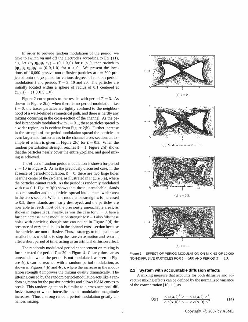
The effect of random period modulation is shown for periT = 10 in Figure 3. As in the previously discussed case, inabsence of period-modulation,ε = 0, there are two large holenear the center of theyz-plane, as illustrated in Figure 3(a), whethe particles cannot reach. As the period is randomly modultedwith ε = 0.1, Figure 3(b) shows that these unreachable islabecome smaller and the particles spread into a much widerain the cross-section. When the modulation strengthε is increasedto 0.5, these islands are nearly destroyed, and the particles arenow able to reach most of the previously unreachable areasshown in Figure 3(c). Finally, as was the case forT = 3, here afurther increase in the modulation strength toε = 1 also fills theseholes with particles; though one can notice in Figure 3(d)epresence of very small holes in the channel cross-section becausethe particles are non-diffusive. Thus, a strategy to fill up all thesesmaller holes would be to stop the transverse motion and restart itafter a short period of time, acting as an artificial diffusion effect.

The randomly modulated period enhancement on mixinfurther tested for periodT = 20 in Figure 4. Clearly those areaunreachable when the period is not modulated, as seen inure 4(a), can be reached with a random period-modulationshown in Figures 4(b) and 4(c), where the increase in the mo-lation strengthε improves the mixing quality dramatically. Thjittering caused by the random period-modulation acts likea ran-dom agitation for the passive particles and allows KAM curves tobreak. This random agitation is similar to a cross-sectional dif-fusive transport which intensifies as the modulation magnitudeincreases. Thus a strong random period-modulation greatlyen-hances mixing.

e11)

-

d-ea

i.or-a

o

odthesreandsare

s, a

th

g issFig-, asdu

e

z

y

0 0.5 1 1.5 20

0.5

1

(a) ε = 0.

z

y

0 0.5 1 1.5 20

0.5

1

(b) Modulation valueε = 0.1.

z

y

0 0.5 1 1.5 20

0.5

1

(c) ε = 0.5.

z

y

0 0.5 1 1.5 20

0.5

1

(d) ε = 1.


NON-DIFFUSIVE PARTICLES FOR t = 500AND PERIOD T = 10.

2.2 System with accountable diffusion effectsA mixing measure that accounts for both diffusive and ad-

vective mixing effects can be defined by the normalized varianceof the concentration [10,11], as

Θ(t) =< c(x,t)2 > − < c(x,t) >2

2 2 , (14)
< c(x,0) > − < c(x,0) >
5 Copyright c© 2007 by ASME

l

z

y

0 0.5 1 1.5 20

0.5

1

(a) ε = 0.

z

y

0 0.5 1 1.5 20

0.5

1

(b) Modulation valueε = 0.1.

z

y

0 0.5 1 1.5 20

0.5

1

(c) ε = 1.


NON-DIFFUSIVE PARTICLES FOR t = 500AND PERIOD T = 20.

where the spatial average<> in Eq. (14) is carried out over theentire domain. The quality of mixingΘ, is a positive function oftimet, and its value approaches zero if the final state is uniformmixed. The slope of theΘ curve is a measure of the rate at whichparticles in the solution mix; a steep drop inΘ is indicative of afast mixing rate. To study the interplay between random period-modulation and molecular diffusion, we turnoff the primary flowand the diffusion along the channel, and analyze the transverse-electric-driven flow in the two-dimensional cavity by meansofthe varianceΘ.

For purposes of studying the time-scale to obtain a sufficiently homogeneous product, a circular blob of reagent of ini-tial concentrationco =< c(y,z,0) >= 1, and radius 0.1, is cen-tered at(y,z) = (0.5,1). The quality of mixingΘ is then com-puted for Peclet numbers 104 and 105 by solving the convection-diffusion equation (12) for two different periods,T = 10 andT = 20 (St= 0.6 andSt= 0.3). The Reynolds number is 0.04.

6

y

-

The varianceΘ is plotted as a function of timet for three cases:(a) pure diffusion (no fluid motion), (b) electro-osmotic motionand no period modulation,ε = 0; and (c) electro-osmotic mo-tion and strong period modulation,ε = 1. In Figures 5 and 6 thePeclet numberPe is set to 105 so that diffusive effects are weakwhen fluid motion is present. From the figures it can be seen thatfor pure diffusion, the value ofΘ decays monotonically. Whenelectro-osmotic motion is present, after the initial 10 time-unitsthe value ofΘ drops much faster than that of the pure diffusioncase (keep in mind that a lower value ofΘ indicates a more ho-mogeneous state). The quality of mixing in Figure 5 shows theeffect of the stochastic period modulation protocol. The periodmodulation effect manifests itself whent &100 with an acceler-ated drop in the variance when compared to the purely diffusivesolution and to the stirring solution without such random pertur-bation. On the other hand, from Figure 6 it can be seen that,

t

Θ

10-1 100 101 102 10310-3

10-2

10-1

100

Figure 5. MIXING QUALITY Θ VS. TIME t , FOR T = 10; Re= 0.04and Pe= 105. -4- PURE DIFFUSION; -◦- NO PERIOD MODULATION;

-♦- PERIOD MODULATION WITH ε = 1.

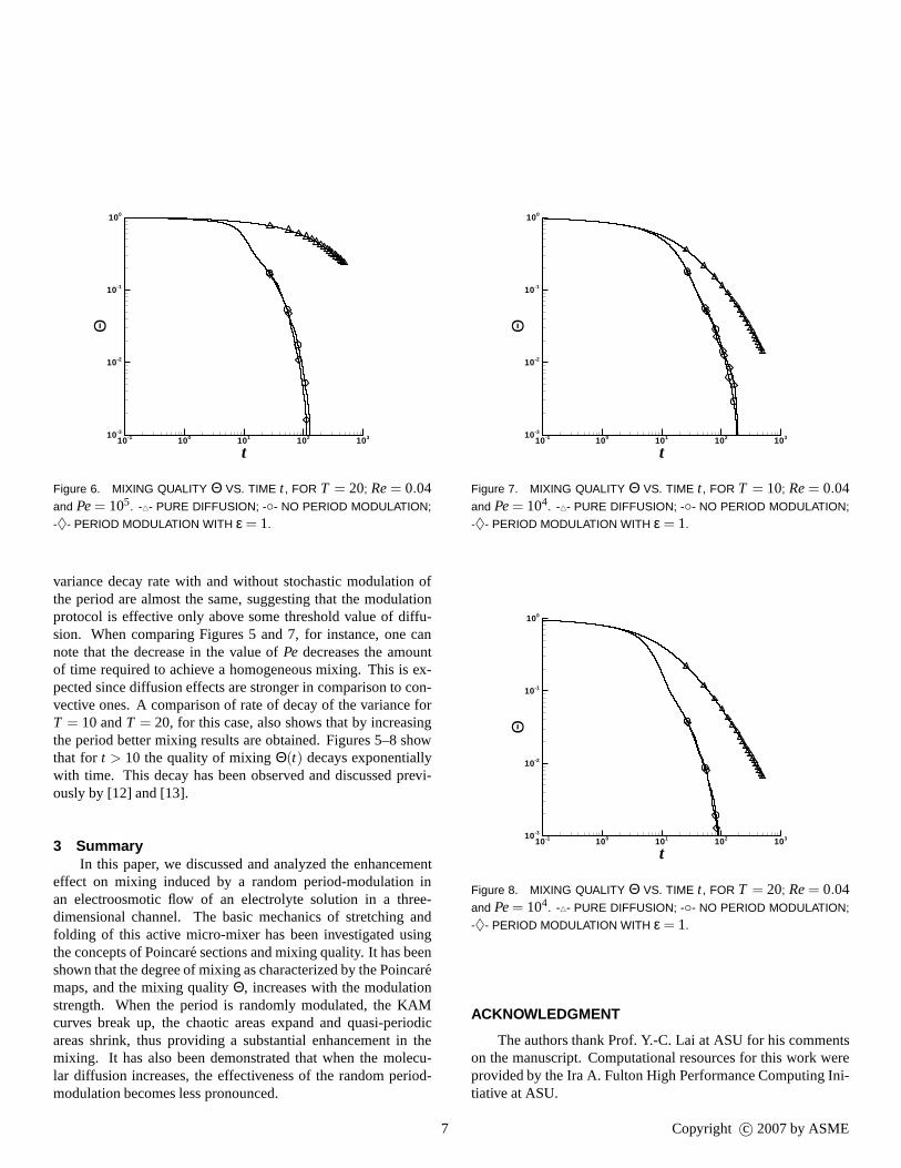
when the period is increased toT = 20, the randomization proto-col is much less effective. The stochastic solution is essentiallyequivalent to the stirring one withε = 0, although both solutionsbeat the purely diffusive case. Since the shear in islands doesenhance mixing over pure diffusion, it is possible that the size ofthe islands in the present case are small enough so that the effectof breaking them has little impact on the quality of mixing. Alsonote that the increase of the periodT, acts as an artificial diffu-sivity for the fluid flow, and decreases the time needed to achievea fairly homogeneous mixing.

In Figures 7 and 8 the Peclet numberPe is set to 104 so thatdiffusive effects are stronger than the case analyzed above. The


t

Θ

10-1 100 101 102 10310-3

10-2

10-1

100



variance decay rate with and without stochastic modulationofthe period are almost the same, suggesting that the modulaonprotocol is effective only above some threshold value of diffu-sion. When comparing Figures 5 and 7, for instance, one cnote that the decrease in the value ofPe decreases the amountof time required to achieve a homogeneous mixing. This is epected since diffusion effects are stronger in comparison to con-vective ones. A comparison of rate of decay of the variance frT = 10 andT = 20, for this case, also shows that by increasinthe period better mixing results are obtained. Figures 5–8 showthat for t > 10 the quality of mixingΘ(t) decays exponentiallywith time. This decay has been observed and discussed preously by [12] and [13].

3 SummaryIn this paper, we discussed and analyzed the enhancem

effect on mixing induced by a random period-modulation ian electroosmotic flow of an electrolyte solution in a threedimensional channel. The basic mechanics of stretching afolding of this active micro-mixer has been investigated usingthe concepts of Poincare sections and mixing quality. It has beenshown that the degree of mixing as characterized by the Poincaremaps, and the mixing qualityΘ, increases with the modulationstrength. When the period is randomly modulated, the KAMcurves break up, the chaotic areas expand and quasi-periocareas shrink, thus providing a substantial enhancement inhemixing. It has also been demonstrated that when the moleclar diffusion increases, the effectiveness of the random period-modulation becomes less pronounced.

7

ti

an

x-

og

vi-

entn-nd

ditu-

t

Θ

10-1 100 101 102 10310-3

10-2

10-1

100



t

Θ

10-1 100 101 102 10310-3

10-2

10-1

100



ACKNOWLEDGMENT

The authors thank Prof. Y.-C. Lai at ASU for his commentson the manuscript. Computational resources for this work wereprovided by the Ira A. Fulton High Performance Computing Ini-tiative at ASU.


REFERENCES[1] Willey, M. J., and West, A. C., 2006. “A microfluidic

device to measure electrode response to changes in elec-trolyte composition”.Electrochemical and Solid State Let-ters,9(7), pp. E17–E21.

[2] Chen, X., Cui, D. F., Liu, C. C., Li, H., and Chen, J., 2007.“Continuous flow microfluidic device for cell separation,cell lysis and DNA purification”.Analytica Chimica Acta,584(2), pp. 237–243.

[3] Pacheco, J. R., Chen, K. P., and Hayes, M. A., 2006. “Ef-ficient and rapid mixing in a slip-driven three-dimensionalflow in a rectangular channel”.Fluid Dyn. Res.,38(8),pp. 503–521.

[4] Pacheco, J. R., Chen, K. P., pacheco Vega, A., Chen, B., andHayes, M. A., 2007. Chaotic Mixing in an Electro-OsmoticFlow in a Rectangular Channel. (preprint).

[5] Leonard, B. P., 1979. “A stable and accurate convectivemodelling procedure based on quadratic upstream interpo-lation”. Comput. Methods Appl. Mech. Engng.,19, pp. 59–98.

[6] Zang, Y., Street, R. L., and Koseff, J. R., 1994. “A non-staggered grid, fractional step method for time dependentincompressible Navier-Stokes equations in curvilinear co-ordinates”.J. Comput. Phys.,114, pp. 18–33.

[7] Pacheco, J. R., and Peck, R. E., 2000. “Non-staggered gridboundary-fitted coordinate method for free surface flows”.Numer. Heat Transfer, Part B,37, pp. 267–291.

[8] Pacheco, J. R., 2001. “The solution of viscous incompress-ible jet flows using non-staggered boundary fitted coordi-nate methods”.Int. J. Numer. Meth. Fluids,35, pp. 71–91.

[9] Ottino, J. M., 1989.The kinematics of mixing: stretching,chaos and transport. Cambridge University Press., Cam-bridge, U.K.

[10] Batchelor, G. K., 1959. “Small-scale variation of convectedquantities like temperature in turbulent fluid. Part 1. Gen-eral discussion and the case of small conductivity”.J. FluidMech.,5, pp. 113–133.

[11] Danckwerts, P. V., 1952. “The definition and measurementof some characteristics of mixtures”.Appl. Sci. Res.,3,pp. 279–296.

[12] Pierrehumbert, R. T., 1994. “Tracer microstructure inthelarge-eddy dominated regime”.Chaos Solitons and Frac-tals,4, pp. 1091–1110.

[13] Antonsen Jr., T. M., Fan, Z., Ott, E., and Garcia-Lopez,E., 1996. “The role of chaotic orbits in the determina-tion of power spectra of passive scalars”.Phys. Fluids,8,pp. 3094–3104.

8 Copyright c© 2007 by ASME

Enhancement of Chaotic Mixing in Electroosmotic Flows …rpacheco/MIXING/IMECE2007-42707.pdf ·...

Documents

Transcript of Enhancement of Chaotic Mixing in Electroosmotic Flows …rpacheco/MIXING/IMECE2007-42707.pdf ·...