Enhanced Multicarrier Techniques for Professional Ad … · Enhanced Multicarrier Techniques for...
68
ICT 318362 EMPhAtiC Date: 17/06/2014 ICT-EMPhAtiC Deliverable D5.2 1/68 E nhanced M ulticarrier Techniques for P rofessional A d-Hoc and Cell-Based C ommunications (EMPhAtiC) Document Number D5.2 Novel algorithms description and performance evaluation for RRM in cell-based and ad-hoc PMR networks Contractual date of delivery to the CEC: 31/05/2014 Actual date of delivery to the CEC: 17/06/2014 Project Number and Acronym: 318362 EMPhAtiC Editor: Dimitris Tsolkas (CTI) Authors: Dimitris Tsolkas (CTI), Antonio Cipriano (TCS), Luxmiram Vijayandran (TCS), Mylene Pischella (CNAM), Juwendo Denis (CNAM) Participants: CTI,CNAM,TCS,CTTC Workpackage: WP5 Security: Public (PU) Nature: Report Version: 1.0 Total Number of Pages: 68 Abstract: This report provides a thorough study of Radio Resource Management (RRM) algorithms applied on top of Filter Bank Multicarrier (FBMC) physical layer scheme, and proposes solutions for optimizing the RRM performance in PMR networks. Open issues on RRM for PMR communications are also discussed, while both synchronized and unsynchronized communication scenarios for cell-based and ad hoc network deployments are examined. A proportional fair-based scheduling scheme for prioritizing critical PMR traffic inside a cell is studied, while, different resource allocation algorithms are proposed, providing theoretical optimizations and simulation-based evaluation results on top of FBMC.
-
Upload
truongthien -
Category
Documents
-
view
230 -
download
0
Transcript of Enhanced Multicarrier Techniques for Professional Ad … · Enhanced Multicarrier Techniques for...
ICT 318362 EMPhAtiC Date: 17/06/2014
ICT-EMPhAtiC Deliverable D5.2 1/68
Enhanced Multicarrier Techniques for Professional Ad-Hoc and Cell-Based Communications
(EMPhAtiC)
Document Number D5.2
Novel algorithms description and performance evaluation for RRM in cell-based and ad-hoc PMR networks
Contractual date of delivery to the CEC: 31/05/2014
Actual date of delivery to the CEC: 17/06/2014
Project Number and Acronym: 318362 EMPhAtiC
Editor: Dimitris Tsolkas (CTI)
Authors: Dimitris Tsolkas (CTI), Antonio Cipriano (TCS), Luxmiram Vijayandran (TCS), Mylene Pischella (CNAM), Juwendo Denis (CNAM)
Participants: CTI,CNAM,TCS,CTTC Workpackage: WP5 Security: Public (PU) Nature: Report Version: 1.0 Total Number of Pages: 68
Abstract: This report provides a thorough study of Radio Resource Management (RRM) algorithms applied on top of Filter Bank Multicarrier (FBMC) physical layer scheme, and proposes solutions for optimizing the RRM performance in PMR networks. Open issues on RRM for PMR communications are also discussed, while both synchronized and unsynchronized communication scenarios for cell-based and ad hoc network deployments are examined. A proportional fair-based scheduling scheme for prioritizing critical PMR traffic inside a cell is studied, while, different resource allocation algorithms are proposed, providing theoretical optimizations and simulation-based evaluation results on top of FBMC.
ICT 318362 EMPhAtiC Date: 17/06/2014
ICT-EMPhAtiC Deliverable D5.2 2/68
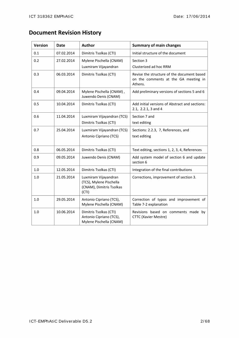
Document Revision History
Version Date Author Summary of main changes
0.1 07.02.2014 Dimitris Tsolkas (CTI) Initial structure of the document
0.2 27.02.2014 Mylene Pischella (CNAM) Luxmiram Vijayandran
Section 3 Clusterized ad hoc RRM
0.3 06.03.2014 Dimitris Tsolkas (CTI) Revise the structure of the document based on the comments at the GA meeting in Athens.
0.4 09.04.2014 Mylene Pischella (CNAM) , Juwendo Denis (CNAM)
Add preliminary versions of sections 5 and 6
0.5 10.04.2014 Dimitris Tsolkas (CTI) Add initial versions of Abstract and sections: 2.1, 2.2.1, 3 and 4
0.6 11.04.2014 Luxmiram Vijayandran (TCS) Dimitris Tsolkas (CTI)
Section 7 and text editing
0.7 25.04.2014 Luxmiram Vijayandran (TCS) Antonio Cipriano (TCS)
Sections: 2.2.3, 7, References, and text editing
0.8 06.05.2014 Dimitris Tsolkas (CTI) Text editing, sections 1, 2, 3, 4, References
0.9 09.05.2014 Juwendo Denis (CNAM) Add system model of section 6 and update section 6
1.0 12.05.2014 Dimitris Tsolkas (CTI) Integration of the final contributions
1.0 21.05.2014 Luxmiram Vijayandran (TCS), Mylene Pischella (CNAM), Dimitris Tsolkas (CTI)
Corrections, improvement of section 3.
1.0 29.05.2014 Antonio Cipriano (TCS), Mylene Pischella (CNAM)
Correction of typos and improvement of Table 7-2 explanation
1.0 10.06.2014 Dimitris Tsolkas (CTI) Antonio Cipriano (TCS), Mylene Pischella (CNAM)
Revisions based on comments made by CTTC (Xavier Mestre)
ICT 318362 EMPhAtiC Date: 17/06/2014
ICT-EMPhAtiC Deliverable D5.2 3/68
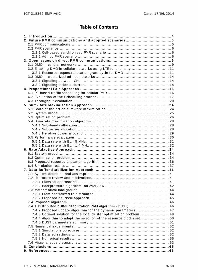
Table of Contents
1. Introduction ................................................................................................... 42. Future PMR communications and adopted scenarios ...................................... 5
2.1 PMR communications .................................................................................... 52.2 PMR scenarios .............................................................................................. 6
2.2.1 Cell-based synchronized PMR scenario ...................................................... 62.2.2 Ad hoc PMR scenario ............................................................................... 6
3. Open issues on direct PMR communications ................................................... 93.1 DMO in cellular networks ............................................................................... 93.2 Enabling DMO in cellular networks using LTE functionality ............................... 11
3.2.1 Resource request/allocation grant cycle for DMO ...................................... 113.3 DMO in clusterized ad-hoc networks ............................................................. 14
3.3.1 Signaling between CHs ......................................................................... 143.3.2 Signaling inside a cluster ....................................................................... 14
4. Proportional Fair Approach .......................................................................... 164.1 PF-based traffic scheduling for cellular PMR ................................................... 164.2 Evaluation of the Scheduling process ............................................................ 174.3 Throughput evaluation ................................................................................ 20
5. Sum-Rate Maximization Approach ................................................................ 245.1 State of the art on sum-rate maximization .................................................... 245.2 System model ............................................................................................ 255.3 Optimization problem .................................................................................. 265.4 Sum-rate maximization algorithm ................................................................. 28
5.4.1 Sub-bands allocation ............................................................................ 285.4.2 Subcarrier allocation ............................................................................. 285.4.3 Iterative power allocation ...................................................................... 29
5.5 Performance evaluation ............................................................................... 305.5.1 Data rate with Btot=5 MHz ..................................................................... 315.5.2 Data rate with Btot=1.4 MHz .................................................................. 32
6. Rate Adaptive Approach ............................................................................... 346.1 System model ............................................................................................ 346.2 Optimization problem .................................................................................. 346.3 Proposed resource allocation algorithm ......................................................... 366.4 Simulation results ....................................................................................... 37
7. Data Buffer Stabilization Approach .............................................................. 417.1 System definition and assumptions ............................................................... 417.2 Literature review and motivations ................................................................. 41
7.2.1 Classical approaches ............................................................................. 417.2.2 Backpressure algorithm, an overview ...................................................... 42
7.3 Mathematical background ............................................................................ 447.3.1 From centralized to distributed ............................................................... 447.3.2 Proposed heuristic approach .................................................................. 45
7.4 Proposed algorithm ..................................................................................... 467.4.1 Distributed bUffer Stabilization RRM algorithm (DUST) ................................. 46
7.4.2 Proposed update algorithm for the dynamic parameters ............................ 477.4.3 Optimal solution for the local cluster optimization problem ........................ 497.4.4 Algorithm to adapt the selection of the resource blocks set ........................ 507.4.5 DUST parameters summary ................................................................... 51
7.5 Numerical experiments ............................................................................... 527.5.1 Simulations objectives .......................................................................... 527.5.2 Detailed settings .................................................................................. 527.5.3 Numerical results ................................................................................. 55
7.6 Miscellaneous discussions ............................................................................ 638. Conclusions .................................................................................................. 659. References ................................................................................................... 66
ICT 318362 EMPhAtiC Date: 17/06/2014
ICT-EMPhAtiC Deliverable D5.2 4/68
1. Introduction This report describes the work carried out within T5.2 “Cell-based filter bank-based multicarrier (FBMC) for Radio resource management (RRM)” and T5.3 “Ad hoc FBMC for RRM” of the EMPhAtiC (Enhanced Multicarrier Techniques for Professional Ad-Hoc and Cell-Based Communications) project. The focus is on studying RRM algorithms applied on top of FBMC and investigating solutions for optimizing RRM performance in cell-based and ad hoc Professional Mobile Radio (PMR) networks.
Capitalizing on recent EMPhAtiC results (some of them provided in D5.1), we quantify the FBMC performance in RRM level under different network deployments and synchronization guarantees. Adopting the PMR terminology, user devices are referred to as Hand Helds (HHs) or Mobile Station (MSs). They establish direct links or links to a centric node, which is referred to as base station (BS) or cluster head (CH), for static and dynamic network deployment, respectively. In all the cases, the central node is responsible for RRM procedures such as the resource allocation and the traffic scheduling.
More specifically, in this report a comprehensive study on current advances on commercial cellular and dedicated public safety networks is provided, discussing the expected convergence of the standardization efforts in these two network types. Moving one step further and recognizing the importance of the incorporation of direct communications for public safety in future cellular networks, a complete resource request/grant cycle for DMO (Direct Mode Operation) in cellular systems is described, using as a benchmark system the Long Term Evolution (LTE). Sequentially, a traffic scheduling algorithm for QoS provision and prioritization of the critical PMR traffic inside a cell is proposed, borrowing the principles of the Proportional Fair (PF) scheduling. Finally, a series of different resource allocation schemes for PMR, each one of them applicable to different crisis scenario and network deployment, are proposed and optimized, while their performances on top of FBMC are quantified.
One of the most important outcomes of this report is the quantification of the FBMC superiority against CP-based approaches such as the OFDM, from the RRM point of view. Key parameter for this quantification is the adopted scenario and especially the available synchronization and coordination level. As resulted in this report, in the centrally controlled networks the absence of the CP for the FBMC case provides more resources for data transmission, while under loose synchronization in multi-user environments FBMC provides reduced adjacent channel interference and consequently higher bit rates.

ICT 318362 EMPhAtiC Date: 17/06/2014
ICT-EMPhAtiC Deliverable D5.2 5/68
2. Future PMR communications and adopted scenarios
2.1 PMR communications Currently, there are two separate technology communities for providing terrestrial wide-area wireless communications; the commercial cellular networks, based on standards such as the Long Term Evolution (LTE), and the dedicated public safety networks, based on standards such as the TETRA and P25. On the one hand, commercial cellular networks have been driven by the needs of consumer and business users, while their exceptional success has led to excellent economies of scale and constant rapid innovation. Public safety networks, on the other hand, provide communications for services like police, fire and ambulance. The focus here is on developing systems that are highly robust and can address the specific communication needs of emergency services. To this end, these systems have adopted a set of features that were not previously supported in commercial cellular systems. From the market’s perspective, the public safety users are an important community both economically and socially, but the market for systems based on public safety standards is much smaller.
Taking all the above into account, the convergence (establishment of common standards) of commercial cellular and public safety systems is expected to provide advantages to both of the communities. The public safety community will get access to the economic and technical advantages generated by the scale of commercial cellular networks, while the commercial cellular community will get the opportunity to address parts of the public safety market as well as gaining enhancements to their systems that have interesting applications to consumers and businesses.
Enhanced TETRA standards already support medium speed data (hundreds of kilobits per second) but it is recognized that new technology is needed to add true mobile broadband capabilities. In parallel, a lot of effort is currently devoted by 3GPP towards incorporating PMR communications in future LTE releases (especially Rel. 12). The main objective is to preserve the considerable strengths of LTE, while also adding features needed for public safety. A further goal is to maximise the technical commonality between commercial and public safety aspects to provide the best and most cost-effective solution for both communities. The main research areas towards addressing public safety applications in LTE are [1]: i) Proximity services (ProSe) that discover mobiles in physical proximity and enable optimized communications between them, and ii) group call system enablers (GCSE_LTE) that support the fundamental requirement for efficient and dynamic group communications operations such as one-to-many calling and dispatcher working. In both areas there are many challenges for the physical and higher layers, including: operation under loose synchronization, support of very low set-up time, guarantee of highly reliable and robust connections etc. Under these challenges, FBMC-based schemes are potentially the most suitable candidates for PMR communication. To provide a clear comparison of FBMC with its opponents from the RRM point of view, a variety of PMR scenarios and network deployments has been adopted as described in the following section.

ICT 318362 EMPhAtiC Date: 17/06/2014
ICT-EMPhAtiC Deliverable D5.2 6/68
2.2 PMR scenarios
2.2.1 Cell-based synchronized PMR scenario This scenario refers to the cell-based PMR communications, where in each cell, time and frequency synchronized cellular (and potentially direct - DMO) transmissions take place under the control of a base station (BS). It is assumed that network dimensioning/planning procedures have taken place, while the BSs are inter-connected through a backbone infrastructure. The Hand Helds (HHs) and the Mobile Stations (MS) are randomly deployed in each cell, while the transmissions of a dynamic set of HHs/MSs may be critical referring to communications for PPDR.
This scenario may model situations such as a car accident, train crash, traffic jam, etc., where coordination among police officers/firemen is needed at a specific area inside a cell (Fig. 2-1). Practically, specific set of HHs/MSs requires scheduling priority, since their transmissions carry vital information. The BS must serve the critical traffic with priority and guarantee the QoS (Quality of Service) requirements of the non-critical traffic as well.
Figure 2-1: illustration of the cell-based PMR scenario
2.2.2 Ad hoc PMR scenario
In this ad-hoc scenario, we investigate two different applications:
PMR with external services: an ad-hoc network deployed in a random area where a BS is in charge of all RRM and enables communication to the outside-world. Imagine for example a town after an earth-quake where all communication backbone infrastructures are unusable. A unique BS-like element needs to be deployed to handle the local communications as well as the outside-connection.

ICT 318362 EMPhAtiC Date: 17/06/2014
ICT-EMPhAtiC Deliverable D5.2 7/68
When multiple BS are deployed no inter-connection/ coordination among them is available.
PMR with locally-limited communications: the communication is restricted within a local area. A node is elected as Cluster Head (CH) and will be in charge of the RRM, but does not relay any data. If the area is large, multiple clusters will be formed (i.e., through discovery), each one with its own elected CH, while a broadcast control channel will be used for inter-connection between CHs. Imagine for example a localized area where a fire is to be stopped. The firemen and the policemen are randomly deployed, without any deployed BS, and need for a short period of time to communicate (i.e., Point-to-Point or Point-to-Multicast).
The two applications are described in more details hereafter.
2.2.2.1 PMR with external services
In this scenario, several BSs are randomly located in space. The MSs also follow a non-uniform spatial distribution. Poisson Point Process or Binomial Point Process [2] may for instance model such distributions. In this scenario, there may be either non-covered areas, or on the contrary areas with high levels of interference. Additionally, the BSs are completely independent of each other and there is no backbone infrastructure to inter-connect them. Each active HH/MS is connected to its closest BS.
We assume that the BSs transmissions are unsynchronized in this crisis situation and all BSs have different clocks. On the other hand, within one cell (i.e., one BS’s coverage area), all transmissions between the HHs/MSs and the BS are synchronized, in uplink as well as in downlink.
This scenario models a crisis situation, where there is no infrastructure-based PMR network, including events such as: a tsunami, earthquake or flooding destroying any prior network infrastructure in a dense area, such as a city. It may also be used by policemen who need to deploy their PMR network into strategic positions rapidly enough and at low cost, where PMR networks are not yet existing or have been destroyed by natural disasters or bombing. The BSs may also be moving, following the firemen or policemen positions. To this end, an ad hoc PMR network must be spread very rapidly, without any prior planning study. The ad hoc PMR BSs are supposed of low complexity and are consequently not equipped with any direct wired or wireless interface allowing them to exchange with one another. The HHs/MS may use several applications required for PMR activities, such as voice, video-conferencing, or FTP. All data sent from a HH/MS to its serving BS is then transferred to a distant controlling server. The controlling server is not used to manage the radio access network, but only to manage the firemen or policemen activities.
2.2.2.2 PMR with locally-limited communications
In this scenario multiple nodes are deployed on a given area, discover their surrounding, and group themselves into different clusters with one elected cluster head (CH). The clustering decision can depend on different criteria e.g., operational constraints, channel quality, multi-hops constraints, but is not investigated here. Each elected CH of a given cluster is responsible for the RRM of all the associated internal links, only. The selection of the ‘best’ CH is related to its relative location and channel quality with all other nodes of the same cluster. It is therefore likely that the CH election can change in time (although a trade-off needs to be achieved between using the node having the best links quality with others and

ICT 318362 EMPhAtiC Date: 17/06/2014
ICT-EMPhAtiC Deliverable D5.2 8/68
the selection stability to avoid too much signaling for changing CH). It is assumed that only one link in a given cluster can use a given spectrum resource unit, referred to as resource block (RB).
The elected CH (following neighbors discovery and CH election protocol) is in charge of RRM allocation for all associated HH, but different from a BS do not relay any data. Control information is assumed from the CH to the HHs (i.e., RRM allocation) as well as from the HHs to the CH (i.e., feedback information such as channel quality). It is assumed that perfect frequency and time synchronization is available inside each cluster controlled by the CH. In terms of data transmission different clusters are unsynchronized with different clocks. However, it is assumed that a broadcast control channel (with small capacity) is available for each CH to inform other surrounding CHs, but collisions may appear when more than one CH transmits at the same time. To this end, a simple solution is the use of a unique pilot signal, known by all clusters, which can be detected before analyzing the content. Note that if inter-communication is required, some nodes need to play the role of gateway, but this issue is not investigated in this deliverable.

ICT 318362 EMPhAtiC Date: 17/06/2014
ICT-EMPhAtiC Deliverable D5.2 9/68
3. Open issues on direct PMR communications
3.1 DMO in cellular networks Referring to the scenario described in section 2.2.1 (cell-based synchronized PMR), one of the main characteristics of the PMR communications is that HHs/MSs can communicate directly without the intermediate transmissions to the BS. In future broadband PMR communications (as described in section 2.1), conventional PMR and commercial cellular networks will converge, and thus, the DMO must be enabled in the framework of the mobile cellular systems. Adopting the LTE system as a case study, already standardized signaling could support the cellular broadband PMR communications, by using separated bands for PMR transmissions. However, major challenges must be addressed before LTE incorporates the DMO. These challenges include issues such as the synchronization of the peers, the device discovery, and the resource allocation for DMO [3].
The problem of synchronizing DMO transmissions is very challenging because the transmitter and the receiver inside the cell can be any HH, breaking the rule in cellular communications where the BS is the unique node that transmits during the DL and receives during the UL. Even though two HHs are in coverage and synchronized to their corresponding BSs, the synchronization between them for DMO communication is not guaranteed since: i) they may be associated with different BSs that are not synchronized, and ii) they may have different distances to the BS and different timing advance adjustments may be applied. The problem is much more difficult for out of coverage HHs, as in the scenario described in section 2.2.2.2. In this case, there is no BS to transmit synchronization signals and hence the design of synchronization signals for DMO is needed. To this end, cluster head (CH) nodes can be used to transmit synchronization reference signals. A CH may be an authorized HH that transmits the BS-like synchronization reference signals in its communication range. The FBMC PHY is probably a good candidate for DMO since the performance of the FBMC in unsynchronized environments is quite better than its opponents.
Synchronization
A major challenge prior the introduction of DMO operation in cellular networks is the device discovery problem, i.e., the problem of meeting the communication peers in time, frequency and space. The device discovery procedure may involve the core network or not. In the latter case, a HH would search for nearby HHs autonomously, while the discovery scheme is more flexible and scalable, since it operates under local-level requirements and the complexity is transported at the end-users. It is also a suitable solution in case of out-of-coverage DMO. Practically, HHs participate in a device discovery process where periodically they transmit/receive discovery signals. These signals can include broadcast information, in which a HH announces its presence or information regarding specific discoverable HHs. Another open issue in device discovery is the design of the discovery signal, i.e., the decision on what kind of information should be carried by the discovery signals. For unsynchronized discovery transmissions, a potential approach is to embed limited discovery information into reference signals. However, in the case of synchronized discovery transmissions rich discovery information, such as the discoveree’s identity or
Device discovery
ICT 318362 EMPhAtiC Date: 17/06/2014
ICT-EMPhAtiC Deliverable D5.2 10/68
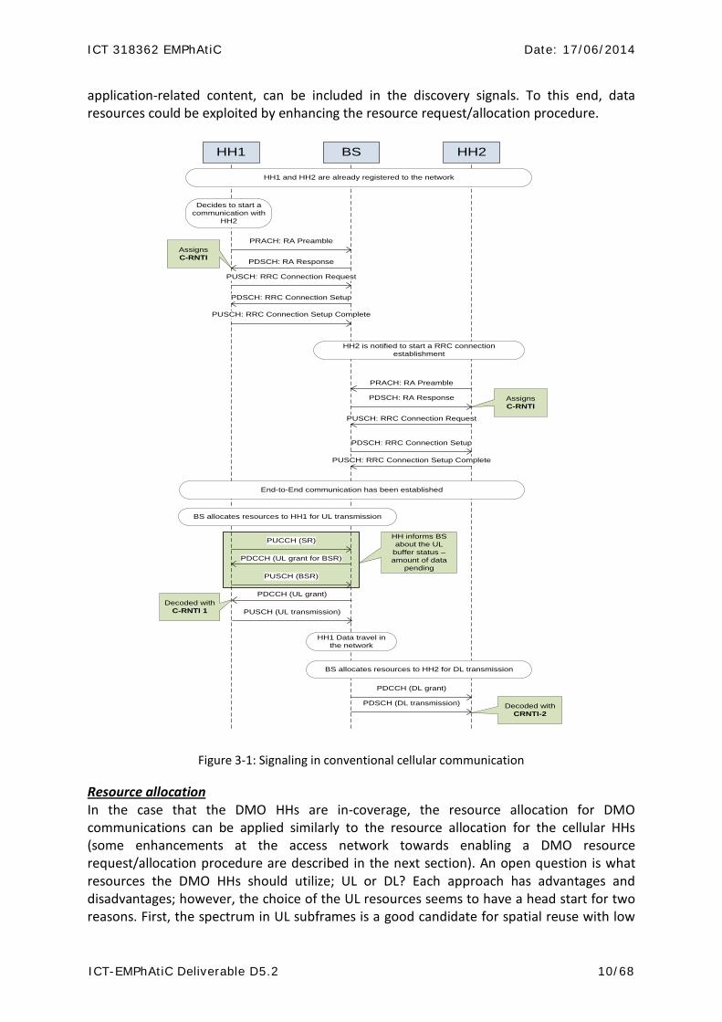
application-related content, can be included in the discovery signals. To this end, data resources could be exploited by enhancing the resource request/allocation procedure.
Figure 3-1: Signaling in conventional cellular communication
In the case that the DMO HHs are in-coverage, the resource allocation for DMO communications can be applied similarly to the resource allocation for the cellular HHs (some enhancements at the access network towards enabling a DMO resource request/allocation procedure are described in the next section). An open question is what resources the DMO HHs should utilize; UL or DL? Each approach has advantages and disadvantages; however, the choice of the UL resources seems to have a head start for two reasons. First, the spectrum in UL subframes is a good candidate for spatial reuse with low
Resource allocation
HH1 BS HH2
PRACH: RA Preamble
PUSCH: RRC Connection Request
PDSCH: RA Response
PDSCH: RRC Connection Setup
PUCCH (SR)
PUSCH (BSR)
PDCCH (UL grant for BSR)
Assigns C-RNTI
PUSCH: RRC Connection Setup Complete
PDCCH (DL grant)
HH1 and HH2 are already registered to the network
Decides to start a communication with
HH2
HH2 is notified to start a RRC connection establishment
PDSCH (DL transmission)
PUSCH (UL transmission)Decoded with
C-RNTI 1
PDCCH (UL grant)
BS allocates resources to HH1 for UL transmission
PRACH: RA Preamble
PUSCH: RRC Connection Request
PDSCH: RA Response
PDSCH: RRC Connection Setup
Assigns C-RNTI
PUSCH: RRC Connection Setup Complete
Decoded with CRNTI-2
HH1 Data travel in the network
BS allocates resources to HH2 for DL transmission
End-to-End communication has been established
HH informs BS about the UL
buffer status – amount of data
pending

ICT 318362 EMPhAtiC Date: 17/06/2014
ICT-EMPhAtiC Deliverable D5.2 11/68
impact to cellular communications, since during the UL the only cellular interfered nodes are the immobile BSs. Secondly, the UL subframes are often less utilized than the DL ones, making room for additional transmissions.
3.2 Enabling DMO in cellular networks using LTE functionality In the case of the cellular communication mode, the conventional LTE procedure for request/allocation grant can be adopted, whatever is the physical layer (OFDM or FBMC). Fig. 3-1 illustrates this procedure, while a detailed description can be found in [4]. Referring to transmissions from and to BSs, there are two basic categories of communication subframes, for downlink (DL) and uplink (UL) transmission, respectively. The spectrum assignment for DL and UL transmissions is a BS responsibility, and thus, each BS uses MAC layer identities called Cell Radio Network Temporary Identifiers (C-RNTIs) to uniquely identify its serving HHs [4]. When a HH requests for resources, after a random access procedure, messages for establishing a RRC connection are exchanged between BS and HH (the HH from idle mode transit to connected mode). During this procedure, a unique C-RNTI is assigned by the BS to the requested HH. Note that the C-RNTIs are very important for the radio resource allocation procedure, since the coding/decoding of the physical downlink control channel (PDCCH) that includes the resource allocation grant is based on the C-RNTIs. Practically, each HH uses its C-RNTI to decode the individual resource allocation message transmitted to it by the BS, and, consequently, to identify the spectrum portion that it will use for reception (DL) or transmission (UL).
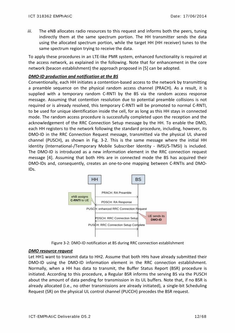
3.2.1 Resource request/allocation grant cycle for DMO Radio resource management is an open challenge for the enabling of ProSe in LTE. One of the directions in the standardization field requires a dynamic spectrum portion to be dedicated for direct communications under a resource request/allocation procedure. Differing from the conventional resource allocation procedure, in the resource allocation for DMO the BS must inform both the transmitter and receiver about the allocation grant, tuning them to the same allocated resources. Although the transmitter’s C-RNTI is known at the BS (it is included in the spectrum request message), the BS is not aware of transmitter’s C-RNTI. Thus, it cannot inform the potential receiver about the time and frequency that will be used. To overcome this problem, we propose the introduction of a new MAC layer identity, called DMO-ID. The main characteristic of this identity is that it is generated at each HH by using the application layer identity. In this way, when the application layer identity of a target HH is known at a HH that wants to announce its expression code, the target DMO-ID can be precisely produced. The serving BS, having a mapping between standardized identifiers (C-RNTIs) and DMO-IDs, uses the former ones as in the cellular communications in order to inform both peers about the resource allocation grant. In the following, we assume the case that individual DMO-IDs are used to simplify the description of the proposed scheme. The proposed scheme can be summarized in the following three steps:
i. Each HH produces its DMO-ID and transmits it to the serving BS during RRC connection establishment. Upon the reception of DMO-IDs, BS maps them to C-RNTIs.
ii. When the BS decides that data should be directly transmitted, the HH transmitter includes the DMO-ID of the target HH in a resource request message (as explained later in this section).
ICT 318362 EMPhAtiC Date: 17/06/2014
ICT-EMPhAtiC Deliverable D5.2 12/68
iii. The eNB allocates radio resources to this request and informs both the peers, tuning indirectly them at the same spectrum portion. The HH transmitter sends the data using the allocated spectrum portion, while the target HH (HH receiver) tunes to the same spectrum region trying to receive the data.
To apply these procedures in an LTE-like PMR system, enhanced functionality is required at the access network, as explained in the following. Note that for enhancement in the core network (beacon establishment) the approach proposed in [5] can be adopted.
Conventionally, each HH initiates a contention-based access to the network by transmitting a preamble sequence on the physical random access channel (PRACH). As a result, it is supplied with a temporary random C-RNTI by the BS via the random access response message. Assuming that contention resolution due to potential preamble collisions is not required or is already resolved, this temporary C-RNTI will be promoted to normal C-RNTI, to be used for unique identification inside the cell, for as long as this HH stays in connected mode. The random access procedure is successfully completed upon the reception and the acknowledgement of the RRC Connection Setup message by the HH. To enable the DMO, each HH registers to the network following the standard procedure, including, however, its DMO-ID in the RRC Connection Request message, transmitted via the physical UL shared channel (PUSCH), as shown in Fig. 3-2. This is the same message where the initial HH identity (International-/Temporary Mobile Subscriber Identity - IMSI/S-TMSI) is included. The DMO-ID is introduced as a new information element in the RRC connection request message [4]. Assuming that both HHs are in connected mode the BS has acquired their DMO-IDs and, consequently, creates an one-to-one mapping between C-RNTIs and DMO-IDs.
DMO-ID production and notification at the BS
Figure 3-2: DMO-ID notification at BS during RRC connection establishment
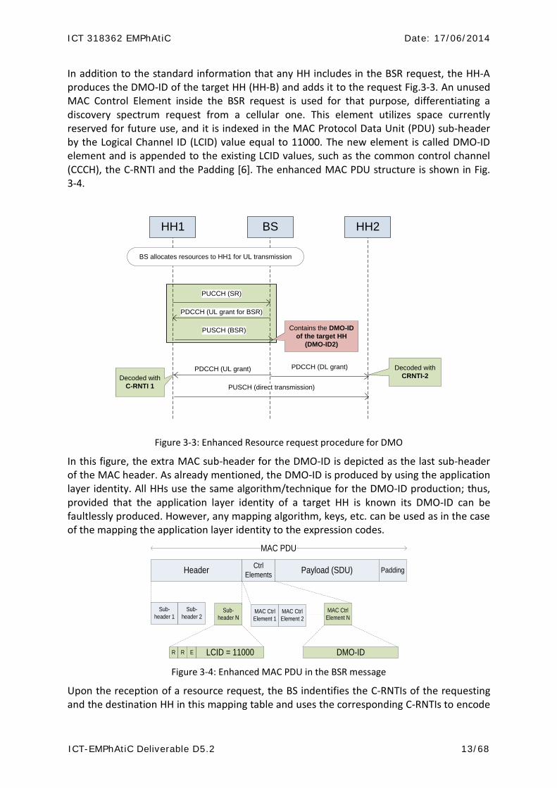
Let HH1 want to transmit data to HH2. Assume that both HHs have already submitted their DMO-ID using the DMO-ID information element in the RRC connection establishment. Normally, when a HH has data to transmit, the Buffer Status Report (BSR) procedure is initiated. According to this procedure, a Regular BSR informs the serving BS via the PUSCH about the amount of data pending for transmission in its UL buffers. Note that, if no BSR is already allocated (i.e., no other transmissions are already initiated), a single-bit Scheduling Request (SR) on the physical UL control channel (PUCCH) precedes the BSR request.
DMO resource request
PRACH: RA Preamble
PUSCH: enhanced RRC Connection Request
PDSCH: RA Response
PDSCH: RRC Connection SetupUE sends its
DMO-ID
eNB assigns C-RNTI to UE
PUSCH: RRC Connection Setup Complete
HH BS
ICT 318362 EMPhAtiC Date: 17/06/2014
ICT-EMPhAtiC Deliverable D5.2 13/68
In addition to the standard information that any HH includes in the BSR request, the HH-A
produces the DMO-ID of the target HH (HH-B) and adds it to the request Fig.3-3. An unused MAC Control Element inside the BSR request is used for that purpose, differentiating a discovery spectrum request from a cellular one. This element utilizes space currently reserved for future use, and it is indexed in the MAC Protocol Data Unit (PDU) sub-header by the Logical Channel ID (LCID) value equal to 11000. The new element is called DMO-ID element and is appended to the existing LCID values, such as the common control channel (CCCH), the C-RNTI and the Padding [6]. The enhanced MAC PDU structure is shown in Fig. 3-4.
Figure 3-3: Enhanced Resource request procedure for DMO
In this figure, the extra MAC sub-header for the DMO-ID is depicted as the last sub-header of the MAC header. As already mentioned, the DMO-ID is produced by using the application layer identity. All HHs use the same algorithm/technique for the DMO-ID production; thus, provided that the application layer identity of a target HH is known its DMO-ID can be faultlessly produced. However, any mapping algorithm, keys, etc. can be used as in the case of the mapping the application layer identity to the expression codes.
Header Payload (SDU)
Sub-header 1
Sub-header Ν
MAC Ctrl Element 1
MAC Ctrl Element N
R ER LCID = 11000 DMO-ID
MAC PDU
Ctrl Elements Padding
Sub-header 2
MAC Ctrl Element 2
Figure 3-4: Enhanced MAC PDU in the BSR message
Upon the reception of a resource request, the BS indentifies the C-RNTIs of the requesting and the destination HH in this mapping table and uses the corresponding C-RNTIs to encode
HH1 BS HH2
PUCCH (SR)
PUSCH (BSR)
PDCCH (UL grant for BSR)
PDCCH (DL grant)
PUSCH (direct transmission)Decoded with
C-RNTI 1
PDCCH (UL grant)
BS allocates resources to HH1 for UL transmission
Decoded with CRNTI-2
Contains the DMO-ID of the target HH
(DMO-ID2)
ICT 318362 EMPhAtiC Date: 17/06/2014
ICT-EMPhAtiC Deliverable D5.2 14/68
two allocation messages (allocation grant) for the HHs; one for the HH transmitter and one for the HH receiver (Fig. 3-3).
3.3 DMO in clusterized ad-hoc networks
3.3.1 Signaling between CHs
Referring to the scenario described in section 2.2.2.2, the control information can be either transmitted with another dedicated radio access technology (with higher coverage than the PMR system), or with the same radio access technology of the PMR system. In the latter case, one dedicated carrier, or part of the band, or a given TDMA sub-frame of the global frame (depending on the frame structure), can be allocated to that purpose. For this case, the coverage of the dedicated control channel will not be substantially different from the one of the PMR system, hence mechanisms must be found to extend this coverage. Several options are possible, ranging from the simple increase of power, to more complex relaying strategies combined with CSMA or with PHY / MAC techniques lowering the impact of collisions, for instance like multi-user detection. As an example, we can imagine the flooding of CH control messages with cooperative broadcast in which all the nodes of the network participate over the common channel. This topic is important and quite interesting also from a research perspective; however it has not been investigated here.
With asynchronous clusters, exchange of control information is still possible (e.g., through information mixed with reference pilots), yet will impose many constraints on the frame design or the choice of a MAC scheme working in asynchronous conditions (which is different from the MAC inside the cluster which is synchronous, thus increasing the complexity of supporting two different MAC mechanisms). The exact amount of signaling that can be exchanged depends on many parameters and it is not estimated here.
Note that the proposed algorithm for the clusterized ad-hoc networks, in Section 7 (i.e., the DUST algorithm), has not been tested with loss of signaling due to collisions. However, it is believed that the algorithm performance should not deteriorate much due to the simple characteristics of the information exchanged (i.e., cumulated data queue size of a cluster which can be a large value constantly varying in time).
3.3.2 Signaling inside a cluster For signaling inside a cluster two major approaches can be defined:
- If time division is possible: Signaling and Data happen in two time slots using the same resources. Looking at the MAC frame in time we would have 2 sub-frames: 1st a small time portion is used where only the CH transmits (i.e., broadcast the RRM decision to all HHs), and during the second sub-frame the HHs transmit data using the allocated resource. A guard time could be imposed between the 2 sub-frames to cope with resource changes.
- If time division is not possible: A dedicated band for the CH broadcast is required. Of course, HHs need to work in full duplex (i.e., receive/transmit data at the same time as they listen to the control broadcast on another band). Note that with current technologies it is not possible to use some sub-carriers for signaling reception while using the remaining sub-carriers for transmitting data within a given band. Thus, dedicated separate band is necessary.
ICT 318362 EMPhAtiC Date: 17/06/2014
ICT-EMPhAtiC Deliverable D5.2 15/68
Beyond the previous general discussion, another sensed assumption is that the PMR system uses a LTE (or LTE-like) protocol stack. This assumption is strengthened by the fact that LTE technology was chosen as the bases of next generation PRM services in the USA, and that 3GPP shows high activity in working groups related to extensions of LTE for covering typical PMR services. Notice also that the work in Section 4 uses this hypothesis of LTE-like protocol. Assuming an LTE-like protocol stack for the communications inside a cluster, the allocation information from the CH to the HHs can be embedded in the current Physical Downlink Control CHannel (PDCCH). Of course a new Downlink Control Information (DCI) format will be required, with slight modifications for signaling data transmissions between two HHs. As already mentioned, in the standardization field, such kind of issues will be tackled by the LTE Rel. 12 or the following.
Another issue concerning signaling is the information messages from the HH to the CH. We recall that these messages should convey information such as the link channel quality, as well as the local link data buffer size. LTE protocol already specified a Physical Uplink Control Channel (PUCCH) and also a mechanism for embedding long control information inside the Physical Uplink Shared Channel (PUSCH) which is the channel for data transmissions. Depending on the length of the information to be sent, rather than defining new formats of PUCCH, perhaps the most practical and easy way to include these messages are to send them inside the PUSCH. This proposal will in any case require modifications of the current LTE protocol, but those modifications are limited.
ICT 318362 EMPhAtiC Date: 17/06/2014
ICT-EMPhAtiC Deliverable D5.2 16/68
4. Proportional Fair Approach
4.1 PF-based traffic scheduling for cellular PMR In the infrastructure-based PMR networks the BSs have to provide priority to the critical traffic and guarantee the QoS requirements of both critical and non-critical communications as well. In this section, we adopt the cell-based, fully synchronized scenario described in section 2.2.1 and we provide a scheduling scheme based on the well known proportional fair (PF) algorithm.
The PF algorithm allocates the spectrum resources in each communication subframe (denoted here by s ) proportionally to the average data rate and the potential achievable data rate per user, using the following priority function:
( )( )( )
ii
i
r sP sR s
= (4.1)
where, i is the user index, ( )ir s is the potentially achieved data rate (based on channel conditions) if the resources are allocated to the candidate user, and ( )iR s is the average already provided data rate to the candidate user over a monitoring window of S subframes. In more detail, using Shannon limit: 𝑟𝑖(𝑠) = log2(1 + 𝑆𝑁𝑅𝑖(𝑠)):
1 11 ( ) ( ) If user i is scheduled( 1)
11 ( ) If user i is not scheduled
i i
i
i
R s r sS S
R sR s
S
− ⋅ + + =
− ⋅
(4.2)
There are three basic scheduling alternatives: Maximum Carrier to Interference (Max C/I) scheduling algorithm, Round Robin (RR) scheduling algorithm and conventional Proportional Fair (PF) scheduling algorithm. Max C/I chooses the users with the best channel gain, it results in the maximum system throughput. RR chooses users in turn, and gives users the equal scheduling probability without priority. RR scheduling algorithm results in the lowest throughput but the highest fairness. More specifically:
( )( )
( )( )
( )
ai
ii
r sP s
R s β= (4.3)
where, if 1a = and 1β = then we get the conventional PF scheduling, if 0a = and 1β = then we get the RR scheduling, and 1a = and 0β = if then we get the Max C/I scheduling.
In multicarrier systems the spectrum resources of a subframe can be allocated to multiple users. Let us denote by U the set of users that are allocated in a subframe and by iC the set of subcarriers allocated to user i in this subframe. Eq. 4.2 yields to Eq. 4.4,
( ) { } ,1 ( ) ( )( 1) i
i i U i cc C
i
S R s I r sR s
S
∈∈
− ⋅ ++ =
∑ (4.4)
where, {( )}I ∗ is 1 if ( )∗ is true, and 0 if ( )∗ is false.
ICT 318362 EMPhAtiC Date: 17/06/2014
ICT-EMPhAtiC Deliverable D5.2 17/68
The priority function depicted in Eq. 4.1, describes the generic PF algorithm assuming non- real-time traffic, and is the base on which various algorithms have been built. Here we adopt the exponential/proportional fair (EXP/PF) algorithm, where the priority function depends on the service type. More specifically, the priority function is:
( ) ( ) ( )exp for RT services( )1 ( )( )
( ) for NRT services( )
i i i
ii
i
i
v W s v W s r sR sv W sP s
r sR s
⋅ − ⋅ ⋅ + ⋅ = (4.5)
where, log( )ii
i
v δτ
= − , ( )iW s is the packet delay of user i at subframe s , iτ is the delay
threshold of user i’s packets (different for different services), iδ is the maximum acceptable
probability for packet delay to exceed the delay threshold of user i , and ( )v W s⋅ the mean value of the ( )i iv W s⋅ values in the system.
The idea is to change indirectly the behavior of the algorithm without losing its proportional fairness characteristic. Based on Eq. 4-5, the traffic with lower iδ values has no strict priority against the other traffic; however its requirements are guaranteed with very high probability. To this end, the BS chooses higher iδ values for the PMR traffic to guarantee indirectly higher reliability and more stable performance.
The priority function of the proposed scheme is as follows:
* *
*
( ) ( ) ( )exp for PMR RT services( )1 ( )
( ) ( ) ( )( ) exp for RT services( )1 ( )
( ) for NRT services( )
i i i
i
i i ii
i
i
i
v W s v W s r sR sv W s
v W s v W s r sP sR sv W s
r sR s
⋅ − ⋅ ⋅ + ⋅ ⋅ − ⋅= ⋅ + ⋅
(4.6)
where *
* log( )ii
i
v δτ
= − and *i iδ δ<
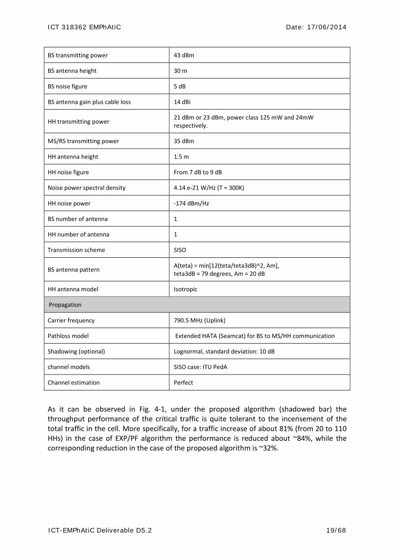
4.2 Evaluation of the scheduling process Towards comparing the proposed scheduling approach with the conventional EXP/PF scheme we monitor the UL throughput performance of a BS for 500 subframes assuming that a specific set of HHs that carries critical information. This set of HHs establishes critical VoIP connections, while the remaining traffic consists of non-critical VoIP and NRT flows. The used simulation parameters are depicted in Table 4-1.
In Fig. 4-1, we provide the performance of the proposed algorithm against the conventional EXP/PF algorithm when the number of non-critical flows in the network increases. This is a

ICT 318362 EMPhAtiC Date: 17/06/2014
ICT-EMPhAtiC Deliverable D5.2 18/68
common paradigm observed in crisis situations, where everybody tries to communicate and the traffic load increases rapidly.
Table 4-1: Simulation parameters
Parameter description Parameter value
Generic parameters
Number of different networks in the scenario
Single multi-cell network with coordinated and synchronized cells.
Scenarios Urban
Network All users and BSs are time and frequency synchronized, FDD
Spatial distribution of users Uniformly randomly distributed in the cell. Minimum distance between UE and BS >= 80 m.
Number of active users / cell 1 user, and 20 users
User mobility model Static
Traffic model Infinite Buffer, DL or/and UL continuous traffic.
Uplink scheduling EXP/PF and proposed PF schedulers
UL power control Yes
Frame structure
Bandwidth 1.4 MHz,
Subcarriers number 128 subcarriers, 72 useful
Frame length in time 10 ms OFDM, 8 ms FBMC (due to CP absence)
Subframe length (granularity in time) 1 ms (2 slots)
Subcarrier spacing 15 kHz
Number of symbols per subframe 15 (12 for data channel)
Allocation unity 1 Resource Block (RB)
RB spacing 180 kHz, 1 ms
Number of subcarriers per RB 12
Total number of resource elements per RB 12x15 = 180 (144 for data channels)
FBMC filter OFDM/OQAM PHYDYAS
Overlapping factor 4
Modulation and coding schemes MCSs based on LTE transport formats
Transmitter/Receiver
ICT 318362 EMPhAtiC Date: 17/06/2014
ICT-EMPhAtiC Deliverable D5.2 19/68
BS transmitting power 43 dBm
BS antenna height 30 m
BS noise figure 5 dB
BS antenna gain plus cable loss 14 dBi
HH transmitting power 21 dBm or 23 dBm, power class 125 mW and 24mW respectively.
MS/RS transmitting power 35 dBm
HH antenna height 1.5 m
HH noise figure From 7 dB to 9 dB
Noise power spectral density 4.14 e-21 W/Hz (T = 300K)
HH noise power -174 dBm/Hz
BS number of antenna 1
HH number of antenna 1
Transmission scheme SISO
BS antenna pattern A(teta) = min[12(teta/teta3dB)^2, Am], teta3dB = 79 degrees, Am = 20 dB
HH antenna model Isotropic
Propagation
Carrier frequency 790.5 MHz (Uplink)
Pathloss model Extended HATA (Seamcat) for BS to MS/HH communication
Shadowing (optional) Lognormal, standard deviation: 10 dB
channel models SISO case: ITU PedA
Channel estimation Perfect
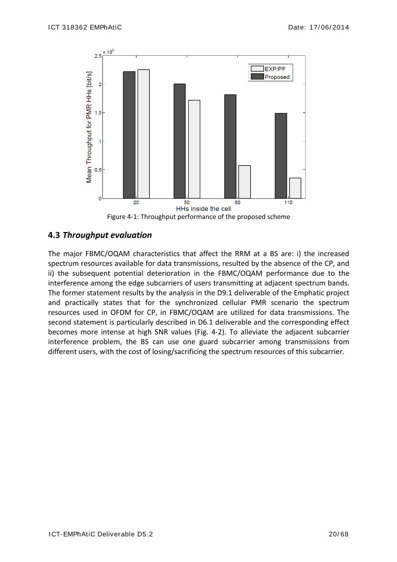
As it can be observed in Fig. 4-1, under the proposed algorithm (shadowed bar) the throughput performance of the critical traffic is quite tolerant to the incensement of the total traffic in the cell. More specifically, for a traffic increase of about 81% (from 20 to 110 HHs) in the case of EXP/PF algorithm the performance is reduced about ~84%, while the corresponding reduction in the case of the proposed algorithm is ~32%.
ICT 318362 EMPhAtiC Date: 17/06/2014
ICT-EMPhAtiC Deliverable D5.2 20/68
Figure 4-1: Throughput performance of the proposed scheme
4.3 Throughput evaluation
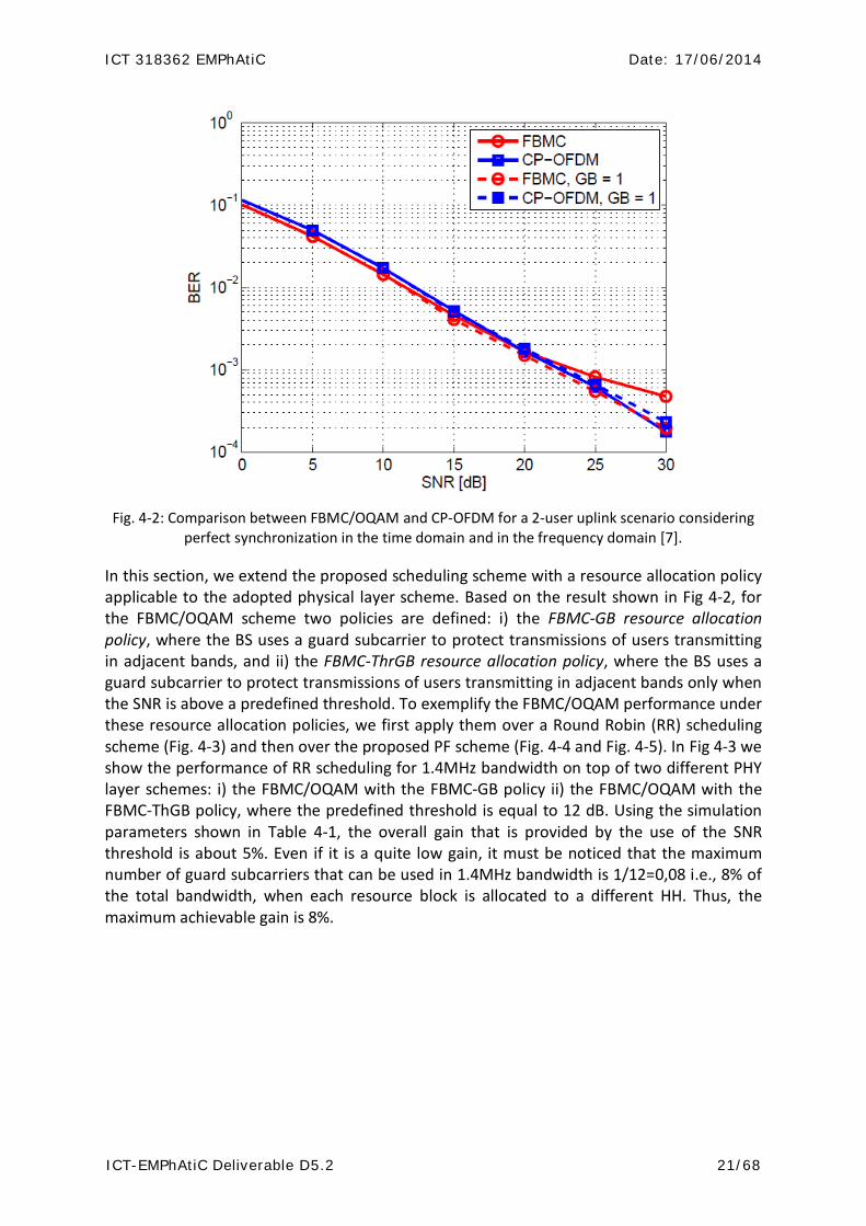
The major FBMC/OQAM characteristics that affect the RRM at a BS are: i) the increased spectrum resources available for data transmissions, resulted by the absence of the CP, and ii) the subsequent potential deterioration in the FBMC/OQAM performance due to the interference among the edge subcarriers of users transmitting at adjacent spectrum bands. The former statement results by the analysis in the D9.1 deliverable of the Emphatic project and practically states that for the synchronized cellular PMR scenario the spectrum resources used in OFDM for CP, in FBMC/OQAM are utilized for data transmissions. The second statement is particularly described in D6.1 deliverable and the corresponding effect becomes more intense at high SNR values (Fig. 4-2). To alleviate the adjacent subcarrier interference problem, the BS can use one guard subcarrier among transmissions from different users, with the cost of losing/sacrificing the spectrum resources of this subcarrier.
ICT 318362 EMPhAtiC Date: 17/06/2014
ICT-EMPhAtiC Deliverable D5.2 21/68
Fig. 4-2: Comparison between FBMC/OQAM and CP-OFDM for a 2-user uplink scenario considering
perfect synchronization in the time domain and in the frequency domain [7].
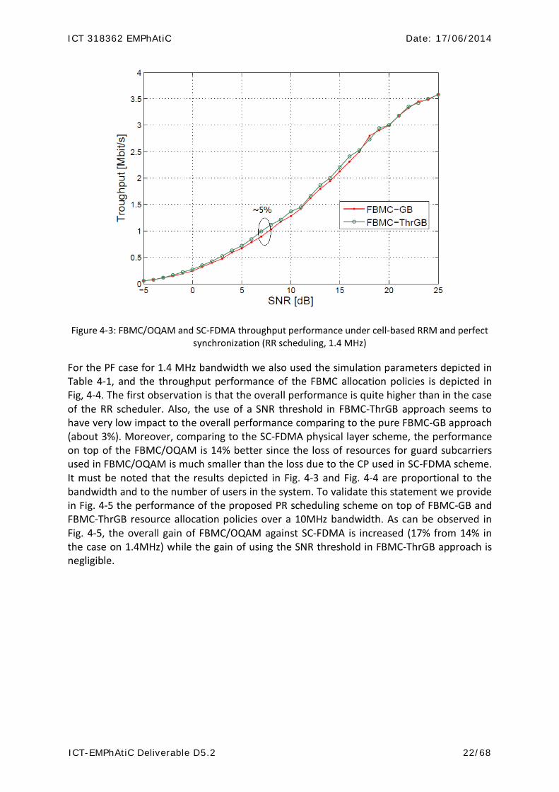
In this section, we extend the proposed scheduling scheme with a resource allocation policy applicable to the adopted physical layer scheme. Based on the result shown in Fig 4-2, for the FBMC/OQAM scheme two policies are defined: i) the FBMC-GB resource allocation policy, where the BS uses a guard subcarrier to protect transmissions of users transmitting in adjacent bands, and ii) the FBMC-ThrGB resource allocation policy, where the BS uses a guard subcarrier to protect transmissions of users transmitting in adjacent bands only when the SNR is above a predefined threshold. To exemplify the FBMC/OQAM performance under these resource allocation policies, we first apply them over a Round Robin (RR) scheduling scheme (Fig. 4-3) and then over the proposed PF scheme (Fig. 4-4 and Fig. 4-5). In Fig 4-3 we show the performance of RR scheduling for 1.4MHz bandwidth on top of two different PHY layer schemes: i) the FBMC/OQAM with the FBMC-GB policy ii) the FBMC/OQAM with the FBMC-ThGB policy, where the predefined threshold is equal to 12 dB. Using the simulation parameters shown in Table 4-1, the overall gain that is provided by the use of the SNR threshold is about 5%. Even if it is a quite low gain, it must be noticed that the maximum number of guard subcarriers that can be used in 1.4MHz bandwidth is 1/12=0,08 i.e., 8% of the total bandwidth, when each resource block is allocated to a different HH. Thus, the maximum achievable gain is 8%.
ICT 318362 EMPhAtiC Date: 17/06/2014
ICT-EMPhAtiC Deliverable D5.2 22/68
Figure 4-3: FBMC/OQAM and SC-FDMA throughput performance under cell-based RRM and perfect synchronization (RR scheduling, 1.4 MHz)
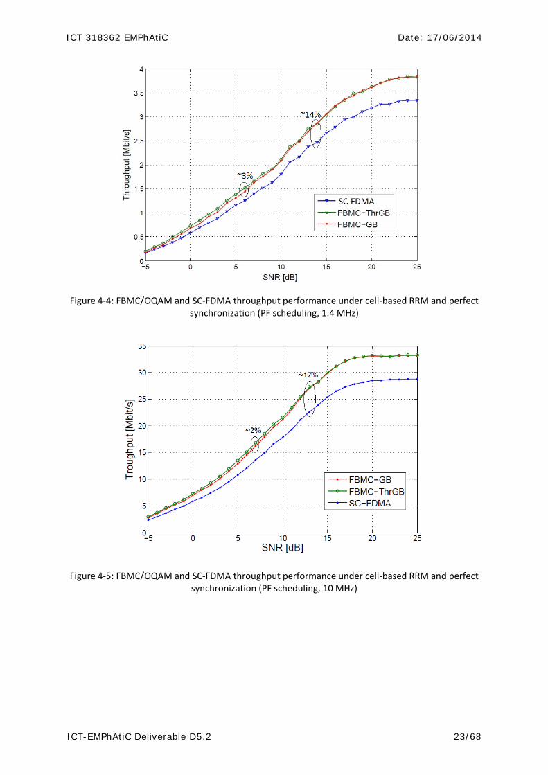
For the PF case for 1.4 MHz bandwidth we also used the simulation parameters depicted in Table 4-1, and the throughput performance of the FBMC allocation policies is depicted in Fig, 4-4. The first observation is that the overall performance is quite higher than in the case of the RR scheduler. Also, the use of a SNR threshold in FBMC-ThrGB approach seems to have very low impact to the overall performance comparing to the pure FBMC-GB approach (about 3%). Moreover, comparing to the SC-FDMA physical layer scheme, the performance on top of the FBMC/OQAM is 14% better since the loss of resources for guard subcarriers used in FBMC/OQAM is much smaller than the loss due to the CP used in SC-FDMA scheme. It must be noted that the results depicted in Fig. 4-3 and Fig. 4-4 are proportional to the bandwidth and to the number of users in the system. To validate this statement we provide in Fig. 4-5 the performance of the proposed PR scheduling scheme on top of FBMC-GB and FBMC-ThrGB resource allocation policies over a 10MHz bandwidth. As can be observed in Fig. 4-5, the overall gain of FBMC/OQAM against SC-FDMA is increased (17% from 14% in the case on 1.4MHz) while the gain of using the SNR threshold in FBMC-ThrGB approach is negligible.
ICT 318362 EMPhAtiC Date: 17/06/2014
ICT-EMPhAtiC Deliverable D5.2 23/68
Figure 4-4: FBMC/OQAM and SC-FDMA throughput performance under cell-based RRM and perfect synchronization (PF scheduling, 1.4 MHz)
Figure 4-5: FBMC/OQAM and SC-FDMA throughput performance under cell-based RRM and perfect synchronization (PF scheduling, 10 MHz)

ICT 318362 EMPhAtiC Date: 17/06/2014
ICT-EMPhAtiC Deliverable D5.2 24/68
5. Sum-Rate Maximization Approach This section considers the crisis scenario described in section 2.2.2.1 and solves the sum-rate maximization problem. As explained in the following, sum-rate maximization leads to the highest sum rate, at the expense of the lowest fairness among users. Max-sum rate is relevant in a PMR scenario in order to get an upper bound on the achievable data rate.
5.1 State of the art on sum-rate maximization When dealing with resource allocations, one of the most widely investigated criterion in the literature is the sum-rate capacity. The sum-rate criterion does not consider any fairness issue or rate constraint, but is a useful benchmark to compare with, since any other practical RRM policy will necessary yield a lower total sum-rate. Both the centralized (e.g., [14]) and the distributed approaches (e.g., [15]) have been widely investigated. In the centralized approach the allocation is decided and broadcasted by a central node (or fusion center) which has the entire network and environment information. In the distributed approach each node decides independently without having the network knowledge or exchanges limited information. In general what makes things very difficult is the interference between different links. Optimal algorithms for interference-limited sum-rate capacity have been only proposed in the late 2000 for the centralized cased and only very recently for the distributed case with limited exchanges. Interested readers can refer for example to [14, 15] and references therein (Note that we do not talk about the complexity of such algorithms). Although the algorithm proposed in [15] is distributed due to the asynchronous decision and message exchange, the amount of information exchanged is not negligible. In addition the Gibbs sampling approach proposed in [15] is not necessarily easy to use with continuous power and multi-channel, i.e., see the sum-integral to be computed for the continuous algorithm. Alternatively, for the continuous power problem [16] proposes a distributed approach (non-optimal) where approximations have been used to convexify the non-convex problem. Although so-called distributed, the algorithms proposed in [15] or [16] exhibit a large information exchange requirement, which may not be feasible in practice, especially for the clusterized ad-hoc scenarios investigated here. Therefore, we need to focus on other non-optimal works with more realistic information exchange. Interested readers can refer for example to [17] for a good overview of such state-of-the-art algorithms. The existing algorithms differ by their level of information exchange. It goes from the simplest case of no information exchange at all, to specific limited exchanges. We quickly present hereafter some key properties. For the approaches with no signaling exchanged, the only information known by a node about the environment indirectly comes from the total interference experienced at the reception (i.e., cumulated interference from all other links using the same resource). It has been shown in [18] that for such rate utilities the best response power allocation in the absence of information exchange is the distributed iterative waterfilling. The idea is for a given transmitter m to asynchronously and iteratively update its power by only considering the updated experienced interference (following the changes from other nodes allocation). At a given time instance t user m would need to optimize the following equivalent problem
( )
( ) ( )
2 ( )( )0
( ) ( )max log (1 )( )k
m
k km mm
kp tk m
p t g tN I t
++∑

ICT 318362 EMPhAtiC Date: 17/06/2014
ICT-EMPhAtiC Deliverable D5.2 25/68
where )(kmp is the transmission power of transmitter m on the k th RB, )(k
mmg is the channel power between the transmitter m and its respective receiver on the k th RB, 0N is the internal noise, and )(k
mI is the cumulated interference experienced by the m th receiver on the k th RB. This best response depends on the distribution of interference over RBs, which in turn is determined by power allocations at neighboring transmitters. Hence, a Nash equilibrium can be determined by an iterative waterfilling method in which users update their power allocations until the power allocations converge. The updates could occur sequentially in any order or synchronously. As explained in [17], for the P2P networks considered, a Nash equilibrium needs not to exist and even when one does exist, iterative waterfilling does not always converge. This is especially true when the cross-interference between the different links is too high. Yet, the iterative waterfilling has been widely used and adapted for different related allocation problems (e.g., [19] dealing with FBMC and OFDM RRM comparison).
For the approaches with limited exchanges, the algorithms vary with the available side-information as well as the exchange rate. Many algorithms have been proposed which are based on the iterative waterfilling but considering additional side-information added as a cost function in the utility function of interest, i.e.,
( )
( ) ( )( )
2 ( )( )0
( ) ( )max log (1 ) ( )( )k
m
k kkm mm
mkp tk m
p t g t tN I t
+ −Φ+∑
where )(tΦ is the cost function. As an example we can refer to ADP/MADP algorithms (Asynchronous Distributed Pricing / Multichannel ADP) proposed in [20]. The cost function at a given user m represents the cumulated interference generated by that user on all other users, i.e,
)()()()( )()()()( tgttpt kmj
mj
kj
km
km ∑
≠
=Φ χ
where )(
)(0
)()(
2)(
)1(log
km
kk
j
kjj
kj
kj I
INgp
∂
++∂
−=∑
χ . This approach requires each transmitter to know
)(kjχ for all other links, and needs to be updated after every RRM change.
The works mentioned above and therein generally focus on the sum-rate problem which provides a good theoretical benchmark to assess other more realistic RRM policies (i.e., QoS constraints). To equitably share the limited resource, fair utility functions can be used such as the alpha-fair function as proposed in [21] for the centralized problem. Achieving such fairness in a distributed way with limited information still needs investigations. Another type of criterion is the rate constraint problem as later investigated in Section 6. The idea is to minimize the power consumption such that each user’s minimum rate constraint is achieved, e.g., see [22] for the centralized problem (assuming the rates are feasible).
5.2 System model In this section, we study the sum-rate maximization on an instantaneous channel. According to the adopted crisis scenario (see section 2.2.2.1), the BSs as well as the MSs follow a
ICT 318362 EMPhAtiC Date: 17/06/2014
ICT-EMPhAtiC Deliverable D5.2 26/68
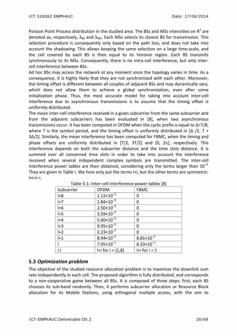
Poisson Point Process distribution in the studied area. The BSs and MSs intensities on R2 are denoted as, respectively, λBS and λMS. Each MSs selects its closest BS for transmission. This selection procedure is consequently only based on the path loss, and does not take into account the shadowing. This allows keeping the same selection on a large time-scale, and the cell covered by each BS is then equal to its Voronoi region. Each BS transmits synchronously to its MSs. Consequently, there is no intra-cell interference, but only inter-cell interference between BSs. Ad hoc BSs may access the network at any moment since the topology varies in time. As a consequence, it is highly likely that they are not synchronized with each other. Moreover, the timing offset is different between all couples of adjacent BSs and may dynamically vary, which does not allow them to achieve a global synchronization, even after some initialization phase. Thus, the most accurate model for taking into account inter-cell interference due to asynchronous transmissions is to assume that the timing offset is uniformly distributed. The mean inter-cell interference received in a given subcarrier from the same subcarrier and from the adjacent subcarriers has been evaluated in [8], when two asynchronous transmissions occur. It has been computed in OFDM when the cyclic prefix is equal to Δ=T/8, where T is the symbol period, and the timing offset is uniformly distributed in [Δ /2, T + 3Δ/2]. Similarly, the mean interference has been computed for FBMC, when the timing and phase offsets are uniformly distributed in [T/2, 3T/2] and [0, 2π], respectively. This interference depends on both the subcarrier distance and the time slots distance. It is summed over all concerned time slots in order to take into account the interference received when several independent complex symbols are transmitted. The inter-cell interference power tables are then obtained, considering only the terms larger than 10−3. They are given in Table I. We here only put the terms l+i, but the other terms are symmetric: l+i=l−i.
Table 5-1: Inter-cell interference power tables [8] Subcarrier OFDM FBMC l+8 1.12×10⁻³ 0 l+7 1.84×10⁻³ 0 l+6 2.50×10⁻³ 0 l+5 3.59×10⁻³ 0 l+4 5.60×10⁻³ 0 l+3 9.95×10⁻³ 0 l+2 2.23×10⁻² 0 l+1 8.94×10⁻² 8.81×10⁻² l 7.05×10⁻¹ 8.23×10⁻¹ l-i l+i for i = {1,8} l+i for i = 1
5.3 Optimization problem The objective of the studied resource allocation problem is to maximize the downlink sum rate independently in each cell. The proposed algorithm is fully distributed, and corresponds to a non-cooperative game between all BSs. It is composed of three steps: first, each BS chooses its sub-band randomly. Then, it performs subcarrier allocation or Resource Block allocation for its Mobile Stations, using orthogonal multiple access, with the aim to
ICT 318362 EMPhAtiC Date: 17/06/2014
ICT-EMPhAtiC Deliverable D5.2 27/68
maximize the cell sum rate. Finally, an iterative power allocation is used, where each BS performs water-filling on its subcarriers, considering the received sum interference as noise. The total bandwidth, Btot, is composed of L subcarriers, and the bandwidth of each subcarrier is denoted as Δf, with Δf= 15 kHz. Subcarriers are grouped in Resource Blocks of 12 consecutive subcarriers, thus forming a set of 180 kHz available for resource allocation. Let us assume that the Poisson Point Process has given NBS Base Stations. Let NMS k be the number of Mobile Stations served by the kth BS. Then 𝐺𝑘[𝑖],𝑗
𝑙 is the channel gain (including square fading, path loss and shadowing) between the jth BS and the ith Mobile Station served by BS k in subcarrier l. We first suppose that all the cells in the network share the same bandwidth Btot. Then, the Signal-to-Interference-plus-Noise-Ratio of this Mobile Station in subcarrier is:
𝑆𝐼𝑁𝑅𝑘[𝑖]𝑙 =
𝐺𝑘[𝑖],𝑘𝑙 𝑃𝑘𝑙
𝑛0 + ∑ �∑ 𝐺𝑘[𝑖],𝑗𝑙′ 𝑉|𝑙−𝑙′|𝑃𝑗𝑙
′min (𝑙+𝑆,𝐿)𝑙′=max (1,𝑙−𝑆) �𝑁𝐴𝑃
𝑗≠𝑘
where n0 is the noise power per subcarrier and 𝑃𝑘𝑙 is the transmit power of BS k in subcarrier l. 𝑉 = [𝑉0,𝑉1, … ,𝑉𝑆] is the interference weight vector. According to Table I, it is equal to:
VOFDM = {7.05 x 10⁻¹, 8.94x10⁻², 2.23x10⁻², 9.95×10⁻³, 5.60×10⁻³, 3.59×10⁻³, 2.50×10⁻³, 1.84×10⁻³ ,1.12×10−3 }
VFBMC = {8.23×10⁻¹, 8.81×10⁻²}
VPS= {1}
with OFDM, FBMC and perfect synchronization (PS), respectively. Interference spreads over 17 subcarrier (since S=8) with OFDM, 3 subcarriers with FBMC (S=1), and one subcarrier with perfect synchronization, as in that case only co-channel interference occurs. Let 𝑎𝑘[𝑖],𝑘
𝑙 be the subcarrier allocation indicator, which is equal to 1 if the ith Mobile Station served by BS k is allocated in subcarrier l, and 0 otherwise. Then the optimization problem at BS k (assuming that NMS[k] >0) can be written as:
𝑚𝑎𝑥𝒂𝑘,𝑷𝑘 ∑ ∑ 𝑎𝑘[𝑖],𝑘𝑙𝐿
𝑙=1𝑁𝑀𝑆[𝑘]𝑖=1 𝑙𝑜𝑔2�1 + 𝑆𝐼𝑁𝑅𝑘[𝑖]
𝑙 � (5.1)
𝑠. 𝑡. � 𝑎𝑘[𝑖],𝑘𝑙 ≤ 1 ∀ 𝑙 ∈ {1, … , 𝐿}
𝑁𝑀𝑆[𝑘]
𝑖=1
𝑠. 𝑡.�𝑃𝑘𝑙 ≤ 𝑃𝑚𝑎𝑥
𝐿
𝑙=1
𝑠. 𝑡. 𝑃𝑘𝑙 ≥ 0 ∀ 𝑙 ∈ {1, … , 𝐿}
ICT 318362 EMPhAtiC Date: 17/06/2014
ICT-EMPhAtiC Deliverable D5.2 28/68
Each BS performs resource allocation in order to solve problem (5.1), for a given level of interference. The proposed resource allocation algorithm is detailed in the next section.
5.4 Sum-rate maximization algorithm The proposed algorithm for sum-rate maximization is composed of three steps:
1. Sub-bands allocation per BS; 2. Subcarrier allocation or Resource Block allocation per BS; 3. Iterative power allocation.
We consider one channel realization, and assume that the channel varies slowly enough to be constant during the iterative power allocation.
5.4.1 Sub-bands allocation In order to mitigate inter-cell interference, the total bandwidth Btot is uniformly divided into NB sub-bands. Each sub-band contains nSB subcarriers. Then each BS randomly chooses one of the sub-bands, with equal probability for each sub-band. We denote by Bk the sub-band allocated to BS k. Since this allocation is totally random, it is likely that some adjacent cells in the ad hoc network will get the same sub-band.
5.4.2 Subcarrier allocation Subcarrier allocation is performed independently per BS, assuming equal power allocation per subcarrier, Pl,k=Pmax/L. Let us consider BS k, that operates in sub-band Bk. In the following, we assume that the number of subcarriers per sub-band, nSB, is always higher than 8. Consequently, even with OFDM, the inter-cell interference received in subcarrier l is only due to the cells that operate either in the same sub-band Bk, or in the adjacent sub-bands, Bk−1 and Bk+1. The SINR for user k[i] can be simplified as:
𝑆𝐼𝑁𝑅𝑘[𝑖]𝑙 =
𝐺𝑘[𝑖],𝑘𝑙 𝑃𝑘𝑙
𝑛0 + 𝐼𝑘[𝑖],𝑡𝑜𝑡𝑙
where 𝐼𝑘[𝑖],𝑡𝑜𝑡𝑙 = ∑ 𝐼𝑘[𝑖],𝑗
𝑙𝑁𝐴𝑃𝑗:𝑗≠𝑘; 𝐵𝑗=𝐵𝑘 + ∑ 𝐼𝑘[𝑖],𝑗
𝑙𝑁𝐴𝑃𝑗:𝑗≠𝑘; 𝐵𝑗=𝐵𝑘−1 + ∑ 𝐼𝑘[𝑖],𝑗
𝑙𝑁𝐴𝑃𝑗:𝑗≠𝑘; 𝐵𝑗=𝐵𝑘+1
𝐼𝑘[𝑖],𝑡𝑜𝑡𝑙 = � 𝐼𝑘[𝑖],𝑗
𝑙
𝑁𝐴𝑃
𝑗:𝑗≠𝑘; 𝐵𝑗=𝐵𝑘
+ � 𝐼𝑘[𝑖],𝑗𝑙
𝑁𝐴𝑃
𝑗:𝑗≠𝑘; 𝐵𝑗=𝐵𝑘−1
+ � 𝐼𝑘[𝑖],𝑗𝑙
𝑁𝐴𝑃
𝑗:𝑗≠𝑘; 𝐵𝑗=𝐵𝑘+1
𝐼𝑘[𝑖],𝑗𝑙 is the interference received from the same sub-band, that can spread over a maximum
of 2S+1 subcarrier (depending on the location of subcarrier l), and includes the interference from subcarrier l. 𝐼𝑘[𝑖],𝑗
𝑙 is the interference received from the previous sub-band, and 𝐼𝑘[𝑖],𝑗𝑙
is the interference received from the next sub-band. Both of them can spread over a maximum of S subcarrier, if there is no guard band. In details, we obtain:
𝐼𝑘[𝑖],𝑗𝑙 = � 𝐺𝑘[𝑖],𝑗
𝑙′ 𝑉�𝑙−𝑙′�𝑃𝑗𝑙′
min (𝑙+𝑆,𝐵𝑘[𝑛𝑆𝐵])
𝑙′=max (𝐵𝑘[1],𝑙−𝑆)
where Bk [p] is the pth subcarrier of the sub-band allocated to BS k. Similarly,
ICT 318362 EMPhAtiC Date: 17/06/2014
ICT-EMPhAtiC Deliverable D5.2 29/68
𝐼𝑘[𝑖],𝑗𝑙 = � 𝐺𝑘[𝑖],𝑗
𝑙′ 𝑉�𝑙−𝑙′�𝑃𝑗𝑙′
𝐵𝑗[𝑛𝑆𝐵]
𝑙′=max (𝐵𝑗[1],𝑙−𝑆)
and
𝐼𝑘[𝑖],𝑗𝑙 = � 𝐺𝑘[𝑖],𝑗
𝑙′ 𝑉�𝑙−𝑙′�𝑃𝑗𝑙′
min (𝑙+𝑆,𝐵𝑗[𝑛𝑆𝐵])
𝑙′=𝐵𝑗[1]
Please note that 𝐼𝑘[𝑖],𝑗𝑙 or 𝐼𝑘[𝑖],𝑗
𝑙 may be equal to 0, if the sets for the sums are empty. In order to maximize the sum rate, each subcarrier in Bk is allocated to the Mobile Station with the highest SINR. The allocation rule is:
𝑎𝑘[𝑖],𝑘𝑙 = 1 𝑖𝑓 𝑘[𝑖] = arg𝑚𝑎𝑥𝑖=�1,..,𝑁𝑀𝑇[𝑘]� 𝑆𝐼𝑁𝑅𝑘[𝑖]
𝑙
𝑎𝑘[𝑖],𝑘𝑙 = 0 𝑜𝑡ℎ𝑒𝑟𝑤𝑖𝑠𝑒
In the following, we denote by ul,k the Mobile Station allocated by BS k in subcarrier l. If subcarriers are allocated at the Resource Block level, then the average SINR per Resource Block is computed. The allocation rule is similar, with the exception that is takes the per-Resource Block SINR into account.
5.4.3 Iterative power allocation Once subcarriers have been allocated, the optimization problem (5.1) simplifies to:
𝑚𝑎𝑥𝑃𝑘 ∑ 𝑙𝑜𝑔2 �1 + 𝑏𝑢𝑘𝑙 ,𝑘𝑙 𝑃𝑘𝑙�𝐿
𝑙=1 (5.2)
𝑠. 𝑡.�𝑃𝑘𝑙 ≤ 𝑃𝑚𝑎𝑥
𝐿
𝑙=1
𝑠. 𝑡. 𝑃𝑘𝑙 ≥ 0 ∀ 𝑙 ∈ {1, … , 𝐿}
where 𝑏𝑢𝑘𝑙 ,𝑘𝑙 =
𝐺𝑢𝑘𝑙 ,𝑘𝑙
𝑛0+𝐼𝑢𝑘𝑙 ,𝑡𝑜𝑡𝑙
The problem described in (5.2) is convex and is solved by water-filling over the subcarriers. The analytical solution is:
𝑃𝑘𝑙 = � 1𝜇𝑘− 1
𝑏𝑢𝑘𝑙 ,𝑘
𝑙 �+
(5.3)
where [𝑥]+ = 𝑚𝑎𝑥{𝑥, 0} and 𝜇𝑘 is a constant set in order to fulfill the constraint ∑ 𝑃𝑘𝑙 = 𝑃𝑚𝑎𝑥𝐿𝑙=1 .
The solution of problem (5.2) is provided for a given level of interference. On the whole ad hoc network, power allocation is performed using iterative water-filling. During an iterative
ICT 318362 EMPhAtiC Date: 17/06/2014
ICT-EMPhAtiC Deliverable D5.2 30/68
phase, each Mobile Station measures the level of interference that it receives from the other cells per subcarrier. Then, it feeds back this value to its Base Station. The feedback procedure is assumed perfect. Finally, the BS updates its transmit power values according to eq. (5.3). This procedure is performed in each cell independently and in parallel. Of course, we cannot prove that it converges, since this is a modified version of iterative water-filling, whose convergence is not theoretical but practical, when the number of subcarriers is large enough [9]. Yet, numerical simulations show a very fast convergence of the algorithm to a stable state.
5.5 Performance evaluation The performances of the proposed algorithm are evaluated using Monte-Carlo simulations. The path loss model is ITU-R P1411-4 [10], for propagation between terminals located below roof-top height at UHF, with fc = 770 MHz, and a location percentage set to p = 90%. The shadowing’s standard deviation is equal to 9 dB and the fading follows a Rayleigh distribution. An area of 20 km2 is chosen and the BS density is λBS=1. Consequently, there are in average 20 BS in the considered area.
The maximum transmit power per BS is Pmax=43 dBm, and the BS antenna gain plus cable loss is equal to 14 dBi. The Mobile Station’s antenna gain plus cable loss is assumed equal to 0 dBi. The subcarrier bandwidth is equal to Δf=15 kHz. The thermal noise has a spectral density of −174 dBm/Hz.
Two PMR configurations are tested: 1. Btot=5 MHz, with L=300 useful subcarriers in total. Consequently, there are 25
Resource Blocks. The number of sub-bands is NB=8, and each sub-band contains 3 adjacent Resource Blocks.
2. Btot=1.4 MHz, with L=72 useful subcarriers in total. Consequently, there are 6 Resource Blocks. The number of sub-bands is NB=6, and each sub-band contains 1 a Resource Block.
We compare the performances obtained with the proposed resource allocation algorithm, with FBMC and OFDM. In order to have an upper bound, we also evaluate the performances obtained with perfect synchronization, i.e., when interference only comes from the same subcarrier. This case is denoted as ’PS’ on the figures. It should be noted that the spectral efficiencies given afterwards are raw spectral efficiencies, which are also equal to the effective spectral efficiency for PS and FBMC. However, the effective spectral efficiency for OFDM is equal to 8/9th of the raw spectral efficiency, since the cyclic prefix is set to Δ=T/8.
In the following, we first provide the data rates achieved when subcarrier allocation is performed at the subcarrier level; then we compare these results when subcarrier allocation is performed at the Resource Block level. In that second case, the SINR per Resource Block is computed as the average SINR on the 12 subcarriers composing the Resource Block. Even though per-subcarrier allocation is not feasible in practical PMR, these results allow us to evaluate the rate loss due to Resource Block allocation.
ICT 318362 EMPhAtiC Date: 17/06/2014
ICT-EMPhAtiC Deliverable D5.2 31/68
5.5.1 Data rate with Btot=5 MHz
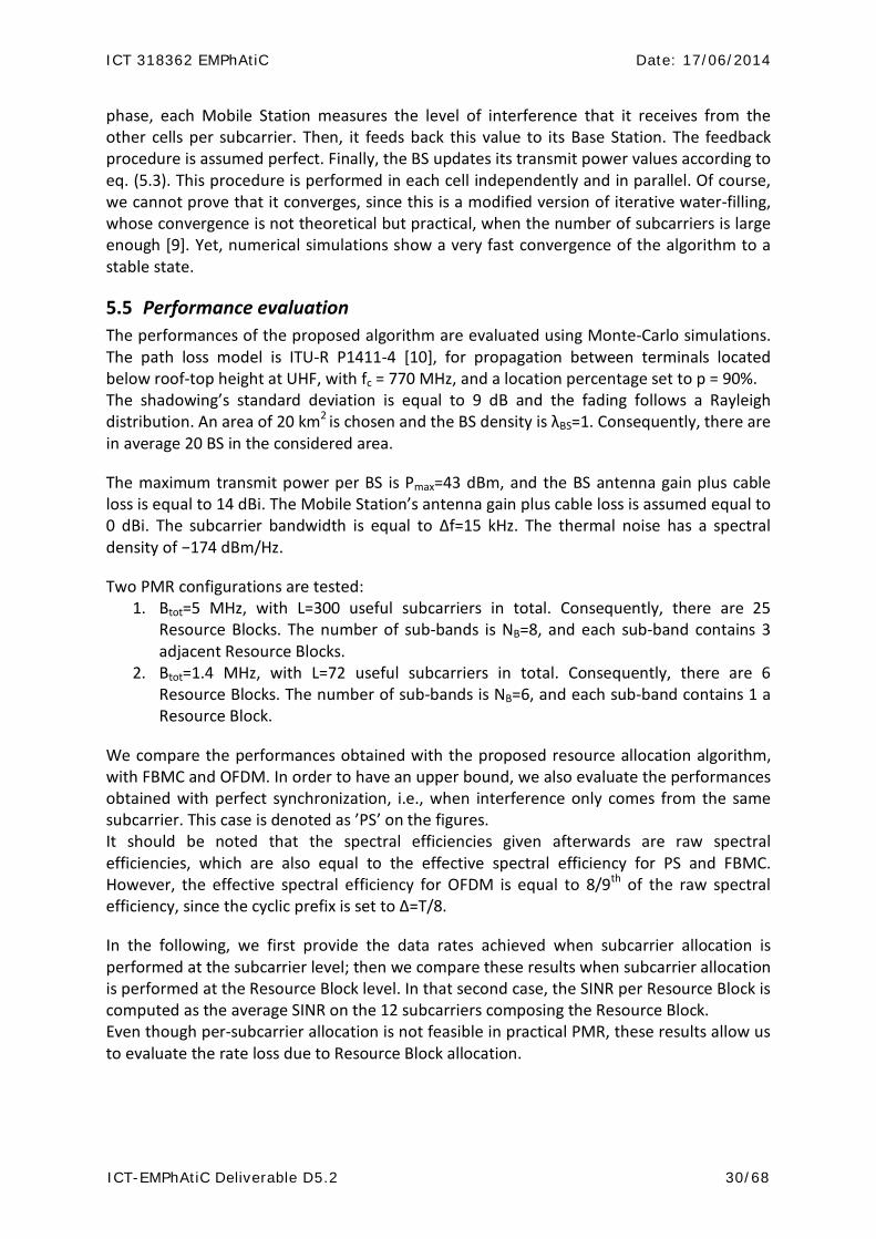
Figure 5-1: Sum rate with per-subcarrier allocation and Btot= 5 MHz
The sum rate is higher with FBMC than with OFDM. With per-subcarrier allocation, the sum rate relative decrease, compared to the optimal perfect synchronization case, is between 7.1 and 7.7 % with FBMC, and between 12.4 and 14.2 % with OFDM. With per RB allocation, all sum rates are decreased of 9 to 20%, whatever the multi-carrier modulation. The rate decrease is higher when the MSs density increases, since the influence of the diversity decrease due to per-RB allocation is more important at high load.

ICT 318362 EMPhAtiC Date: 17/06/2014
ICT-EMPhAtiC Deliverable D5.2 32/68
5.5.2 Data rate with Btot=1.4 MHz
Figure 5-1: Sum rate with per-subcarrier allocation and Btot = 1.4 MHz
Figure 5-2: Sum rate with per-RB allocation and Btot = 1.4 MHz
Similar conclusions stand when Btot = 1.4 MHz. The sum rate is still higher with FBMC than with OFDM. With per-subcarrier allocation, the sum rate relative decrease, compared to the optimal perfect synchronization case, is between 8.1 and 9.8% with FBMC, and between 15.7 and 19.8% with OFDM.

ICT 318362 EMPhAtiC Date: 17/06/2014
ICT-EMPhAtiC Deliverable D5.2 33/68
With per RB allocation, all sum rates are decreased of 10 to 19%, whatever the multi-carrier modulation. We can notice that in the latter case, the average rate per BS is 1.2 to 2.00 MHz with FBMC. This rate seems reasonable for PMR applications.
ICT 318362 EMPhAtiC Date: 17/06/2014
ICT-EMPhAtiC Deliverable D5.2 34/68
6. Rate Adaptive Approach This section considers the crisis scenario described in section 2.2.2.1 and solves rate-adaptive allocation optimization problem with a distributed algorithm. Rate-adaptive allocation is the fairest resource allocation objective, since all users obtain the same data rate; but this fairness is achieved at the expense of low sum rate. For PMR applications, it is necessary to be able to achieve a minimum data rate for each MS/HH wherever its location. This constraint is taken into account in the proposed rate-adaptive resource allocation algorithm.
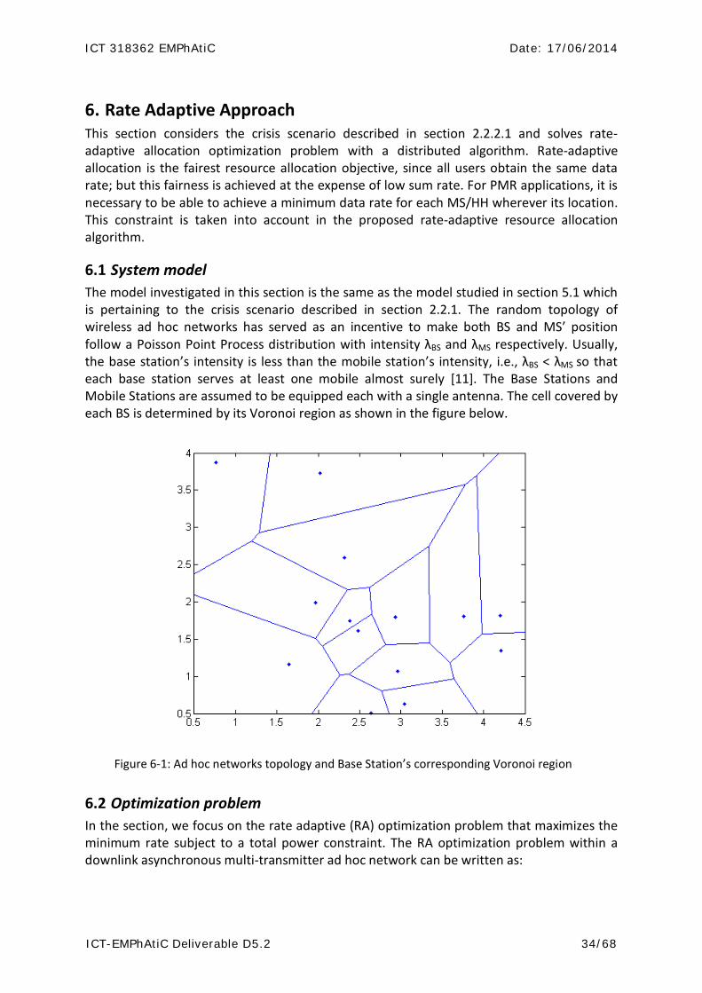
6.1 System model The model investigated in this section is the same as the model studied in section 5.1 which is pertaining to the crisis scenario described in section 2.2.1. The random topology of wireless ad hoc networks has served as an incentive to make both BS and MS’ position follow a Poisson Point Process distribution with intensity λBS and λMS respectively. Usually, the base station’s intensity is less than the mobile station’s intensity, i.e., λBS < λMS so that each base station serves at least one mobile almost surely [11]. The Base Stations and Mobile Stations are assumed to be equipped each with a single antenna. The cell covered by each BS is determined by its Voronoi region as shown in the figure below.
Figure 6-1: Ad hoc networks topology and Base Station’s corresponding Voronoi region
6.2 Optimization problem In the section, we focus on the rate adaptive (RA) optimization problem that maximizes the minimum rate subject to a total power constraint. The RA optimization problem within a downlink asynchronous multi-transmitter ad hoc network can be written as:
ICT 318362 EMPhAtiC Date: 17/06/2014
ICT-EMPhAtiC Deliverable D5.2 35/68
max𝒂𝑘,𝑷𝑘min � �𝑎𝑘[𝑖],𝑘𝑙
𝐿
𝑙=1
𝑁𝑀𝑆[𝑘]
𝑖=1
log2�1 + 𝑆𝐼𝑁𝑅𝑘[𝑖]𝑙 �
𝑠. 𝑡. � 𝑎𝑘[𝑖],𝑘𝑙 ≤ 1 ∀ 𝑙 ∈ {1, … , 𝐿}
𝑁𝑀𝑆[𝑘]
𝑖=1
�𝑃𝑘𝑙 ≤ 𝑃𝑚𝑎𝑥
𝐿
𝑙=1
𝑃𝑘𝑙 ≥ 0 ∀ 𝑙 ∈ {1, … , 𝐿}
It was shown in [12] that the RA optimization problem can be decomposed into iterative Margin Adaptive (MA) optimization problems. Basically, the MA optimization minimizes the total power consumption while ensuring each user received rate constraint is satisfied. The MA optimization problem is formulated as
min𝒂𝑘,𝑷𝑘�𝑎𝑘[𝑖],𝑘 𝑙
𝐿
𝑙=1
𝑃𝑘𝑙
s.t. RTarget ≤ ∑ 𝑎𝑘[𝑖],𝑘
𝑙𝐿𝑙=1 log2�1 + 𝑆𝐼𝑁𝑅𝑘[𝑖]
𝑙 � ∀ 𝑖 ∈ �1, … ,𝑁𝑀𝑆[𝑘]� ∑ 𝑎𝑘[𝑖],𝑘
𝑙 ≤ 1 ∀ 𝑙 ∈ {1, … , 𝐿}𝑁𝑀𝑆[𝑘]𝑖=1
�𝑃𝑘𝑙 ≤ 𝑃𝑚𝑎𝑥
𝐿
𝑙=1
𝑃𝑘𝑙 ≥ 0 ∀ 𝑙 ∈ {1, … , 𝐿}
In order to tackle the computational complexity of the MA optimization problem, a suboptimal resource allocation scheme that solves the problem during two steps can be adopted. First of all, subcarrier allocation is performed using the scheme proposed in [13]. Secondly, power allocation is performed assuming subcarrier allocation is done.
Suppose that subcarrier allocation known, we focus on proposing a general distributed convergence criterion to be fulfilled by distributed power allocation scheme to converge. Distributed MA algorithms may not converge if inter-cell interference is too high. To avoid that problem, a general convergence criterion fit for any multi-carrier modulation is investigated. The general convergence criterion is summarized in the following lemma.
Lemma Any distributed power control algorithm for multi-cell asynchronous ad hoc networks satisfying
𝛾𝑢(𝑘,𝑙)𝑙 �∑ ∑ 𝐺𝑘[𝑖],𝑗
𝑙′ 𝑉�𝑙−𝑙′�𝑙′∈𝐿𝑗≠𝑘 �
𝐺𝑢(𝑘,𝑙)𝑙 < 1 ∀ 𝑙 ∀ 𝑘
converges. In the previous expression, 𝛾𝑢(𝑘,𝑙)𝑙 represents the target SINR for user 𝑢 that was
assigned the 𝑙-th subcarrier by its serving Base Station 𝑘. Also, 𝐿 denotes the set of all interferences.
ICT 318362 EMPhAtiC Date: 17/06/2014
ICT-EMPhAtiC Deliverable D5.2 36/68
The power allocation for the MA optimization problem is done by taking into account the aforementioned convergence criterion. A distributed power control algorithm executed in a round robin fashion among the Base Stations is adopted.
When optimality is reached, all constraints will be tight. Therefore, within a subcarrier, at optimality
𝑃𝑘𝑙 =𝛾𝑢(𝑘,𝑙)𝑙 �𝑛0 + ∑ ∑ 𝐺𝑘[𝑖],𝑗
𝑙′ 𝑉�𝑙−𝑙′�𝑃𝑗𝑙′
𝑙′∈𝐿𝑗≠𝑘 �
𝐺𝑢(𝑘,𝑙)𝑙 ∀ 𝑙 ∀ 𝑘
To further simplify the notation, let
𝐼𝑘𝑙 =�𝑛0 + ∑ ∑ 𝐺𝑘[𝑖],𝑗
𝑙′ 𝑉�𝑙−𝑙′�𝑃𝑗𝑙′
𝑙′∈𝐿𝑗≠𝑘 �
𝐺𝑢(𝑘,𝑙)𝑙
𝐶𝑘𝑙 =𝐺𝑢(𝑘,𝑙)𝑙
∑ ∑ 𝐺𝑘[𝑖],𝑗𝑙′ 𝑉|𝑙−𝑙′|𝑙′∈𝐿𝑗≠𝑘
Therefore, for the 𝑘-th Base Station, the power allocation of the MA optimization problem is equivalent to
min𝛾𝑖�𝛾𝑘,𝑢(𝑘,𝑙)𝑙
𝐿
𝑙=1
𝐼𝑘𝑙
s.t. RTarget ≤� log2�1 + 𝛾𝑖𝑙�𝑛𝑐𝑖
𝑙=1
∀ 𝑖 ∈ �1, … ,𝑁𝑀𝑆[𝑘]�
𝛾𝑘𝑙 ≤ 𝐶𝑘𝑙 + 𝜖1 𝛾𝑘𝑙 ≥ 0 ∀ 𝑙 ∈ {1, … , 𝐿}
Where for each user i , nci is the number of subcarriers allocated by its serving Base Station. Also 𝜖1 is an infinitesimal positive constant added to satisfy the strict inequality of the convergence criterion. The previous optimization problem is a convex optimization problem and it can be efficiently solved using standard convex solver such as cvx.
6.3 Proposed resource allocation algorithm
In order to solve the RA optimization problem, the above MA power control optimization problem is solved. Since the total power constraint was not embedded into the above MA optimization problem, it is compulsory to verify after convergence whether or not the total power constraint per Base Station is met and update the target rate accordingly. The proposed algorithm is summarized as follows:
ICT 318362 EMPhAtiC Date: 17/06/2014
ICT-EMPhAtiC Deliverable D5.2 37/68
6.4 Simulation results In this section, numerical results for the downlink margin adaptive problem are provided. These numerical analyses highlight the performance of the distributed convergence criterion. The numerical results are conducted using Monte Carlo simulations.
Channel realizations between the BSs and MSs are assumed to be i.i.d Rayleigh fading with the path loss model ITU-R P1411-4 [10], and for propagation between terminals located below roof-top height at UHF, with fc = 770 MHz. Furthermore, in the simulations, the shadowing's is equal to 9 dB. The total area of communication is imposed to be 20 km2. Unless stated otherwise the BS density is λBS=1.
The transmit power mask per BS is chosen to be Pmax=43 dBm. The Base Station’s antenna gain plus cable loss is equal to 14 dBi while the loss in assumed to be negligible for the MSs. The total number of subcarriers is 72 with a bandwidth of 15 kHz each. Δ is equal to 4 Kbits/s and 𝜖1 is chosen to be 10-8. The thermal noise has a spectral density of −174 dBm/Hz.

ICT 318362 EMPhAtiC Date: 17/06/2014
ICT-EMPhAtiC Deliverable D5.2 38/68
Figure 6-2: Convergence curve versus number of iterations for λBS=1 and λMS=8
The performance and convergence properties of the proposed are examined in Figure 6-2 under different multi-carrier modulation schemes: FBMC and OFDM. In order to find a benchmark for our result, we also compare with the perfect synchronization case denoted as PS. Figure 6-2 shows the convergence behavior of iterative power allocation of the proposed algorithm for a fixed user rate RTarget = 64 kbits/s. Figure 6-2 shows that the algorithm converges regardless of the multi-carrier modulation technique utilized. Moreover, we also observe that the proposed algorithm converges faster when FBMC is used if compared to OFDM.
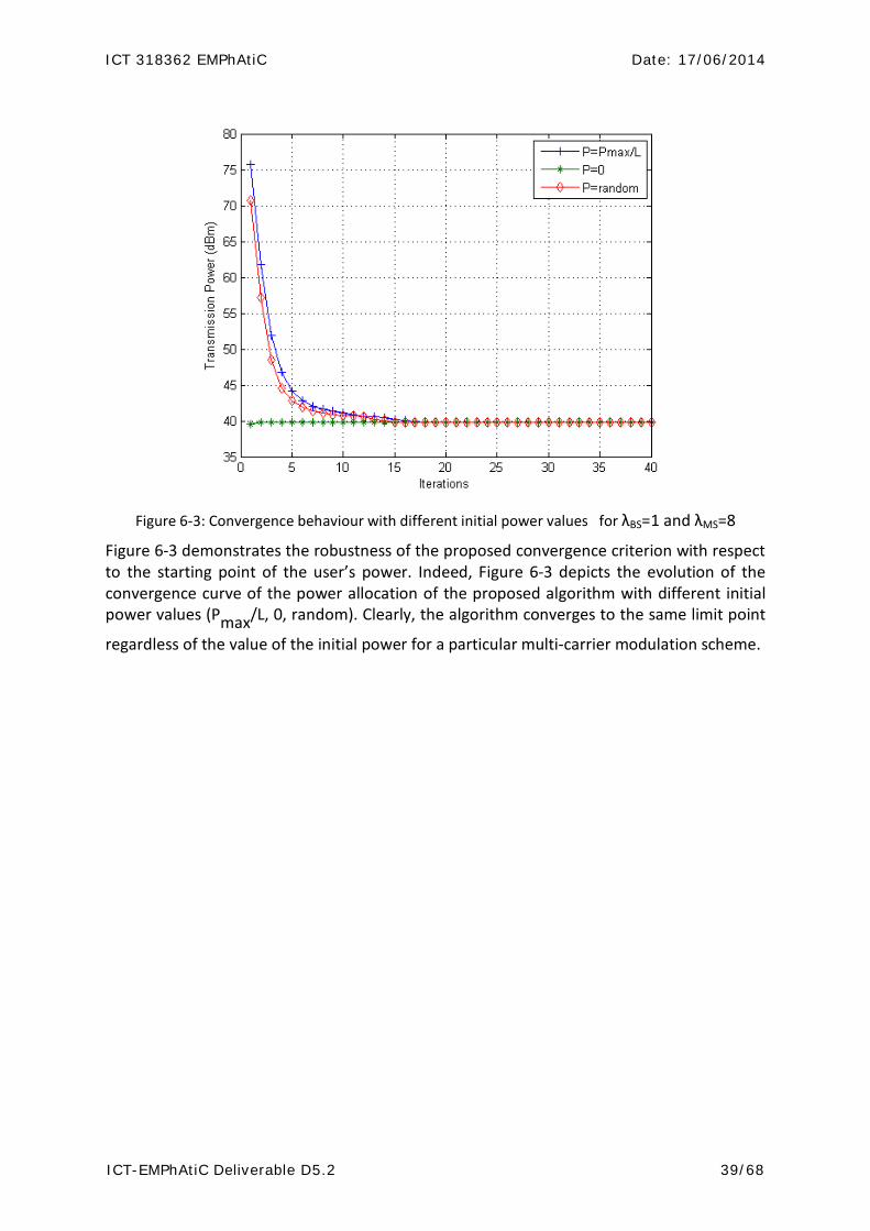
ICT 318362 EMPhAtiC Date: 17/06/2014
ICT-EMPhAtiC Deliverable D5.2 39/68
Figure 6-3: Convergence behaviour with different initial power values for λBS=1 and λMS=8
Figure 6-3 demonstrates the robustness of the proposed convergence criterion with respect to the starting point of the user’s power. Indeed, Figure 6-3 depicts the evolution of the convergence curve of the power allocation of the proposed algorithm with different initial power values (Pmax/L, 0, random). Clearly, the algorithm converges to the same limit point
regardless of the value of the initial power for a particular multi-carrier modulation scheme.
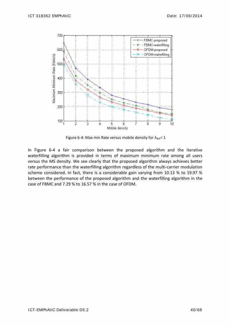
ICT 318362 EMPhAtiC Date: 17/06/2014
ICT-EMPhAtiC Deliverable D5.2 40/68
Figure 6-4: Max min Rate versus mobile density for λBS=1
In Figure 6-4 a fair comparison between the proposed algorithm and the iterative waterfilling algorithm is provided in terms of maximum minimum rate among all users versus the MS density. We see clearly that the proposed algorithm always achieves better rate performance than the waterfilling algorithm regardless of the multi-carrier modulation scheme considered. In fact, there is a considerable gain varying from 10.13 % to 19.97 % between the performance of the proposed algorithm and the waterfilling algorithm in the case of FBMC and 7.29 % to 16.57 % in the case of OFDM.

ICT 318362 EMPhAtiC Date: 17/06/2014
ICT-EMPhAtiC Deliverable D5.2 41/68
7. Data Buffer Stabilization Approach
7.1 System definition and assumptions
The RRM approach proposed in this section addresses the general clusterized ad-hoc scenario presented in Section 2.2.2.2. The key characteristics of the scenarios handled by the proposed algorithm are as follows: M total links N clusters (dynamic construction) K total resource blocks, with equivalent bandwidth Each cluster n is only affected a sub-set nK ( [ ]KK n ,1∈ ) (e.g., initially pre-allocated
in a complete random fashion but adapting in time with some learning process approach, see later Section 7.4.4 for more details)
In each cluster, the CH decides the allocation for all the internal communications; the allocations are orthogonal, i.e., only one link can be scheduled in a given RB such that no intra-cluster interference exists.
Each node has data buffer queue whose input bits are stochastic. Each CH broadcasts at different time interval the cumulated buffer size (of all
associated links), in a random fashion, i.e., collisions may occur if two nearby clusters transmit at the same time.
For the sake of simplicity we assume the following: In order to facilitate the analysis, we assume a time-slotted system (i.e., discrete
time t, representing for example a second). During the whole simulation, each of the M total links is always represented by the
same transmitter and its respective receiver, i.e., static traffic mapping without considering multiple possible receivers to be scheduled.
All nodes within a cluster receive without any loss all internal control or feedback information (e.g., allocation decision from the CH to all associated nodes, or link channel state from a node to its CH).
All CHs receive without loss the broadcast from any other CH (the case with loss due to collision is discussed in Section 7.6).
The capacity of a given node is modeled by the basic Shannon capacity (i.e., )1log( SINR+ ). We do not define any MCS.
It can be argued that those simplifications may have important impacts on the performance in real systems. Some possible adaptations are discussed in the conclusion part in section 7.6.
7.2 Literature review and motivations
7.2.1 Classical approaches and limitations Whether it is the sum-rate problems as investigated in Section 5 (see the literature review in Section 5.1), the fairness, or the rate-constraint problems as in Section 6, the usual optimization problem is a one shot/static type problem, i.e., it optimizes a unique
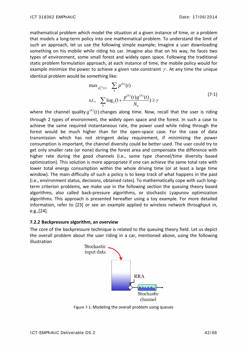
ICT 318362 EMPhAtiC Date: 17/06/2014
ICT-EMPhAtiC Deliverable D5.2 42/68
mathematical problem which model the situation at a given instance of time, or a problem that models a long-term policy into one mathematical problem. To understand the limit of such an approach, let us use the following simple example; Imagine a user downloading something on his mobile while riding his car. Imagine also that on his way, he faces two types of environment, some small forest and widely open space. Following the traditional static problem formulation approach, at each instance of time, the mobile policy would for example minimize the power to achieve a given rate constraint γ . At any time the unique identical problem would be something like:
( )( )
( )
( ) ( )
20
max ( )
( ) ( ). ., log (1 )
km
kp t
kk k
k
p t
p t g ts tN
γ+ ≥
∑
∑ ( 7-1)
where the channel quality )()( tg k changes along time. Now, recall that the user is riding through 2 types of environment, the widely open space and the forest. In such a case to achieve the same required instantaneous rate, the power used while riding through the forest would be much higher than for the open-space case. For the case of data transmission which has not stringent delay requirement, if minimizing the power consumption is important, the channel diversity could be better used. The user could try to get only smaller rate (or none) during the forest area and compensate the difference with higher rate during the good channels (i.e., some type channel/time diversity based optimization). This solution is more appropriate if one can achieve the same total rate with lower total energy consumption within the whole driving time (or at least a large time window). The main difficulty of such a policy is to keep track of what happens in the past (i.e., environment status, decisions, obtained rates). To mathematically cope with such long-term criterion problems, we make use in the following section the queuing theory based algorithms, also called back-pressure algorithms, or stochastic Lyapunov optimization algorithms. This approach is presented hereafter using a toy example. For more detailed information, refer to [23] or see an example applied to wireless network throughput in, e.g.,[24].
7.2.2 Backpressure algorithm, an overview The core of the backpressure technique is related to the queuing theory field. Let us depict the overall problem about the user riding in a car, mentioned above, using the following illustration
Figure 7-1: Modeling the overall problem using queues

ICT 318362 EMPhAtiC Date: 17/06/2014
ICT-EMPhAtiC Deliverable D5.2 43/68
A BS data buffer (queue) receives random inputs that need to be transmitted over the wireless stochastic channel to the moving node by controlling the RRM policy. Denote the queue’s input by )(ta and the output rate by )(tµ . The output rate is dependent on the RRM policy (i.e., how much transmission power, resource blocks, etc.) as well as the channel quality. It is easy to see that the queue dynamic, )(tq , can be expressed as
[ ] )()()1()( tattqtq +−−= +µ ( 7-2) where [ ] )0,max(xx =+ .This queue description models the fact that the incoming data increases the queue size while the transmitted data reduces it. In addition, [ ]+• operation guarantees that one cannot transmit more than what is currently in the queue. Observe that the mathematical queue is always positive or null. Imagine that this scenario is run for an infinite time period and assume that the buffer is theoretically unlimited. The optimal policy to minimize the overall transmission energy should intuitively yield the average input rate just equal to the average output rate. The problem can be formalized as follows (for the case of one user)
( ) ,min
. .,p t P t p
s t r µ∈ ∀
= ( 7-3)
where p , r , u represent the time-average transmit power, the time-average received bits in the buffer, and the time-average transmitted bits, respectively. Having defined the toy example setting and formulation, we now briefly present the key steps to design the RRM algorithm based on the backpressure framework:
a) Let ))(( tqL be any non-negative scalar valued function, called the Lyapunov function. A common function that has been hitherto used is the quadratic formulation
)(21))(( 2 tqtqL = , where )(tq is the buffer queue.
b) The expected multiple K-steps conditional Lyapunov drift is defined as { }))(())(()),(( tqLTtqLEttq −+=∆ | )(tq , where the expectation is taken over the
potential randomness of the channel state and control decision during the slot, given the current backlog (queue) state. Note that for the i.i.d channels, the analysis are performed using 1=K , whereas a channel with memory (e.g., Markov based) requires a multiple-step drift analysis (i.e., 1>K ).
c) An upper-bound for the expected Lyapunov drift is obtained. Note that the art of this stochastic optimal framework is designing a strategy to ensure the drift to be bounded.
d) The RRM policy is obtained from that upper-bound combined with some cost function (i.e., the problem objective function). It yields something similar to the following problem
( )max ( ) ( ( )) ( ( ))p t q t p t f p tµ η− ( 7-4)
ICT 318362 EMPhAtiC Date: 17/06/2014
ICT-EMPhAtiC Deliverable D5.2 44/68
whereη is a tunable constant, )(tq is the buffer queue defined earlier, and ))(( tpf is cost function based on the power. The positive part is the individual rate µ weighted by its own buffer queue size q , and the second part represents some cost relative to the power expenditure. It is important to note that it is thanks to the queue )(tq that the past actions and results are indirectly known.
e) Further manipulations of the upper-bound equation can prove (if the problem is
feasible) the performance quantification of the form ηCpp oa +≤ *lg where C is a
constant depending on the scenario, and η is a tunable parameter. One can see that as η increases the proposed algorithm achievable average power oaP lg is closer and
closer to the optimal possible solution *
P . However, the energy improvement by increasing η is at the cost of a longer delay in the data buffer. In fact, η is a key parameter that allows to trade between energy reduction optimality and delay.
For a more detailed description please refer to [22]. The above example uses only 1 user. In the case of multiple users, the optimization problem would look like
( )max ( ) ( ( )) ( ( ))
mm m m mp t
mq t p t f p tµ η−∑ ( 7-5)
for which the backpressure algorithm solves the problem in a centralized way. However, an efficient distributed counterpart of such an approach has not been yet proposed. In the following section we propose an heuristic approach based on the core ideas of the backpressure algorithm usually applied for the centralized approach.
7.3 Mathematical background We present in this section the required heuristic adaptations based on the existing backpressure framework combined with some iterative waterfilling technique. In particular, the main difficulty is to cope with the queuing modeling approach in a distributed fashion.
7.3.1 From centralized to distributed Let us take for example 2 users in the network with only 1 RB, and user 1 has a better channel than user 2. The two users are close to each other such that they interfere each other. In a centralized approach the optimization problem is written as
{ }( ) ( ),
1,2max ( ) ( ( )) ( )k
m nm m m mp t m
mq t p t p tµ η
∀∀ ∈
−∑ ( 7-6)
where all the parameters have been defined earlier. The optimization problem takes into account all the nodes within the entire network. At the beginning, when both user’s queue is low, user 1 will be served instead of user 2, since the rate obtained for a given transmission power is more important (because of the better channel). However, since user 2 is not transmitting, or few, its queue will keep on increasing. In such a case, although the rate slope of user 2 (in terms of the power) is not important compared to user 1, the weight
)(2 tq will be at some time large enough to compensate the negative second part of the utility function (i.e., power cost). Then the policy will choose to transmit with user 2 to maximize the utility function.
ICT 318362 EMPhAtiC Date: 17/06/2014
ICT-EMPhAtiC Deliverable D5.2 45/68
In the centralized approach, the RRM decides together for the 2 users based on the two users’ knowledge. However, in the distributed case, each user needs to decide independently or at least with limited information. In the interfering scenario described above, running a RRM policy where each user optimizes its own utility (e.g., at user 1:
( )1
1 1 1 1( )max ( ) ( ( ))kp t
q t p t pµ η− ) will lead to the worst competitive situation where each user
is simply ignoring the other user’s existence such that they end up transmitting with maximum power to compensate for the high interference seen as a noise. Thus, the individual weighting queue )(tqm in front of its own rate output )( pmµ is not appropriate in the distributed approach.
7.3.2 Proposed heuristic approach To cope with this inappropriate weight in front of the individual rate mµ we propose to replace the simple individual buffer queue mq . To decide whether to transmit or not, with limited resource, it is not sufficient to know its own buffer size since other users may have even larger queue. Intuitively, each user would need to know the ratio of its queue level compared to others. As such, we define a new ‘virtual‘ queue such that
∑ ∑+
+−=∈
=+1
)2,1max( )()(
)1(t
TtMi
i
mm
Wq
qt
τ ττ
ζ ( 7-7)
The idea behind this heuristic approach is to weight each user buffer size compared to the others. The ratio ∑
∈Ciim qq )(/)( ττ provides the level of user m transmission priority
compared to the total system requirement. It is important to note that this virtual queue dynamic uses a window summation over WT instead of defining something like
[ ]∑∈
+ +−−=
*
)()()1()(
Cii
mmmm tq
tqtt ξζζ ( 7-8)
which would be more similar to the classical buffer dynamic definition (i.e., [ ] )()()1()( tattqtq +−−= +µ ). Here mζ should represent the optimal long-term sharing
ratio of user m compared to all the users. Obviously this information is unknown, therefore it is not possible to use such queue dynamic.
Given the new virtual queue definition, Eq. 7-7 will be used as the rate weight. We now define the optimization problem to be solved for all the links in a given cluster n by its CH. It is important to note that the CH centralizes all allocations and has the whole internal knowledge, thanks to some signaling. Thus, we also use for all the links m of a given cluster n the same )(tnη . The optimization problem at each cluster head could be defined as:
( ) ( ),max ( ) ( ( )) ( )k
m nn
m m n mp t m Mm M
t p t p tζ µ η∀ ∈
∈
−∑ ( 7-9)
where nM is the set containing all the links within the cluster n . This optimization problem design is still not appropriate for 2 reasons and for which we propose some heuristic approaches:
ICT 318362 EMPhAtiC Date: 17/06/2014
ICT-EMPhAtiC Deliverable D5.2 46/68
• As explained earlier the virtual queue )(tmζ dynamic is computed within a time window WT and not infinitely updated as an AR (Auto Regressive) process. This implies that )(tmζ is bounded, i.e., WwMAXm TTt =×=< 1)( ζζ . Recall that for the
normal data buffer dynamic (i.e., [ ] )()()1()( tattqtq +−−= +µ ) the queue can infinitely grow if the transmit power is kept to zero all the time. The possibility to have as large queue as possible is important since this queue is a weight that needs to compensate a possibly large randomly chosen η cost weight (as explained earlier). Because of this bounding limitation of )(tmζ , we need to add another dynamic parameter in front of it to virtually increase the weight in front of the rate function ))(( tpmµ , such that we have ))(()()( tptt mmmn µζα , instead of only
))(()( tpt mmm µζ . We later present a heuristic (intuitive) way to update that value along time. Simply note that that we only propose to update that parameter after some time window ( WTT <<ηα ).
• If all nη constant parameters are randomly selected at the beginning of the algorithm, it may happen that a user with bad channel get a largecost weight nη for which the weight for the queue, )()( tt mn ζα , takes time to compensate for the large cost weight. nη . It is therefore suggested to replace the constant nη by a dynamic
)(tnη . We later present a heuristic (intuitive) way to update that value along time. Simply note that that we only propose to update that parameter (similar as for )nα ) after some time window ( WTT <<ηα ).
We finally obtain the following optimization problem to be solved at the n th cluster containing nM P2P links to be scheduled
( ) ( ),max ( ) ( ) ( ( )) ( ) ( )k
m nn
n m m m n mp t m Mm M
t t p t t p tα ζ µ η∀ ∈
∈
−∑ ( 7-1)
where we can note that the same )(tnα is used for all the links of a given cluster n as for the )(tnη parameter.
7.4 Proposed algorithm
7.4.1 Distributed bUffer Stabilization RRM algorithm (DUST) The main structure of the DUST algorithm is as follows: Initialize nm ∀∀ , : initminitnn qq === )1(,)1(,1)1( ηηα
For ,...2,1=t
A. Select one cluster n [round-robin or random scheduling] 0) Select a new set of nK RBs to be used by cluster n [not often, see § 7.4.4]
1) The CH in cluster n tests all possible ( nM links↔ nK RBs) combination (i.e., orthogonal
allocation with no interference between internal links).
For each combination, optimize [see § 7.4.3]

ICT 318362 EMPhAtiC Date: 17/06/2014
ICT-EMPhAtiC Deliverable D5.2 47/68
( ) ( ),( ) max ( ) ( ) ( ) ( ) ( )k
m nn
n n m m n mp t m Mm M
f t t t t t p tα ζ µ η∀ ∈
∈
= −∑
where ∑∈
=nKk
kmm tptp )()( )(
Select the best combination for which )(tfn is maximized and transmit data )(tmµ for each scheduled link with the associated optimal power.
2) Update queues nMm∈∀ :
[ ] )()()()1( tattqtq mmmm +−=+ +µ
∑ ∑+
+−=∈
=+1
)2,1max( )()()1(
t
TtMi
i
mm
Wq
qtτ τ
τζ
3) The CH broadcasts the thn cluster’s total buffer size, i.e., ∑∈∀
+=nMm
mn tqtb )1()(
B. For all clusters n in the network
1) Update, if correctly received, the information sent by broadcast from step [A-3]
2) All clusters except the cluster of step [A]
Transmit data keeping the same RRM as at time )1( −t Update queues for all internal links as in step [A-2]
3) if 0),mod( =ηαTt
Update )1( +tnα and )1( +tnη according to the Algorithm given in Section § 7.4.2 else )()1( tt nn ηη =+ and )()1( tt mm αα =+
Until end
7.4.2 Proposed update algorithm for the dynamic parameters Before describing the algorithm to update )1( +tnη and )1( +tnα , let us first provide an intuitive explanation of the proposed heuristic update. Recall that from the utility function presented earlier (i.e., ∑ − )()()()()( tptttt mnmmn ηµζα ), the parameter nη represents the
weight for the power reduction policy (i.e., cost), whereas nα is a ‘virtual’ additional weight for the transmission policy weight mζ (As explained in Section 7.3.2, since mζ is only based on the WT past time samples, it is bounded as opposed to the unbounded )(tnη . Thus nαneeds to balance). To help readers the text is mapped with the algorithm line number.
- [Line 1-4] Update for )1( +tnη : The algorithm compares in the last WT time interval the average throughput (what goes out of the buffer queue) with the average input to the queue. If the former is higher than the latter, the cost weight )1( +tnη needs to become larger to put even

ICT 318362 EMPhAtiC Date: 17/06/2014
ICT-EMPhAtiC Deliverable D5.2 48/68
more weight on the power reduction policy (i.e., remember the utility function).In the opposite case, the cost weight needs to decrease to put less pressure on energy saving since the throughput seems not enough.
- [Line 5-13] Update for )1( +tnα based on )1( +tnη : o [ll. 5-9] If 1)1( =+tnη it would mean that we have reached the minimum
value for nη . This shows that the throughput is not yet enough and more effort should be put on transmitting more by increasing the power. To do so, we need to virtually increase the weight for the transmission part i.e.,
∑ )()()( ttt mmn µζα . Thus )1( +tnα needs to increase. [ll. 5-7] However, not obtaining the required throughput can be also due to competing and interfering clusters. Therefore, we need to randomly back-off the transmission of one of the competitor. To do so we play with nα by decreasing it intentionally in a random fashion (i.e., 1ε ).
o [ll. 10-11] If )1( +tnη is too large (comparing for example with the threshold
HIGHη ) means that the system is transmitting more than what is required, then we can continue increasing )1( +tnη but at the same time we can also decrease the weight for the transmission part.
o [ll. 12-13] If )1( +tnη is not equal to 1 and not too large, we do not change anything for the nα weight.
Note that the ()rand operation refers to the Matlab operation which creates a random sample from a uniform distribution in the interval )1,0( .
The algorithm for the heuristic update of )1( +tnη and )1( +tnα is as follows:
1: if ∑∑+−=+−=
>t
Ttm
t
Ttm
WW
a)1,1max()1,1max()()(
ττ
ττµ
2: UPnn tt ηηη ×=+ )()1( 3: else 4: )1,)(max()1( DOWNnn tt ηηη ×=+
5: If 1)1( =+tnη
6: If 1() ε<rand
7: )1,)(max()1( DOWNnn tt ααα ×=+ 8: else 9: ADDnn tt ααα +=+ )()1(
10: else if HIGHn t ηη ≥+ )1(
11: )1,)(max()1( DEACRnn tt ααα −=+ 12: else 13: )()1( tt nn αα =+
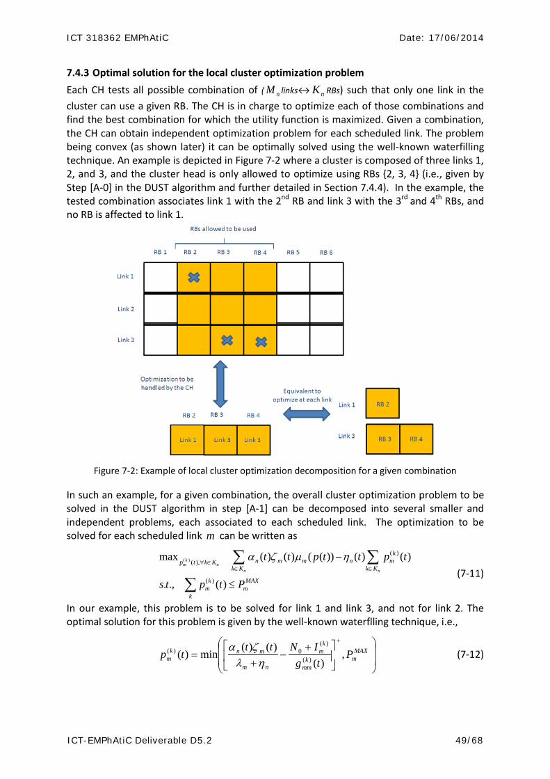
ICT 318362 EMPhAtiC Date: 17/06/2014
ICT-EMPhAtiC Deliverable D5.2 49/68
7.4.3 Optimal solution for the local cluster optimization problem Each CH tests all possible combination of ( nM links↔ nK RBs) such that only one link in the cluster can use a given RB. The CH is in charge to optimize each of those combinations and find the best combination for which the utility function is maximized. Given a combination, the CH can obtain independent optimization problem for each scheduled link. The problem being convex (as shown later) it can be optimally solved using the well-known waterfilling technique. An example is depicted in Figure 7-2 where a cluster is composed of three links 1, 2, and 3, and the cluster head is only allowed to optimize using RBs {2, 3, 4} (i.e., given by Step [A-0] in the DUST algorithm and further detailed in Section 7.4.4). In the example, the tested combination associates link 1 with the 2nd RB and link 3 with the 3rd and 4th RBs, and no RB is affected to link 1.
Figure 7-2: Example of local cluster optimization decomposition for a given combination
In such an example, for a given combination, the overall cluster optimization problem to be solved in the DUST algorithm in step [A-1] can be decomposed into several smaller and independent problems, each associated to each scheduled link. The optimization to be solved for each scheduled link m can be written as
( )( )
( ),
( )
max ( ) ( ) ( ( )) ( ) ( )
. ., ( )
km n
n n
kn m m n mp t k K
k K k K
k MAXm m
k
t t p t t p t
s t p t P
α ζ µ η∀ ∈
∈ ∈
−
≤
∑ ∑
∑ ( 7-11)
In our example, this problem is to be solved for link 1 and link 3, and not for link 2. The optimal solution for this problem is given by the well-known waterflling technique, i.e.,
+−
+=
+
MAXmk
mm
km
nm
mnkm P
tgINtt
tp ,)(
)()(min)( )(
)(0)(
ηλζα
( 7-12)

ICT 318362 EMPhAtiC Date: 17/06/2014
ICT-EMPhAtiC Deliverable D5.2 50/68
To solve for this equation, one need to know first mλ which represents the Lagrangian relative to the maximum power constraint MAX
mP . Linearly decreasing in terms of mλ , this can be easily solved using for example the bisection method such that
MAXmk
MAXmk
mm
km
nm
mn PPtgINtt
=
+−
+∑+
,)(
)()(min )(
)(0
ηλζα
( 7-13)
7.4.4 Algorithm to adapt the selection of the resource blocks set In the clusterized ad-hoc scenario depicted in Figure 7-3 the 3 sets of RBs have been allocated to the 9 clusters such that the spatial reuse is maximized.
Figure 7-3: Example of 9 clusters with an elected CH each (i.e., red larger mobile); each
cluster is allowed to use one of the three sets of RBs (i.e., (1, 2), (3, 4), (5, 6))
In the envisioned scenario network where the inter-cluster communication is very limited through a dedicated channel, it may not be possible to add a communication protocol (along with the cumulated queue information exchange) to converge to a similar situation depicted in Figure 7-3. On the opposite side, it is not good to randomly associate the RBs sets to the clusters and remain with the same allocation all the time. This could lead to too many nearby interfering clusters. To avoid such inefficiency, it is possible to make the system more intelligent and dynamic by exploring other sets and learning from the past. The idea is to randomly explore other sets, while adjusting in time the new searches by giving more priority to the better possible sets. To do so, we use the following approach. Denote by { },....,, 321
nnn ttt the time instances when the thn cluster decides to test a new RBs set. We assume that each time in the set { },....,, 321
nnn ttt belongs to the larger time instances where
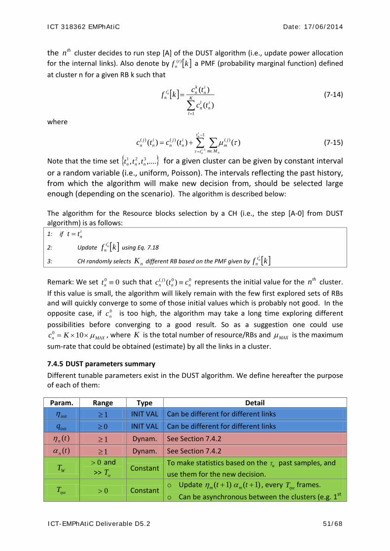
ICT 318362 EMPhAtiC Date: 17/06/2014
ICT-EMPhAtiC Deliverable D5.2 51/68
the thn cluster decides to run step [A] of the DUST algorithm (i.e., update power allocation for the internal links). Also denote by [ ]kf t
n)( a PMF (probability marginal function) defined
at cluster n for a given RB k such that
[ ]∑=
= K
l
in
ln
in
knt
n
tc
tckfin
1)(
)( ( 7-14)
where
∑ ∑−
= ∈−
+=1
)()()(
1
)()()(in
in n
t
t Mm
jm
in
jn
in
jn tctc
τ
τµ ( 7-15)
Note that the time set { },....,, 321nnn ttt for a given cluster can be given by constant interval
or a random variable (i.e., uniform, Poisson). The intervals reflecting the past history, from which the algorithm will make new decision from, should be selected large enough (depending on the scenario). The algorithm is described below: The algorithm for the Resource blocks selection by a CH (i.e., the step [A-0] from DUST algorithm) is as follows: 1: if i
ntt =
2: Update [ ]kfint
n using Eq. 7.18
3: CH randomly selects nK different RB based on the PMF given by [ ]kfint
n
Remark: We set 00 ≡nt such that 00)( )( nnj
n ctc ≡ represents the initial value for the thn cluster. If this value is small, the algorithm will likely remain with the few first explored sets of RBs and will quickly converge to some of those initial values which is probably not good. In the opposite case, if 0
nc is too high, the algorithm may take a long time exploring different possibilities before converging to a good result. So as a suggestion one could use
MAXn Kc µ××= 100 , where K is the total number of resource/RBs and MAXµ is the maximum sum-rate that could be obtained (estimate) by all the links in a cluster.
7.4.5 DUST parameters summary Different tunable parameters exist in the DUST algorithm. We define hereafter the purpose of each of them:
Param. Range Type Detail
initη 1≥ INIT VAL Can be different for different links
initq 0≥ INIT VAL Can be different for different links )(tnη 1≥ Dynam. See Section 7.4.2 )(tnα 1≥ Dynam. See Section 7.4.2
WT 0> and
>> αT Constant To make statistics based on the WT past samples, and use them for the new decision.
ηαT 0> Constant o Update )1( +tmη )1( +tmα , every ηαT frames. o Can be asynchronous between the clusters (e.g. 1st
ICT 318362 EMPhAtiC Date: 17/06/2014
ICT-EMPhAtiC Deliverable D5.2 52/68
Cluster update at [2, 2+ ηαT , 2+2 ηαT , 2+3 ηαT n…], and 5th cluster update at [9, 9+ ηαT , 9+2 ηαT , 9+3
ηαT ,…] o Can be different value for different clusters
1ε [ ]1,0 Constant
This randomly forces the cluster which does not succeed to fulfill his required throughput (i.e., high internal link queues) to back-off transmitting. To do so, α is decreased when 1() ε<rand . This is to ‘heuristically’ cope with two adjacent clusters always competing and never succeeding to transmit anything.
UPη >1 Constant A multiplicative factor to increase η DOWNη [0,1) Constant A multiplicative factor to decrease η HIGHη 0> Constant Value of η assumed to be high
ADDα 0> Constant A constant to increase α
DEACRα 0> Constant A constant to decrease α
DOWNα [0,1) Constant A multiplicative factor to decrease α
Table 7-1: DUST parameters summary
7.5 Numerical experiments
7.5.1 Simulations objectives The main objectives of the current simulations are the following: Compare the performance with perfect modulation (i.e., no adjacent interference),
with OFDM, and with FBMC. Higher adjacent V parameters simply means higher total cross interference, thus it is expected that algorithms should have better behavior with FBMC.
Effect of different input rates (i.e., low / high traffic requirements).
Effect of random cluster scheduling compared to exact same round-robin scheduling (we assume that only one cluster is waken-up for optimizing its resources and for broadcasting at a time)
Effect of different update time interval ηαT to update the dynamic parameters nη
and nα .
7.5.2 Detailed settings We now evaluate the DUST algorithm using the scenario described in Section 2.2.3. The parameters are the following:
• Cluster definition
o Each cluster is represented by the square area with side length C=300m
o Nb. Clusters: 9 (i.e., 3x3)
o Nb. Links per cluster: 3

ICT 318362 EMPhAtiC Date: 17/06/2014
ICT-EMPhAtiC Deliverable D5.2 53/68
• Nodes’ location (TX/RX pairs) :
o Transmitters are randomly located with their affiliated cluster
o The associated receiver is located using ),( rθ from the TX, where the angular distribution is uniformly distributed over [0, 2π) and the distance is also uniformly distributed over (0, C/4]
• Traffic load
o All users have a constant input bit rate, i.e., mm ata =)( bits t∀ .
The reference traffic, named (x1), is a constant bit traffic where ma for each link is around 5 to 10 bits/second. Those rates were
obtained by transmitting with maximum power and using 2 RBs from each link and turning-off the others using the same RBs set, then dividing by 6 assuming that 2 clusters are competing for the same set of 2 RBs with 3 links each.
• RB allocation constraint:
o One subcarrier: 15 kHz
o RB minimum concatenated subcarriers: 12
o RB equivalent bandwidth: 0.18 MHz (12*15kHz)
o In each cluster only 1 link can be scheduled on a given RB.
o Total available RB for allocation: 6
• We enforce a pre-allocation of 2 RBs out of the available 6 RBs to each cluster as depicted in Figure 7-3, i.e.,
Cluster 1: {1, 2} Cluster 2: {3, 4} Cluster 3: {5, 6}
Cluster 4: {5, 6} Cluster 5: {1, 2} Cluster 6: {3, 4}
Cluster 7: {3, 4} Cluster 8: {5, 6} Cluster 9: {1, 2}
The purpose of such mapping is to have the best space reuse to avoid too many adjacent clusters using the same resource. However, interference still exists that cannot be avoided due to the limited number of RBs and small areas. Using the notation used earlier (see DUST algorithm), we have for example { }2,15 =K , i.e., the set of RBs allocated to 5th cluster is composed of RB 1 and 2.
• Channel characteristics:
o Path-loss model: ITU-R P.1411-4 [10]
o Shadowing: 9 dB standard deviation
• Transmit power max: 30 dBm (mobile characteristics for generality)
• Noise level: -174 dBm/Hz
• The adjacent interference coefficient ν has been computed using the interference values given in Eq. 4.6-4.7 of reference [25], computed per subcarrier. We recall that the v has been derived by assuming that the clusters are asynchronous with a time

ICT 318362 EMPhAtiC Date: 17/06/2014
ICT-EMPhAtiC Deliverable D5.2 54/68
delay which is uniform over the duration of the OFDM symbol. We applied those values to our MAC/Phy setting, i.e.,
o 1 RB contains 12 subcarriers o 6 RBs available within the 1.4 MHz bandwidth
Based on this setting we obtain the following interference vector between RB, Based on this setting we obtain the following interference vector between RB, which has been calculated by evaluating the interference of each subcarrier of a RB and then adding together the contributions of all the subcarriers inside a RB. Notice that when an asynchronous user is transmitting over the same RB of an interfered link, the interference is higher than one. This is due to the fact that a given subcarrier sees and interference of 1 due to the same subcarrier of the interfering signal plus the interference generated by the non-synchronization of the adjacent interfering subcarriers inside the same RB.
Modulation type Vector of interference coefficient
[…, v(-2), v(-1), v(0), v(1), v(2), v(3), …] Perfect [0, 1, 0] OFDM [0.0201, 1.2324, 0.0201 ] FBMC [0.0073, 1.1615, 0.0073]
Table 7-2: Specific interference coeffcients
Note that v )0( is the direct interference when two links use the same RB, v )1(− is the adjacent interference from the left-hand side RB whereas v )1( is the adjacent interference from the right-hand side RB. Looking at the values in the table, one can observe that we assume here a symmetric adjacent interference (i.e., left/right). The constant values used for the DUST parameters described in Table 7-1 is summarized in the table below:
Param. Value Compared with
initη 3*rand()
initq 0
WT 1000
ηαT 100 Compared with: {2, 50, 500}
1ε 0.4
UPη 1.1 DOWNη 0.9 HIGHη 1000
ADDα 0.5
DEACRα 1
DOWNα 0.75
Table 7-3: Specific parameter values used for the simulations

ICT 318362 EMPhAtiC Date: 17/06/2014
ICT-EMPhAtiC Deliverable D5.2 55/68
7.5.3 Numerical results In the following numerical experiments section, two metrics are used to analyze the DUST algorithm performance in different settings.
Theoretical output over input ratio:
∑
∑
+−=
+−==MAX
MAX
MAX
MAX
T
Tm
T
Tm
amMetric
110
1101
5
5
)(
)()(
τ
τ
τ
τµ
Average transmitted power: ∑+−=
=MAX
MAX
T
TmpmMetric110
525
)(10
1)(τ
τ
where we use a window averaging over the last samples with 5102×=MAXT samples.
Note that the averaging is starting late, i.e., from 510=t , in order to discard possible initial transient phase of the algorithm before its convergence. For each of the two metrics, the x-axis represents the id m for each of the 27 links (i.e., 9 clusters with 3 links each).
In Figure 7-4 )(1 mMetric is shown for three sub-plots related to different modulation (i.e., perfect modulation, OFDM, and FBMC). Each sub-plot contains 4 curves representing different traffic loads. Based on the reference traffic load defined earlier, called (x1), the other three traffics are defined as larger traffic load given by the corresponding multiplicative value (i.e., x1.5, x1.75, x2). Let us clarify the way to read the figure. A positive y-axis means that the average theoretical throughput is larger than the average input bits to the data buffer. A negative y-axis means that the average output is lower than the average input, meaning that the data buffer is not well stabilized and increases.
Looking at the low reference traffic load (i.e., x1), it is easy to observe that in any of the three modulation type, the metric is positive (about 10-15%). In an optimal solution, one would have expected something closer to 0% and positive. However, this DUST algorithm is a heuristic algorithm and most importantly not a centralized algorithm. Thus, 10 to 15% higher theoretical throughput can be assumed as acceptable. Now increasing the load, one can observe that the metrics starts decreasing. In particular for the OFDM and FBMC case, with Load x2 (i.e., the maximum load tested), the ratio is generally negative, whereas the ratio for the Perfect Modulation remains in general positive. This shows that with load requirement closer to the network capacity and the additional imperfection of those modulations, the DUST algorithm cannot achieve the required throughput. One can however observe that the performance of the FBMC is better than the one for OFDM. This is of course expected since the adjacent interference as well as the direct interference is higher for OFDM compared to FBMC (see Table 7-2).
510

ICT 318362 EMPhAtiC Date: 17/06/2014
ICT-EMPhAtiC Deliverable D5.2 56/68
Figure 7-4: Output over input ratio ( )(1 mMetric ) comparison for different modulations and
different traffic loads
Figure 7-5 presents the associated average transmit power (i.e., )(2 mMetric ) to the performance presented in Figure 7-4. It is easy to observe that with higher traffic load the power consumption becomes higher in general. Note that 30dBm (i.e., 1W) is the maximum transmit power at each link. For the case of Load x2, the OFDM and FBMC modulation exhibits close to maximum transmission power. In parallel, we have seen through Figure 7-4, that the corresponding )(1 mMetric were negative. This means that they are often competing with maximum transmission power to compensate for always higher inter-cluster interferences but fail to reach their required throughput rate. However, we can note that the negative values in Figure 7-4 is not going below -20%, which is not acceptable yet not completely bad (i.e., we do not get unstable solutions with some of the links having really bad solution).
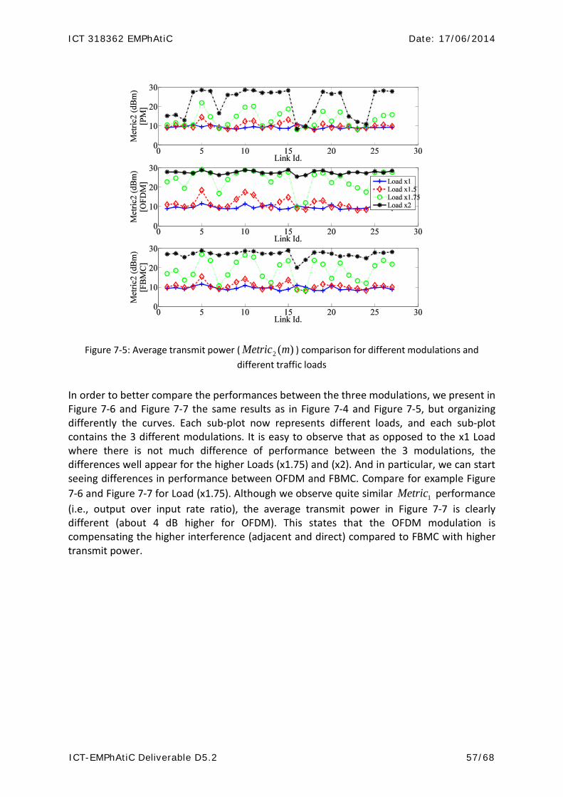
ICT 318362 EMPhAtiC Date: 17/06/2014
ICT-EMPhAtiC Deliverable D5.2 57/68
Figure 7-5: Average transmit power ( )(2 mMetric ) comparison for different modulations and
different traffic loads
In order to better compare the performances between the three modulations, we present in Figure 7-6 and Figure 7-7 the same results as in Figure 7-4 and Figure 7-5, but organizing differently the curves. Each sub-plot now represents different loads, and each sub-plot contains the 3 different modulations. It is easy to observe that as opposed to the x1 Load where there is not much difference of performance between the 3 modulations, the differences well appear for the higher Loads (x1.75) and (x2). And in particular, we can start seeing differences in performance between OFDM and FBMC. Compare for example Figure 7-6 and Figure 7-7 for Load (x1.75). Although we observe quite similar 1Metric performance (i.e., output over input rate ratio), the average transmit power in Figure 7-7 is clearly different (about 4 dB higher for OFDM). This states that the OFDM modulation is compensating the higher interference (adjacent and direct) compared to FBMC with higher transmit power.
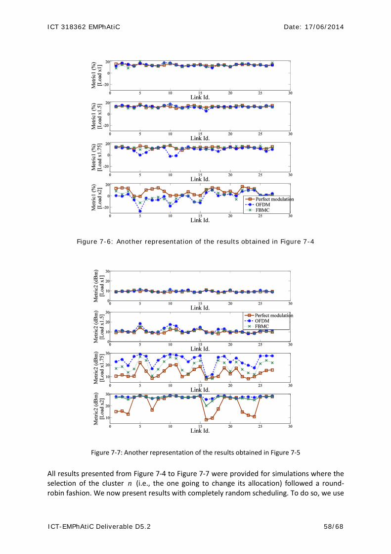
ICT 318362 EMPhAtiC Date: 17/06/2014
ICT-EMPhAtiC Deliverable D5.2 58/68
Figure 7-6: Another representation of the results obtained in Figure 7-4
Figure 7-7: Another representation of the results obtained in Figure 7-5
All results presented from Figure 7-4 to Figure 7-7 were provided for simulations where the selection of the cluster n (i.e., the one going to change its allocation) followed a round-robin fashion. We now present results with completely random scheduling. To do so, we use
ICT 318362 EMPhAtiC Date: 17/06/2014
ICT-EMPhAtiC Deliverable D5.2 59/68
Load x1.5 and x1.75, and compare the performances with the one obtained previously with the round-robin approach. Figure 7-8 and Figure 7-9 correspond to Load x1.5 whereas Figure 7-10 and Figure 7-11 correspond to Load x1.75. It is easy to observe that the random scheduling approach yields quite similar performance to the round-robin approach. However, looking at Figure 7-10 and Figure 7-11, a slight advantage for the randomized scheduling can be noticed. It is difficult to comment this result in general. Intuitively speaking, because each cluster have completely random {links location, traffic, and channels}, using random scheduling of the cluster on the 9 block grid seems obviously better than a strict round-robin fashion. Note that in the literature the iterative waterfilling algorithms are known to work for completely asynchronous nodes (although the achieved rate quality and convergence is not necessarily guaranteed for high inter-cell interferences).
Figure 7-8: Output over input ratio ( )(1 mMetric ) comparison using traffic load (x1.5) for different
modulations between round-robin and random cluster selection

ICT 318362 EMPhAtiC Date: 17/06/2014
ICT-EMPhAtiC Deliverable D5.2 60/68
Figure 7-9: Average transmit power ( )(2 mMetric ) comparison using traffic load (x1.5) for different
modulations between round-robin and random cluster selection
Figure 7-10: Output over input ratio ( )(1 mMetric ) comparison using traffic load x1.75 for
different modulations between round-robin and random cluster selection

ICT 318362 EMPhAtiC Date: 17/06/2014
ICT-EMPhAtiC Deliverable D5.2 61/68
Figure 7-11: Average transmit power ( )(2 mMetric ) comparison using traffic load (x1.75)
for different modulations between round-robin and random cluster selection
Finally, we now test the effect of the update time interval ηαT to update the dynamic
parameters nη and nα . Previous simulations have been performed using 100=ηαT . Now, three additional time intervals { }500,50,2=ηαT have been tested for comparison Figure 7-12 and Figure 7-13 provides the performance comparison for the four time intervals, for the three modulations as usual. It is easy to observe that 2=ηαT yields quite bad results
since )(1 mMetric is often negative (e.g., -100%) and in addition yields large )(2 mMetric . Comparing the three other cases, i.e., { }500,100,50=ηαT , we can observe that for
500=ηαT )(1 mMetric is positive but is in general higher than for { }100,50=ηαT . As stated earlier, from an optimal point of view one would expect a positive but close to zero percentage value such that the energy is minimized. Finally, comparing { }100,50=ηαT ,
although )(1 mMetric is quite similar, we can observe from )(2 mMetric a slight advantage for 50=ηαT which uses less power. Thus, comparing the 4 tested update time intervals, we can conclude that it is better for this tested scenario to use 50=ηαT . But of course we cannot generalize since the choice of ηαT will depend on different properties of the scenario like the channels, the traffics, the level of interfering clusters, etc. It is therefore hard to provide a theoretical way to choose that constant parameter. However, from an intuitive point-of-view we would suggest to set it few times larger than the number of clusters.
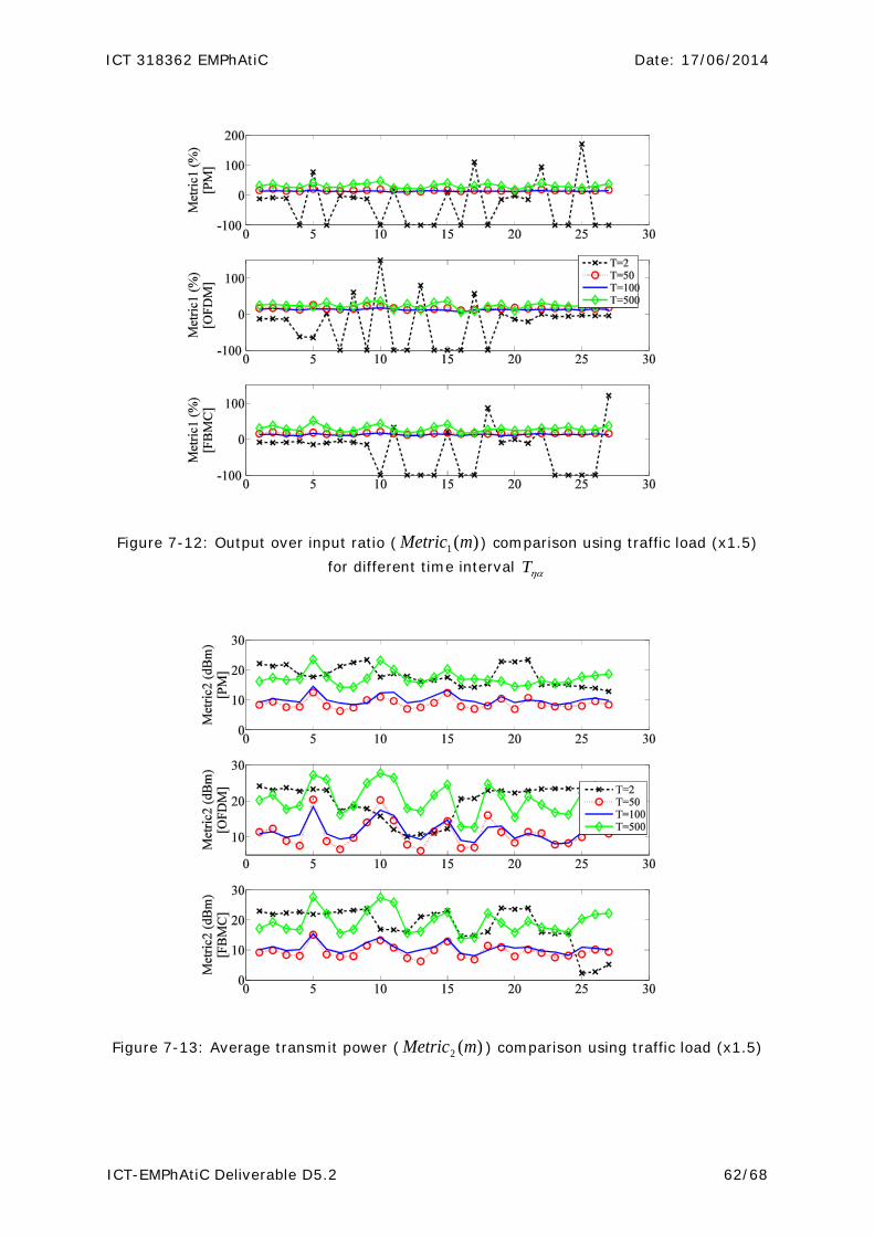
ICT 318362 EMPhAtiC Date: 17/06/2014
ICT-EMPhAtiC Deliverable D5.2 62/68
Figure 7-12: Output over input ratio ( )(1 mMetric ) comparison using traffic load (x1.5)
for different time interval ηαT
Figure 7-13: Average transmit power ( )(2 mMetric ) comparison using traffic load (x1.5)
ICT 318362 EMPhAtiC Date: 17/06/2014
ICT-EMPhAtiC Deliverable D5.2 63/68
7.6 Miscellaneous discussions
The main characteristics of the DUST algorithm can be summarized as follows: Minimize the transmission energy while keeping the data buffer stable for each link
in a cluster. Distributed approach with limited exchanges:
o Each cluster only knows the total queue size of the other clusters o Total queue size single value is transmitted on a dedicated control channel o Asynchronous: a cluster decides to update its optimized resource when it
wants (the random scheduling and the round-robin approaches were tested)
Possible ways for improvements: Choice of the virtual queue nζ mathematical design: The virtual weighting queue is
based on the relative ratio between each node’s buffer size compared to the total queue size of the network (at least received from decoded broadcasting). Thus, this queue design prioritizes the users with higher traffic (thus no fairness). Imagine two interfering users with the same channel quality but the first user has 1Mbit/s of input bits to its data buffer whereas the second user has only 10kb/s. In such a case user 2 will only be scheduled when its queue size is as large as or larger than for user 1. This means that user 2 will experience high latency.
Further interesting investigations: Choice of WT and ηαT : Their individual and combined effects on the algorithm
performance should be further investigated. Their values should certainly be customized to the scenario variability (i.e., traffic, and channel). Moreover, it could be envisioned to vary those parameters in time (within a longer time frame).
Update of )(tmα and )(tmη along time: Their individual and combined effects on the algorithm performance should be further investigated. In particular, those updates have been designed in a heuristic way and may probably be improved.
In the two scheduling approaches (i.e., random or round-robin), we assume that at given simulation time only one cluster optimizes, changes its allocation, and broadcasts the new allocation. We also assume that each of the cluster receive all broadcasts without error. Now, it is possible to imagine that many clusters decide to change at the same time (more probable in practical asynchronous network). Thus, broadcast collisions may appear in which case a local modification may not be know by others, at least until the next successful broadcast.
o Although not tested, it is believed that the DUST algorithm should be quite robust for such small losses, if one can assume that the percentages of broadcast losses are kept low. This is because the only information exchanged is the local total queue size which constantly changes in time.
o It can be envisioned to run the algorithm where each broadcast is only received by only the nearby clusters, i.e., broadcasts received with SINR larger than some threshold. Such restriction, in the case of only one scheduled cluster at a time, may not be a problem for the algorithm. This is because low SNR shows that the CH transmitter may be far enough such that even its data transmission using the same RB may not be a problem (i.e., spatial frequency reuse). However, in the case where multiple clusters can

ICT 318362 EMPhAtiC Date: 17/06/2014
ICT-EMPhAtiC Deliverable D5.2 64/68
broadcast at the same time, the low SINR cannot be simply interpreted as far away cluster, which will necessarily impact the data transmission as well.
The only information which is exchanged is the total buffer size of the local cluster. In practice this information should be quantized. However, it is believed that the quantification would have no impact at all on the performance, and will be easily averaged in time, thanks to the nature of the value (i.e., large integer).
As for the impact of the OFDM vs FBMC on the RRM performance, we have seen that they are more pronounced when the traffic requirement increases. This is because higher throughput necessarily requires more transmit power, and since OFDM exhibits larger interference than FBMC, the inter-cluster interferences become more pronounced and an additional increase in power is required to compensate (to a certain limit since what count is the SINR and not only the received power). And as expected the Perfect Modulation (as it is called) outperforms FBMC which outperforms OFDM.
ICT 318362 EMPhAtiC Date: 17/06/2014
ICT-EMPhAtiC Deliverable D5.2 65/68
8. Conclusions
In this report a thorough study of RRM algorithms for PMR communications has been provided, while different solutions for optimizing RRM have been proposed and evaluated on top of the FBMC scheme. More specifically, PMR scenarios for synchronized and unsynchronized communications have been defined, referring to well-planned and randomly deployed networks. The recent advances of PMR communications have been listed, including the enabling of direct communications where the intermediate transmissions to the BS are avoided. The most important open challenges for this type of communication have been summarized, and a resource request/allocation scheme for the direct operation has been proposed. For the defined scenarios, a series of RRM schemes has been proposed and evaluated on top of FBMC scheme towards providing scheduling priority to PMR traffic and optimizing the resource allocation procedure. Results revealed the superiority of FBMC against CP-based solutions such as the OFDM, especially in unsynchronized and centrally controlled scenarios.

ICT 318362 EMPhAtiC Date: 17/06/2014
ICT-EMPhAtiC Deliverable D5.2 66/68
9. References [1] X. Lin, J. G. Andrews, A. Ghosh, and R. Ratasuk, “An Overview on 3GPP Device-To-
Device Proximity Services,” arXiv preprint arXiv:1310.0116, 2013. [2] F. Baccelli, M. Klein, M. Lebourges, and S. Zuyev, “Stochastic geometry and
architecture of communication networks,” J. Telecommunication Systems, vol. 7, pp. 209–227, 1997.
[3] X. Lin, J. G. Andrews, A. Ghosh, and R. Ratasuk, “An Overview on 3GPP Device-To-Device Proximity Services,” arXiv preprint arXiv:1310.0116, 2013.
[4] 3GPP TS 36.300, v9.9.0, Rel.9, “Evolved Universal Terrestrial Radio Access (E-UTRA) and Evolved Universal Terrestrial Radio Access Network (E-UTRAN),” overall description, Jan. 2013.
[5] K. Doppler, M. Rinne, C. Wijting, C.B. Ribeiro, K. Hugl, “Device-to-device communication as an underlay to LTE-advanced networks,” IEEE Communications Magazine, vol.47, no.12, pp.42,49, Dec. 2009.
[6] 3GPP TS36.321 v9.6.0, Rel.9, “Evolved Universal Terrestrial Radio Access (E-UTRA), Medium Access Control (MAC) protocol specification”, Mar. 2012.
[7] Deliverable D6.1, “Cooperative communications and synchronization”, FP7 Emphatic project.
[8] Y. Medjahdi, M. Terre, D. Le Ruyet, D. Roviras, J. A. Nossek, and L. Baltar, “Inter-cell Interference Analysis for OFDM / FBMC Systems,” in Proc. Of 10th IEEE Signal Processing Workshop (SPAWC 2009), Perugia, Italy, June 2009.
[9] W. Yu, W. Rhee, S. Boyd, and J. M. Cioffi, “ Iterative waterfilling for Gaussian vector multiple access channels,” IEEE Trans. Inf. Theory, vol. 50, pp. 145–152, Jan. 2004.
[10] ITU-R P.1411-4, Propagation data and prediction methods for the planning of short-range outdoor radiocommunication systems and radio local area networks in the frequency range 300 MHz to 100 GHz.
[11] K. Huang and J. G. Andrews ,’’ An analytical framework for multicell cooperation via stochastic geometry and large deviations‘’ IEEE Trans. On, Information Theory, vol. 59, no. 4, pp 2501-2516, April 2013.
[12] I. Kim, I.-S Park, and Y. H. Lee,’’ Use of linear programming for dynamic subcarrier and bit allocation in multiuser OFDM‘’ IEEE Trans. On, Vehicular Technology, vol. 55, no. 4, pp 1195-1207, July 2006.
[13] W. Rhee and J. Cioffi,”Increase in capacity of multiuser OFDM system using dynamic subchannel allocation” in IEEE 51th Vehic. Techn. Conference Proceedings, vol.2, 2000, pp 1085-1089
[14] L. Vijayandran, S. S. Byun, G. E. Øien, T. Ekman, “Increasing sum-rate in large scale cognitive radio networks by centralized power and spectrum allocation,” Eurasip Journal on Wireless Communications and Networking, 2012:362, Dec. 12.
[15] L. Qian, Y. J. Zhang, and M. Chiang, “Distributed nonconvex power control using Gibbs Sampling,”IEEE Transactions on Communications, vol. 60, no. 12, pp. 3886-3898, Dec. 2012.
[16] J. Papandriopoulos and J. S. Evans, “Low-complexity distributed algorithms for spectrum balancing in multi-user DSL networks,” In Proc. IEEE ICC, pp. 3270–3275, Istanbul, Turkey, June 2006.
[17] D. Schmidt et al., “Distributed resource allocations schemes,” IEEE Signal Processing Magazine, Sep. 2009.

ICT 318362 EMPhAtiC Date: 17/06/2014
ICT-EMPhAtiC Deliverable D5.2 67/68
[18] W. Yu, G.Ginis, and H. M. Cioffi, “Distributed multiuser power control for digital subscriber lines,” IEEE J. Select. Areas Commun., vol. 2, no. 5, June 2002.
[19] M. Pischella, D. Le Ruyet, Y. Medjahdi, “Sum rate maximization in asynchronous ad hoc networks: comparison of multi-carrier modulations,” In Proc. IEEE ISWCS, pp. 1-5, Ilmenau, Germany, Aug. 2013.
[20] J. Huang, R. A. Berry, and M. L. Honig, “Distributed interference compensation for wireless networks,” IEEE J. Select. Areas Commun., vol. 24, no. 5, pp. 1074–1084, May 2006.
[21] J. Mo and J. Walrand, “Fair end-to-end window-based congestion control,” IEEE/ACM Transactions on Networking, vol. 8, no. 5, pp. 556–567, Oct. 2000.
[22] Chiang M, Tan C, Palomar D, Neill DO, Julian D: Power Control By Geometric Programming. IEEE Trans. Wireless Commun. 2007, 6(7):2640–2651.
[23] L. Georgiadis, M. J. Neely, and L. Tassiulas. Resource allocation and cross-layer control in wireless networks. Foundations and Trends in Networking, 1(1):1–144, 2006.
[24] M. J. Neely, “Energy optimal control for time-varying wireless networks,” IEEE Trans. Information Theory, vol. 52, no. 7, pp. 2915–2934, Jul. 2006.
[25] Deliverable D5.1, “Study of the advantages of FBMC in RRM for PMR”, FP7 Emphatic project.
ICT 318362 EMPhAtiC Date: 17/06/2014
ICT-EMPhAtiC Deliverable D5.2 68/68
Glossary and Definitions
Acronym Meaning 3GPP 3rd Generation Partnership Project BS Base Station CP Cyclic Prefix CH Cluster Head DMO Direct Mode Operation FBMC Filter Bank Multicarrier HH Hand Held MAC Medium access control MCS Modulation and coding scheme MS Mobile Station OFDM Orthogonal Frequency Division Multiplexing PHY Physical layer PMR Professional Mobile Radio ProSe Proximity Services PF Proportional Fair PUCCH Physical Uplink Control Channel PUSCH Physical Uplink Shared Channel RRM Radio Resource Management RS Relay Station RB Resource Block RA Resource Allocation SC-FDMA Single Carrier – Frequency Division Multiple Access TDMA Time division multiple access