Enhanced MPPT Controllers for Smart Grid Applications
95
Rochester Institute of Technology Rochester Institute of Technology RIT Scholar Works RIT Scholar Works Theses 4-2019 Enhanced MPPT Controllers for Smart Grid Applications Enhanced MPPT Controllers for Smart Grid Applications Mohamed Khallaf [email protected] Follow this and additional works at: https://scholarworks.rit.edu/theses Recommended Citation Recommended Citation Khallaf, Mohamed, "Enhanced MPPT Controllers for Smart Grid Applications" (2019). Thesis. Rochester Institute of Technology. Accessed from This Thesis is brought to you for free and open access by RIT Scholar Works. It has been accepted for inclusion in Theses by an authorized administrator of RIT Scholar Works. For more information, please contact [email protected].
Transcript of Enhanced MPPT Controllers for Smart Grid Applications
Rochester Institute of Technology Rochester Institute of Technology
RIT Scholar Works RIT Scholar Works
Theses
4-2019
Enhanced MPPT Controllers for Smart Grid Applications Enhanced MPPT Controllers for Smart Grid Applications
Mohamed Khallaf [email protected]
Follow this and additional works at: https://scholarworks.rit.edu/theses
Recommended Citation Recommended Citation Khallaf, Mohamed, "Enhanced MPPT Controllers for Smart Grid Applications" (2019). Thesis. Rochester Institute of Technology. Accessed from
This Thesis is brought to you for free and open access by RIT Scholar Works. It has been accepted for inclusion in Theses by an authorized administrator of RIT Scholar Works. For more information, please contact [email protected].

i
RIT
Enhanced MPPT Controllers for Smart Grid
Applications
by
Mohamed Khallaf
A Thesis Submitted in Partial Fulfillment of the
Requirements for the Degree of Master of Science in Electrical Engineering
Department of Electrical Engineering and Computing Sciences
Rochester Institute of Technology, Dubai UAE
April 2019

ii
Enhanced MPPT Controllers for Smart Grid Applications
by
Mohamed Khallaf,
A Thesis Submitted in Partial Fulfillment of the Requirements
for the Degree of Master of Science in Electrical Engineering
Department of Electrical Engineering and Computing Sciences
Approved By:
_____________________________________________Date:______________
Dr. Abdulla Ismail
Thesis Advisor –Department of Electrical Engineering
_____________________________________________Date:______________
Dr. Yousef Al Assaf
Committee Member –Department of Electrical Engineering
_____________________________________________Date:______________
Dr. Mohamed Samaha
Committee Member –Department of Mechanical Engineering

iii
Acknowledgements I would like to express the deepest appreciation to Dr. Abdulla Ismail, my thesis
advisor, for his tremendous guidance and encouragement. Dr. Abdulla has been
instrumental for the success of my thesis and I am honored to have had him as my
advisor.
Besides my advisor, I would like to thank the rest of my thesis committee: Dr. Yousef
Al Assaf, President of RIT Dubai and Dr. Mohamed Samaha, Professor of
Mechanical Engineering at RIT Dubai, on their insightful comments which allowed
me to widen my research from various perspectives.
Last but not least, I would like to express my gratitude to my family: my parents and
sisters for their endless support and motivation throughout this journey. Without them
this thesis would not have been possible.

iv
Dedicated to my family.
v
Table of Contents Table of Contents ......................................................................................................... vList of Figures ............................................................................................................ viiList of Tables ............................................................................................................. viiiList of Abbreviations .................................................................................................. ixList of Publications ...................................................................................................... xAbstract….. .................................................................................................................. 1Chapter 1 Introduction ............................................................................................. 31.1Motivation.................................................................................................................................31.2ResearchObjectives..............................................................................................................41.3ThesisOrganization...............................................................................................................4
Chapter 2 Problem Background .............................................................................. 52.1Introduction..............................................................................................................................52.2IntroductiontoSmartGrids...............................................................................................52.2.1ChallengesofaSmartGrid.......................................................................................10
2.3RenewableEnergyResources.........................................................................................112.3.1PVpenetratedpowersystem.................................................................................112.3.2PVPenetratedPowerSystemChallengingIssues.........................................132.3.3MaximumPowerPointTracking(MPPT).........................................................152.3.4EffectofPartialShading............................................................................................16
Chapter 3 MPPT Controllers ................................................................................. 193.1Perturb&ObserveAlgorithm.........................................................................................193.1.1Introduction...................................................................................................................193.1.2MethodofOperation..................................................................................................203.1.3AdvantagesanddisadvantagesofP&Omethod.............................................23
3.2MPPTusingIncrementalConductance(INC)..........................................................243.2.1Introduction...................................................................................................................243.2.2MethodofOperation..................................................................................................263.2.3AdvantagesandDisadvantagesofINC...............................................................293.2.4INCCoupledwithIntegralRegulator(IR).........................................................29
3.3MPPTUsingFuzzyLogicController.............................................................................313.3.1IntroductiontoFuzzyLogic....................................................................................313.3.2FuzzySetsandMembershipFunctions..............................................................313.3.3FuzzyRulesandReasoning.....................................................................................343.3.4FuzzyLogicController...............................................................................................363.3.5MethodofOperation..................................................................................................373.3.6AdvantagesandDisadvantagesofFuzzyLogic..............................................39
Chapter 4 Design & Analysis ................................................................................. 414.1Introduction............................................................................................................................414.2SystemArchitecture............................................................................................................424.2.1PhotovoltaicModule...................................................................................................444.2.2MPPT.................................................................................................................................454.2.3DC-DCConverter..........................................................................................................49
4.3EffectofTemperatureandIrradianceonthePVOutputPower......................51Chapter 5 Discussion and Results .......................................................................... 555.1Introduction............................................................................................................................555.2Perturb&ObserveAlgorithmResults.........................................................................575.2.1ScenarioOne:ConstantIrradianceandTemperature.................................57
vi
5.2.2ScenarioTwo:VaryingIrradianceandTemperature..................................605.3IncrementalConductance+IntegralRegulator.......................................................645.3.1ScenarioOne:ConstantIrradianceandTemperature.................................645.3.2ScenarioTwo:VaryingIrradianceandTemperature..................................67
5.4FuzzyLogicController.......................................................................................................715.4.1ScenarioOne:ConstantIrradianceandTemperature.................................715.4.2ScenarioTwo:VaryingIrradianceandTemperature..................................73
Chapter 6 Conclusion ............................................................................................. 766.1ResearchObjectives............................................................................................................766.2SummaryofResearchResults........................................................................................776.2.1ResultsofConstantConditions–Scenario1...................................................776.2.2ResultsofVaryingConditions–Scenario2......................................................776.2.3ComparisonbetweenControllers’Characteristics.......................................79
6.3RecommendationsforFutureWork............................................................................80References:… ............................................................................................................. 81Appendix A: ............................................................................................................... 84P&OMATLABCode:....................................................................................................................84
vii
List of Figures Figure 2.1 Smart Grid Components...............................................................................................7Figure 2.2 PV System Components.............................................................................................12Figure 2.3 PV System Process.......................................................................................................14Figure2.4VoltageVersusCurrentofMPPTGraph..........................................................16Figure 2.5 Comparison between No and Partial Shading.....................................................17Figure 2.6 Partial Shading Conditions Power Curve..............................................................18Figure 3.1 Power Versus Voltage Curve Showing P&O’s Operation..............................19Figure 3.2 Perturb and Observe Flow Chart .............................................................................21 Figure 3.3 MPP Voltage Shift when Varying the Irradiance..............................................24Figure 3.4 Power Versus Voltage Curve under Varying Temperature............................25Figure 3.5 Current Versus Voltage under Varying Temperature.......................................26Figure 3.6 INC Algorithm Flowchart..........................................................................................28Figure 3.7 MPPT with Integral Regulator..................................................................................30Figure 3.8 Membership Function Diagram................................................................................32Figure3.9FuzzySetthatIncludesThreeMembershipFunctions..............................33Figure 3.10 Fuzzy Rules.................................................................................................................35Figure 3.11 Fuzzy Logic Process.................................................................................................36Figure 3.12 FLC Design Flowchart.............................................................................................38Figure 4.1 Solar PV System with MPPT Controller..............................................................41Figure 4.2 PV Solar System Design on MATLAB................................................................42Figure 4.3 Simulink/MATLAB P&O Function........................................................................45Figure 4.4 Simulink/MATLAB INC+IR MPPT Controller.................................................46Figure 4.5 Simulink/MATLAB Fuzzy Logic MPPT Controller........................................46Figure 4.6 Input 1 Fuzzy Logic Membership Function.........................................................47Figure 4.7 Input 2 Fuzzy Logic Membership Function.........................................................47Figure 4.8 Output Fuzzy Logic Membership Function.........................................................48Figure 4.9 Fuzzy Rules Design Window....................................................................................48Figure 4.10 Boost Converter Circuit Diagram..........................................................................50Figure4.11EffectoftheTemperatureontheOutputVoltage,Current,andPower
.........................................................................................................................................................52Figure 4.12 Effect of the Irradiance on the Output Voltage, Current, and Power........54Figure 5.1 Constant Irradiance and Temperature Signals.....................................................55Figure 5.2 Varying Irradiance and Temperature Signals......................................................56Figure 5.3 Output Power Under Constant Conditions Using P&O MPPT....................58Figure 5.4 Output Power Oscillations when Using P&O....................................................59Figure 5.5 P&O DC, Voltage and Current Diagrams Under Constant Conditions.....60Figure 5.6 Output Power Under Varying Conditions Using P&O MPPT.......................61Figure 5.7 P&O DC, Voltage and Current Diagrams Under Varying Conditions......63Figure 5.8 Output Power Under Constant Conditions Using INC MPPT......................65Figure 5.9 INC DC, Voltage, and Current Diagrams Under Constant Conditions.....66Figure 5.10 Output Power Under Varying Conditions Using INC MPPT......................67Figure 5.11 INC DC, Voltage, and Current Diagrams Under Varying Conditions....69Figure 5.12 Output Power Under Constant Conditions Using FLC MPPT...................71Figure 5.13 FLC DC, Voltage, and Current Diagrams Under Constant Conditions..72Figure 5.14 Output Power Under Varying Conditions Using FLC MPPT....................73Figure 5.15 FLC DC, Voltage, and Current Diagrams Under Varying Conditions.....75
viii
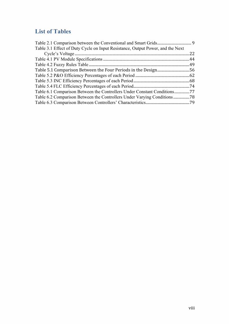
List of Tables Table 2.1 Comparison between the Conventional and Smart Grids....................................9Table 3.1 Effect of Duty Cycle on Input Resistance, Output Power, and the Next
Cycle’s Voltage.........................................................................................................................22Table 4.1 PV Module Specifications...........................................................................................44Table 4.2 Fuzzy Rules Table..........................................................................................................49Table5.1ComparisonBetweentheFourPeriodsintheDesign..................................56Table 5.2 P&O Efficiency Percentages of each Period.........................................................62Table 5.3 INC Efficiency Percentages of each Period...........................................................68Table 5.4FLC Efficiency Percentages of each Period...........................................................74Table 6.1 Comparison Between the Controllers Under Constant Conditions................77Table 6.2 Comparison Between the Controllers Under Varying Conditions.................78Table 6.3 Comparison Between Controllers’ Characteristics..............................................79
ix
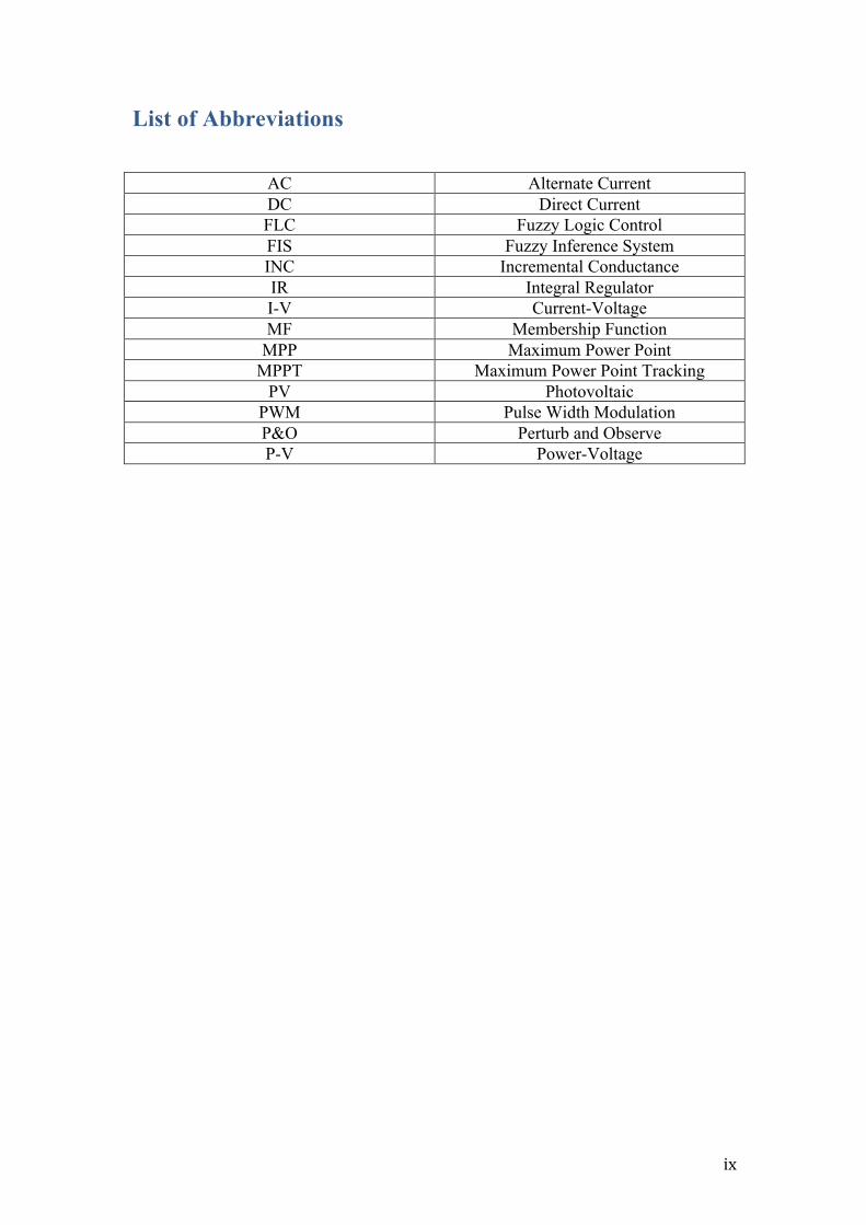
List of Abbreviations
AC Alternate Current DC Direct Current FLC Fuzzy Logic Control FIS Fuzzy Inference System INC Incremental Conductance IR Integral Regulator I-V Current-Voltage MF Membership Function
MPP Maximum Power Point MPPT Maximum Power Point Tracking
PV Photovoltaic PWM Pulse Width Modulation P&O Perturb and Observe P-V Power-Voltage

x
List of Publications
• M. Khallaf and A. Ismail, "Design and Simulation of Enhanced MPPT
Algorithms for Photovoltaic Systems", 10th IEEE GCC CONFERENCE,
Kuwait, April 2019.
• M. Khallaf and A. Ismail, "Design of Photovoltaic System using Fuzzy Logic
Controller", International Research Journal of Engineering and Technology
(IRJET), Volume 6 Issue 4, April 2019, S.NO: 296
1
Abstract Over the past years, the energy demand has been steadily growing and so methods of
how to cope with this staggering increase are being researched and utilized. One
method of injecting more energy to the grid is renewable energy, which has become
in recent years an integral part of any country’s power generation plan. Thus, it is a
necessity to enhance renewable energy resources and maximize their grid utilization,
so that these resources can step up and reduce the over dependency of global energy
production on depleting energy resources.
This thesis focuses on solar power and effective means to enhance its efficiency
through the use of different controllers. In this regard, substantial research efforts
have been done. However, due to the current market and technological development,
more options are made available that are able to boast the efficiency and utilization of
renewables in the power mix.
In this thesis, an enhanced maximum power point tracking (MPPT) controller has
been designed as part of a Photovoltaic (PV) system to generate maximum power to
satisfy load demand. The PV system is designed and simulated using MATLAB
(consisting of a solar panel array, MPPT controller, boost converter, and a resistive
load). The solar panel chosen for the array is Sun Power SPR- 440NE-WHT-D and
the array is designed to produce 150 kW of power. The MPPT controller is designed
using three different algorithms and the results are compared to identify each
controller’s fortes and drawbacks. The three designed controllers used are based on
Perturb and Observe (P&O) algorithm, Incremental Conductance (INC) with an
Integral Regulator (IR) and Fuzzy Logic Control (FLC). Each controller was tested
under two different scenarios; the first is when the panel array is subjected to constant

2
amount of solar irradiance along with a constant atmospheric temperature and the
second scenario has varying solar irradiance and atmospheric temperature. The
performance of these controllers is analyzed and compared in terms of the output
power efficiency, system dynamic response and finally the oscillations behavior.
After analyzing the results, it is shown that Fuzzy Logic Controller design performed
better compared to the other controllers as it had in most cases the highest mean
power efficiency and fastest response.

3
Chapter 1 Introduction
1.1 Motivation With the exponential growth in the human population and the expansion of cities
throughout the world, a predicament was born. How can electricity be supplied to
these new areas when the traditional grid is already failing at the current level of load?
The traditional energy system is becoming more and more unreliable by the day with
the increase in power outages, coal prices, greenhouse gas emissions and the amount
of electricity wasted during transmission through the grid for reasons ranging from
poor human oversight to natural disasters. Power blackouts are becoming a massive
burden and complication on the traditional grid. A power blackout is a failure to
deliver electricity to a certain area for a period of time and according to the US
Government, power outages and power quality issues cost American businesses more
than $100 billion on average each year [1]. It is also reported that the one-hour outage
in Chicago in 2000 resulted in $20 trillion in trades being delayed.
This has lead researchers to focus on developing new energy technologies that are
more reliable, robust, and have the ability to reduce the gas emissions and the loss of
electric power. Hence, the idea of Smart Grid was developed. This chapter describes
Smart Grids, examines their components, structure, and discusses their benefits and
challenges. This thesis focuses on the power generation components in smart grids
using solar energy.
4
1.2 Research Objectives Theobjectivesofthisresearcharesummarizedasfollows:
1. Designing an enhanced PV system that produces an output of 150 kW and
simulating it using a PV panel that is widely used in the industry (Sun Power
SPR- 440)
2. Designing three MPPT controllers: Perturb & Observe, Incremental
Conductance with Integral Regulator, and Fuzzy Logic.
3. Modeling and simulating the designed PV system using the three MPPT
controllers and compare their responses under constant and varying weather
conditions.
4. Studying the effect of increasing temperature and reducing irradiance on the
system output power.
1.3 Thesis Organization This Thesis is divided into six chapters, as follows:
• Chapter 1 describes the motivation behind this thesis and its objectives.
• Chapter 2 discusses the literature review behind Smart Grids and its main
components, especially the PV system, which is the main focus of this thesis.
• Chapter 3 discusses the three MPPT controllers used in this thesis, which are
P&O, INC+IR, and FLC.
• Chapter 4 shows the design of the PV system (PV Panel, MPPT, and DC-DC
Converters).
• Chapter 5 illustrates the results produced from each MPPT controller under
both constant and varying weather conditions.
• Chapter 6 summarizes the work done and the results obtained along with some
recommendations for further work.
5
Chapter 2 Problem Background
2.1 Introduction This chapter introduces two main topics, smart grids and renewable energy resources
(especially photovoltaic systems). It also highlights the structure, usage, and
challenges of implementing each of them individually.
2.2 Introduction to Smart Grids According to the U.S. Department of Energy, a Smart Grid is a digital technology that
allows two-way communication between consumers and the utility company. It also
makes use of the new control, automation, sensing, and communication technologies
integrated together to react to the unpredictable demand for electricity digitally and
without the aid of humans [2]. The National Electrical Manufacturers Association
(NEMA) also added a crucial point to the definition of Smart Grids, unlike the
traditional system, Smart Grids can take advantage of new technologies such as
distributed generation, renewable energy (solar, wind, etc.), smart metering, demand
side management systems, and distribution automation [3].
Smart Grids can also be used to combat all of the problems that emanate from the use
of a traditional grid due to the following features [1]:
• Smart Grid is intelligent due to its ability to anticipate and deal with overloads
autonomously and quicker than the workers would respond, which can lead to
decreasing or even averting power blackouts.
• Smart Grid is efficient as it can sense wastage in electricity and also keep up with
the ever-increasing demand in electricity without introducing extra power lines.

6
• Smart Grid can accommodate renewable energy because it can smoothly integrate
any type of energy resource such as renewable energy sources to handle part of
the load and thus limiting the usage of coal and natural gas, which will reduce our
carbon footprint.
• Smart Grid is engaging as it actively links the consumer with the utility company,
which allows the consumer to control their power consumption in terms of price
and source of power (coal, solar, etc.)
• Smart Grid is resilient as it is more distributed than centralized and with the
inclusion of the safety procedures it becomes a lot more withstanding.
• Finally, Smart Grid is more environmentally friendly due to the advanced
technologies incorporated within renewable energy sources that can now be easily
integrated with the grid thus reducing the CO2 emissions and global warming.
The basic requirements of a Smart Grid are: (i) integrated communication platform
that can interconnect all the different components in the system and allow for the
exchange of data; (ii) an abundance of sensors and measuring devices to record every
action precisely and in real time for the use of either the utility company or the
consumer; (iii) advanced control and automation techniques to correctly predict the
ever-changing demand for electricity and to be able to cope and react to any
unforeseen event swiftly; (iv) latest technology in energy storage and electronics to
amplify the overall performance and efficiency of the system; and (v) a high-level
software or artificial intelligence (AI) based system to gather information, decide
which course of action is needed to be taken and relay it to the system.
7
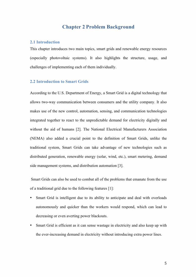
Figure 2.1 Smart Grid Components [4]
The components of a Smart Grid, shown in Figure 2.1, can be summarized as follows
[5]:
(i) Sensors: these components need to be placed across the network on each
transmission line and transformer. There are many types of sensors such as
voltage, current, temperature, and fault indication to keep the workers alert
on what is going on during transmission at all times. This information will
be sent back to the monitoring station over the wireless communication
system.
(ii) Communication System: this system would need to be a WAN (Wide Area
Network) to be able to cover all the distance from the generation station to
the end of the line whether it is a house, commercial building, government
entity or an industrial site.
(iii) Distribution Management system: this component includes Distribution
Automation, Distribution Generation, Fault Management and other
supervisory purposes. This part of the grid is a very critical part as it is the
8
starting point from which the consumer gets electricity; therefore, there are
a lot of variables that need monitoring and optimizing. This part of the grid
will be sending out data regarding power generation, power quality, power
flow, the usual measurements of voltage and current, and finally the status
of the advanced electronics used in the system all in real time, which
necessitates handling this system with additional caution and upkeep.
(iv) Control Technology is needed to adapt to a calculated switching
operations of the network as well as a deliberate isolation or cutting off
power during the times of low demand for electricity. At first, the task
handled by the control system may seem simple, but this system needs to
be of a high dependability and promptness. During sudden emergencies,
ones that take precedence over regular and daily functions; the control
technology used should be able to adjust itself to shoulder its daily
functions along with the emergency response immediately to prevent a
catastrophe from occurring.
(v) Advanced Metering Infrastructure (AMI): which are smart meters situated
at the consumers’ place. This advanced technology also uses the wireless
communication function to provide the utility company with real-time data
regarding power consumption and power irregularities so that it can
predict and act accordingly ahead of time. It also benefits the user as it
provides data about the change in price depending on time and also
regarding future power outages.
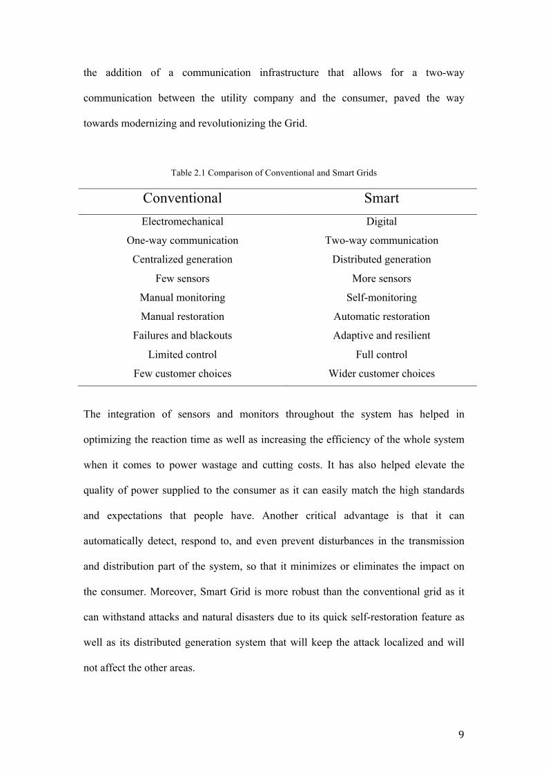
Table 2.1 shows main differences between the conventional Grids and Smart Grids.
The transformation from an electromechanical system into a digital system along with
9
the addition of a communication infrastructure that allows for a two-way
communication between the utility company and the consumer, paved the way
towards modernizing and revolutionizing the Grid.
Table 2.1 Comparison of Conventional and Smart Grids
Conventional Smart Electromechanical Digital
One-way communication Two-way communication
Centralized generation Distributed generation
Few sensors More sensors
Manual monitoring Self-monitoring
Manual restoration Automatic restoration
Failures and blackouts Adaptive and resilient
Limited control Full control
Few customer choices Wider customer choices
The integration of sensors and monitors throughout the system has helped in
optimizing the reaction time as well as increasing the efficiency of the whole system
when it comes to power wastage and cutting costs. It has also helped elevate the
quality of power supplied to the consumer as it can easily match the high standards
and expectations that people have. Another critical advantage is that it can
automatically detect, respond to, and even prevent disturbances in the transmission
and distribution part of the system, so that it minimizes or eliminates the impact on
the consumer. Moreover, Smart Grid is more robust than the conventional grid as it
can withstand attacks and natural disasters due to its quick self-restoration feature as
well as its distributed generation system that will keep the attack localized and will
not affect the other areas.

10
Smart Grid will also help in integrating the technologies of the 21st Century such as
electric and hybrid cars due to the integration of renewable energy as well as
advanced storage technologies that will allow us access to plug-in from virtually
everywhere [6]. Finally, a subtle benefit of implementing Smart Grids is that it
actually opens up a new space in a market that is becoming more and more saturated
by the day. Should Smart Grids be implemented heavily in the future, this will cause
a huge demand worldwide: a demand for electronics, communication, control
technologies, and also human capital. Smart Grids are considered an immense
investment and commitment that will not only gear us towards a better future but will
also change the lives of all people right now from the lowest ranking worker to the
biggest investing company. Everyone will have a chance to improve his or her quality
of life.
2.2.1 Challenges of a Smart Grid Even though Smart Grids have the capability of transforming the electric energy
market, designing and implementing it are two different things. There are some
challenges that need to be tackled after committing to the decision of improving their
grid structure. Some palpable challenges are the high initial cost and the amount of
time needed to transform the grid. Another challenge is the advanced technology
factor. Smart Grids depend hugely on advanced technologies in every field:
electronics, communication, control and automation, AMI, storage devices, and
software-wise as well. These kinds of technologies are hard to come by as they are
either very costly, or hard to acquire or purchase.
Furthermore, another major challenge is cyber security. With the grid transformed
into a digital one and everything being controlled or monitored wirelessly, the threat
of having someone hack into it is now a huge possibility. To overcome such a
11
problem, a high-level security protocol with multiple firewalls must be used like the
one used by the US Federal Aviation Administration to protect the landing and taking
off of planes.
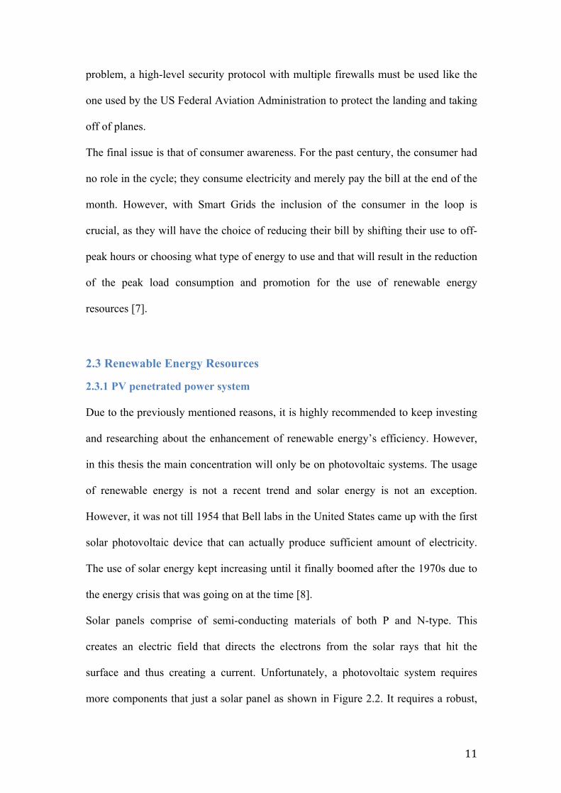
The final issue is that of consumer awareness. For the past century, the consumer had
no role in the cycle; they consume electricity and merely pay the bill at the end of the
month. However, with Smart Grids the inclusion of the consumer in the loop is
crucial, as they will have the choice of reducing their bill by shifting their use to off-
peak hours or choosing what type of energy to use and that will result in the reduction
of the peak load consumption and promotion for the use of renewable energy
resources [7].
2.3 Renewable Energy Resources
2.3.1 PV penetrated power system Due to the previously mentioned reasons, it is highly recommended to keep investing
and researching about the enhancement of renewable energy’s efficiency. However,
in this thesis the main concentration will only be on photovoltaic systems. The usage
of renewable energy is not a recent trend and solar energy is not an exception.
However, it was not till 1954 that Bell labs in the United States came up with the first
solar photovoltaic device that can actually produce sufficient amount of electricity.
The use of solar energy kept increasing until it finally boomed after the 1970s due to
the energy crisis that was going on at the time [8].
Solar panels comprise of semi-conducting materials of both P and N-type. This
creates an electric field that directs the electrons from the solar rays that hit the
surface and thus creating a current. Unfortunately, a photovoltaic system requires
more components that just a solar panel as shown in Figure 2.2. It requires a robust,
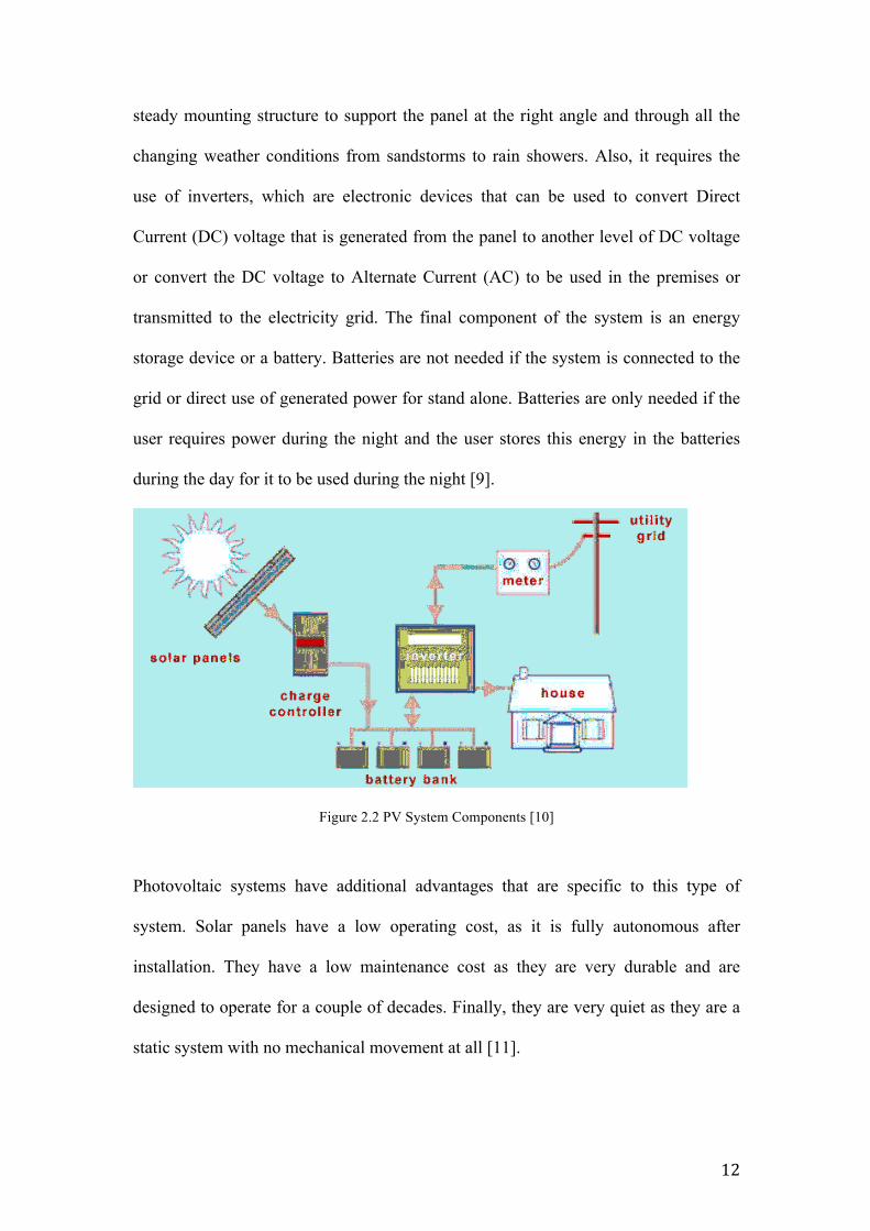
12
steady mounting structure to support the panel at the right angle and through all the
changing weather conditions from sandstorms to rain showers. Also, it requires the
use of inverters, which are electronic devices that can be used to convert Direct
Current (DC) voltage that is generated from the panel to another level of DC voltage
or convert the DC voltage to Alternate Current (AC) to be used in the premises or
transmitted to the electricity grid. The final component of the system is an energy
storage device or a battery. Batteries are not needed if the system is connected to the
grid or direct use of generated power for stand alone. Batteries are only needed if the
user requires power during the night and the user stores this energy in the batteries
during the day for it to be used during the night [9].
Figure 2.2 PV System Components [10]
Photovoltaic systems have additional advantages that are specific to this type of
system. Solar panels have a low operating cost, as it is fully autonomous after
installation. They have a low maintenance cost as they are very durable and are
designed to operate for a couple of decades. Finally, they are very quiet as they are a
static system with no mechanical movement at all [11].
13
2.3.2 PV Penetrated Power System Challenging Issues Even though Photovoltaic system is the most widely used type of renewable energy, it
still has quite a few downsides that are still under research and enhancement.
2.3.2.1PVIntermittentNatureOne of the biggest issues with using photovoltaic technology is that it is dependent on
weather conditions or to be more specific, on the amount and direction of solar rays
reaching the surface of the panel. This makes it highly unpredictable and in some
cases unreliable. Another major problem is the percentage efficiency or the
conversion rate of the photovoltaic module. Solar panels have one of the least
efficiency percentages compared to other energy generating technologies, where the
average solar panel converts only 16% into electricity with a range of 12% to 22%.
Hence, a large number of panels needed to be installed to compensate for this
efficiency. However other electronic devices need to be used such as inverters and
energy storage batteries.
The usage of high numbers of solar panels leads to the next problem, which is the area
used to install the solar panels and its additional components. Installing solar panels
on rooftops is acceptable as it makes use of unutilized areas, however to generate an
adequate amount of solar power a vast area of land is needed.
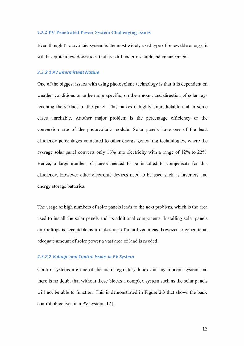
2.3.2.2VoltageandControlIssuesinPVSystem
Control systems are one of the main regulatory blocks in any modern system and
there is no doubt that without these blocks a complex system such as the solar panels
will not be able to function. This is demonstrated in Figure 2.3 that shows the basic
control objectives in a PV system [12].
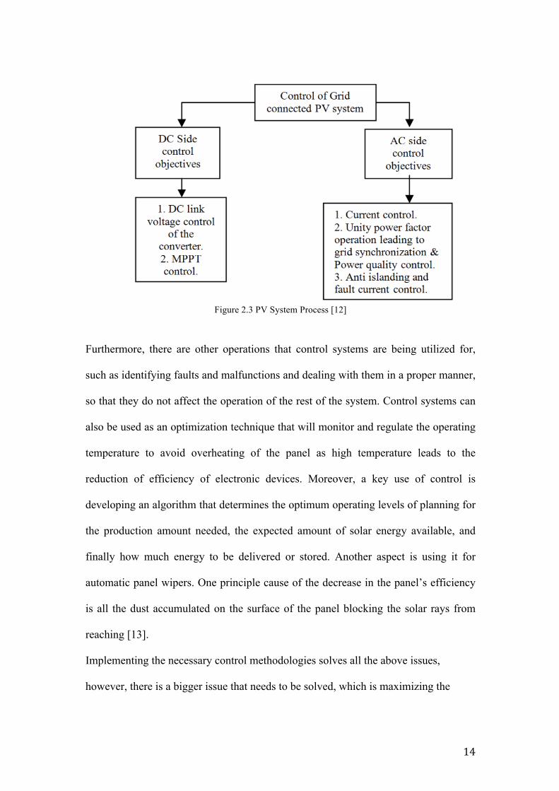
14
Figure 2.3 PV System Process [12]
Furthermore, there are other operations that control systems are being utilized for,
such as identifying faults and malfunctions and dealing with them in a proper manner,
so that they do not affect the operation of the rest of the system. Control systems can
also be used as an optimization technique that will monitor and regulate the operating
temperature to avoid overheating of the panel as high temperature leads to the
reduction of efficiency of electronic devices. Moreover, a key use of control is
developing an algorithm that determines the optimum operating levels of planning for
the production amount needed, the expected amount of solar energy available, and
finally how much energy to be delivered or stored. Another aspect is using it for
automatic panel wipers. One principle cause of the decrease in the panel’s efficiency
is all the dust accumulated on the surface of the panel blocking the solar rays from
reaching [13].
Implementing the necessary control methodologies solves all the above issues,
however, there is a bigger issue that needs to be solved, which is maximizing the

15
output power problem. Using an MPPT controller, which is discussed in the next
section, can solve this issue.
2.3.3 Maximum Power Point Tracking (MPPT) The MPPT is used to study the naturally low efficiency of the solar cells and seeks to
keep the output power as high as possible at all times, especially during varying
weather conditions. There are many different MPPT techniques that are used under
different circumstances and yield different outputs as well. However, this thesis will
focus on three specific techniques: (i) Perturb and Observe; (ii) Incremental
Conductance; and (iii) Fuzzy Logic Control. All MPPT techniques are responsible for
finding the best and highest combination of the panel’s voltage and current to get the
optimum level of power.
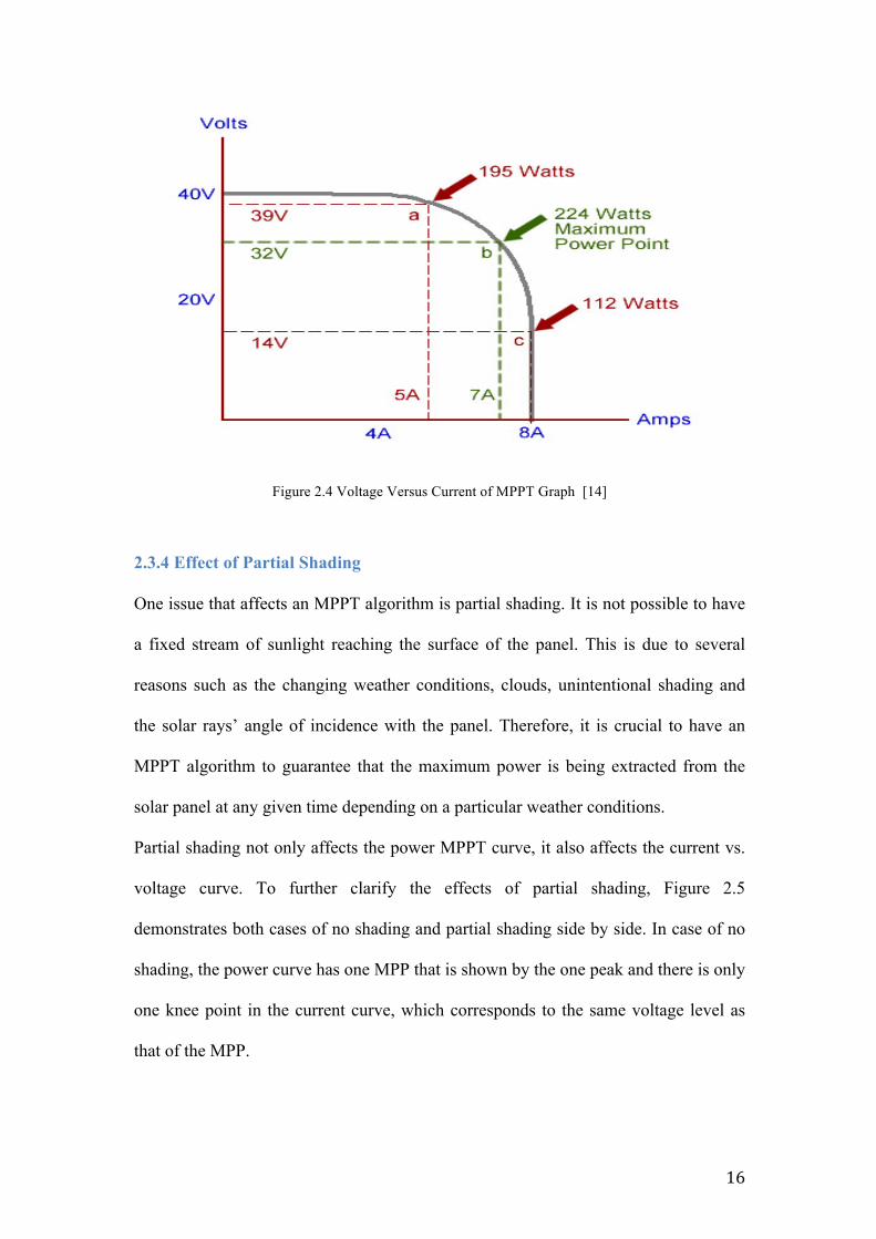
The voltage versus current of the MPPT graph is presented in Figure 2.4, which
shows multiple points including the maximum power point. There are three points
that are shown on the curve: point A, B, and C. Point A depicts the power output
when using a voltage level of 39 Volts and a current level of 5 Amperes, which
produces 195 W of power. Point C has a voltage level of 14 Volts and a current level
of 7 Amperes, which produces a power output of 112 W. Points A and C are at the top
and bottom of the curve respectively, however, neither of them is the MPP. The MPP
is located at the knee point of the curve in between points A and C, which is point B.
Point B has a voltage level of 32 Volts and a current level of 7 Amperes, which when
multiplied together give a power output of 224 W. Since this is the point where the
power output is at its highest, it is called the MPP. Chapter 3 is dedicated to
explaining the MPPT and the three control techniques that are used in the design of
this Thesis.
16
Figure 2.4 Voltage Versus Current of MPPT Graph [14]
2.3.4 Effect of Partial Shading One issue that affects an MPPT algorithm is partial shading. It is not possible to have
a fixed stream of sunlight reaching the surface of the panel. This is due to several
reasons such as the changing weather conditions, clouds, unintentional shading and
the solar rays’ angle of incidence with the panel. Therefore, it is crucial to have an
MPPT algorithm to guarantee that the maximum power is being extracted from the
solar panel at any given time depending on a particular weather conditions.
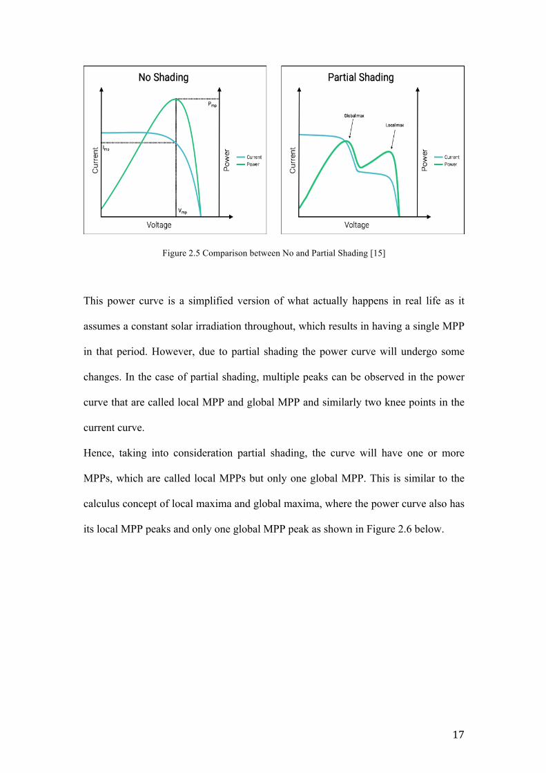
Partial shading not only affects the power MPPT curve, it also affects the current vs.
voltage curve. To further clarify the effects of partial shading, Figure 2.5
demonstrates both cases of no shading and partial shading side by side. In case of no
shading, the power curve has one MPP that is shown by the one peak and there is only
one knee point in the current curve, which corresponds to the same voltage level as
that of the MPP.
17
Figure 2.5 Comparison between No and Partial Shading [15]
This power curve is a simplified version of what actually happens in real life as it
assumes a constant solar irradiation throughout, which results in having a single MPP
in that period. However, due to partial shading the power curve will undergo some
changes. In the case of partial shading, multiple peaks can be observed in the power
curve that are called local MPP and global MPP and similarly two knee points in the
current curve.
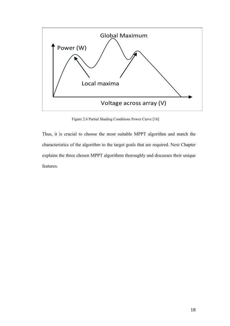
Hence, taking into consideration partial shading, the curve will have one or more
MPPs, which are called local MPPs but only one global MPP. This is similar to the
calculus concept of local maxima and global maxima, where the power curve also has
its local MPP peaks and only one global MPP peak as shown in Figure 2.6 below.
18
Figure 2.6 Partial Shading Conditions Power Curve [16]
Thus, it is crucial to choose the most suitable MPPT algorithm and match the
characteristics of the algorithm to the target goals that are required. Next Chapter
explains the three chosen MPPT algorithms thoroughly and discusses their unique
features.
19
Chapter 3 MPPT Controllers This chapter sheds light on the most common methods and algorithms that are used
for MPPT in PV applications. The three types of proposed controllers used are:
Perturb & Observe, Incremental Conductance with Integral Regulator, and Fuzzy
Logic. As previously mentioned, MPPT techniques are used to ensure the
maximization of the system’s output power at all times.
3.1 Perturb & Observe Algorithm
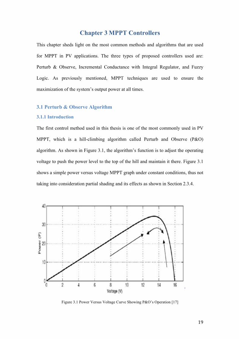
3.1.1 Introduction The first control method used in this thesis is one of the most commonly used in PV
MPPT, which is a hill-climbing algorithm called Perturb and Observe (P&O)
algorithm. As shown in Figure 3.1, the algorithm’s function is to adjust the operating
voltage to push the power level to the top of the hill and maintain it there. Figure 3.1
shows a simple power versus voltage MPPT graph under constant conditions, thus not
taking into consideration partial shading and its effects as shown in Section 2.3.4.
Figure 3.1 Power Versus Voltage Curve Showing P&O’s Operation [17]
20
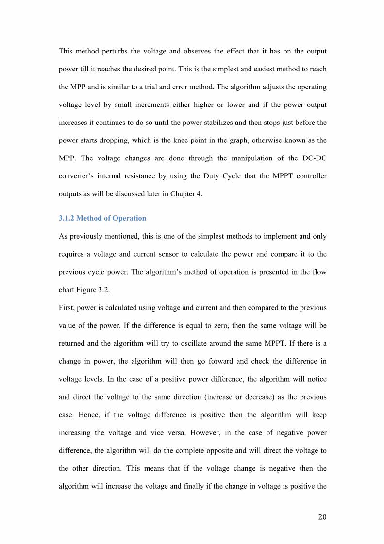
This method perturbs the voltage and observes the effect that it has on the output
power till it reaches the desired point. This is the simplest and easiest method to reach
the MPP and is similar to a trial and error method. The algorithm adjusts the operating
voltage level by small increments either higher or lower and if the power output
increases it continues to do so until the power stabilizes and then stops just before the
power starts dropping, which is the knee point in the graph, otherwise known as the
MPP. The voltage changes are done through the manipulation of the DC-DC
converter’s internal resistance by using the Duty Cycle that the MPPT controller
outputs as will be discussed later in Chapter 4.
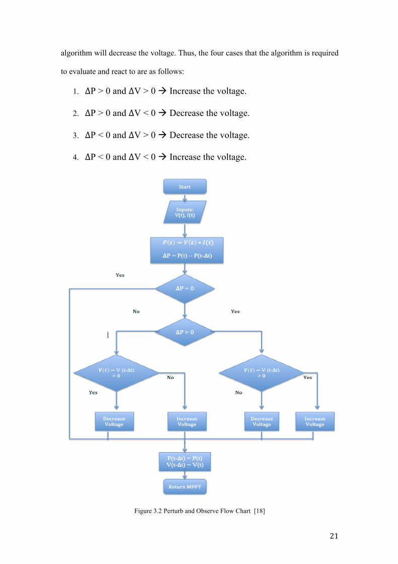
3.1.2 Method of Operation As previously mentioned, this is one of the simplest methods to implement and only
requires a voltage and current sensor to calculate the power and compare it to the
previous cycle power. The algorithm’s method of operation is presented in the flow
chart Figure 3.2.
First, power is calculated using voltage and current and then compared to the previous
value of the power. If the difference is equal to zero, then the same voltage will be
returned and the algorithm will try to oscillate around the same MPPT. If there is a
change in power, the algorithm will then go forward and check the difference in
voltage levels. In the case of a positive power difference, the algorithm will notice
and direct the voltage to the same direction (increase or decrease) as the previous
case. Hence, if the voltage difference is positive then the algorithm will keep
increasing the voltage and vice versa. However, in the case of negative power
difference, the algorithm will do the complete opposite and will direct the voltage to
the other direction. This means that if the voltage change is negative then the
algorithm will increase the voltage and finally if the change in voltage is positive the
21
algorithm will decrease the voltage. Thus, the four cases that the algorithm is required
to evaluate and react to are as follows:
1. ∆P > 0 and ∆V > 0 à Increase the voltage.
2. ∆P > 0 and ∆V < 0 à Decrease the voltage.
3. ∆P < 0 and ∆V > 0 à Decrease the voltage.
4. ∆P < 0 and ∆V < 0 à Increase the voltage.
Figure 3.2 Perturb and Observe Flow Chart [18]
22
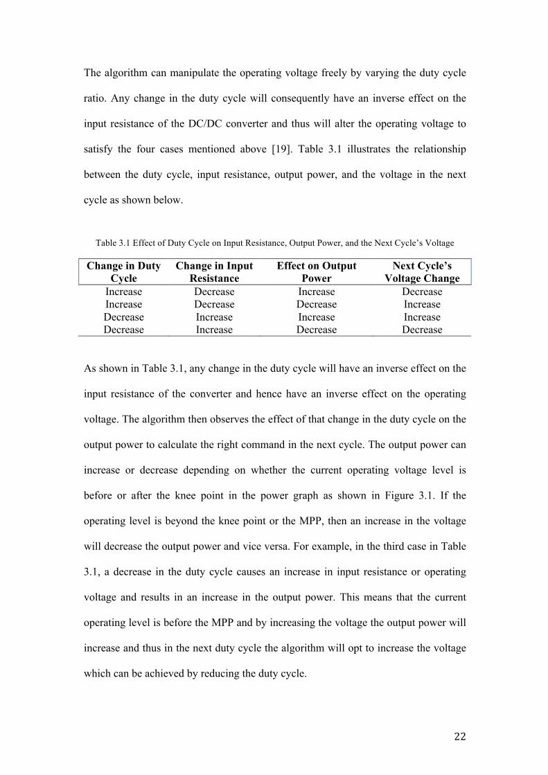
The algorithm can manipulate the operating voltage freely by varying the duty cycle
ratio. Any change in the duty cycle will consequently have an inverse effect on the
input resistance of the DC/DC converter and thus will alter the operating voltage to
satisfy the four cases mentioned above [19]. Table 3.1 illustrates the relationship
between the duty cycle, input resistance, output power, and the voltage in the next
cycle as shown below.
Table 3.1 Effect of Duty Cycle on Input Resistance, Output Power, and the Next Cycle’s Voltage
Change in Duty Cycle
Change in Input Resistance
Effect on Output Power
Next Cycle’s Voltage Change
Increase Decrease Increase Decrease Increase Decrease Decrease Increase Decrease Increase Increase Increase Decrease Increase Decrease Decrease
As shown in Table 3.1, any change in the duty cycle will have an inverse effect on the
input resistance of the converter and hence have an inverse effect on the operating
voltage. The algorithm then observes the effect of that change in the duty cycle on the
output power to calculate the right command in the next cycle. The output power can
increase or decrease depending on whether the current operating voltage level is
before or after the knee point in the power graph as shown in Figure 3.1. If the
operating level is beyond the knee point or the MPP, then an increase in the voltage
will decrease the output power and vice versa. For example, in the third case in Table
3.1, a decrease in the duty cycle causes an increase in input resistance or operating
voltage and results in an increase in the output power. This means that the current
operating level is before the MPP and by increasing the voltage the output power will
increase and thus in the next duty cycle the algorithm will opt to increase the voltage
which can be achieved by reducing the duty cycle.
23
3.1.3 Advantages and disadvantages of P&O method Perturb and Observe method is a widely known hill-climbing method for several
reasons. Firstly, it is the most simplistic algorithm for MPPT and only requires one
voltage sensor. For that reason, it is a fast, inexpensive, and easy to implement option.
Secondly, unlike the other MPPT algorithms that will be discussed further on, P&O
method has a short computing time and a low computing complexity as it does not
require any mathematical calculations. Only a comparison of the current and previous
voltage and power values is required. This enables P&O to decide which side the
current level is on with respect to the knee point and to move the voltage in the
correct direction swiftly. However, this simplistic approach has its failures especially
when dealing with a complex system such as a PV array. The first downside to this
algorithm is that, given its method of operation, the voltage level never stays in the
same level even when the MPP is reached similar to the power level. The algorithm
cannot help but continue to perturb. Once it reaches around the MPP it decreases the
perturb magnitude but that still causes significant power loss compared to the other
algorithms. Another disadvantage of using P&O is the way it responds to the
continuously changing weather conditions [20]. As the weather changes and the
irradiance hitting the panel’s surface increases, the MPP automatically shifts to the
right as shown in Figure 3.3.
24
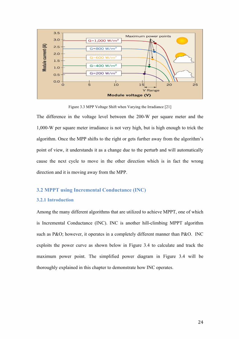
Figure 3.3 MPP Voltage Shift when Varying the Irradiance [21]
The difference in the voltage level between the 200-W per square meter and the
1,000-W per square meter irradiance is not very high, but is high enough to trick the
algorithm. Once the MPP shifts to the right or gets further away from the algorithm’s
point of view, it understands it as a change due to the perturb and will automatically
cause the next cycle to move in the other direction which is in fact the wrong
direction and it is moving away from the MPP.
3.2 MPPT using Incremental Conductance (INC)
3.2.1 Introduction Among the many different algorithms that are utilized to achieve MPPT, one of which
is Incremental Conductance (INC). INC is another hill-climbing MPPT algorithm
such as P&O; however, it operates in a completely different manner than P&O. INC
exploits the power curve as shown below in Figure 3.4 to calculate and track the
maximum power point. The simplified power diagram in Figure 3.4 will be
thoroughly explained in this chapter to demonstrate how INC operates.
25
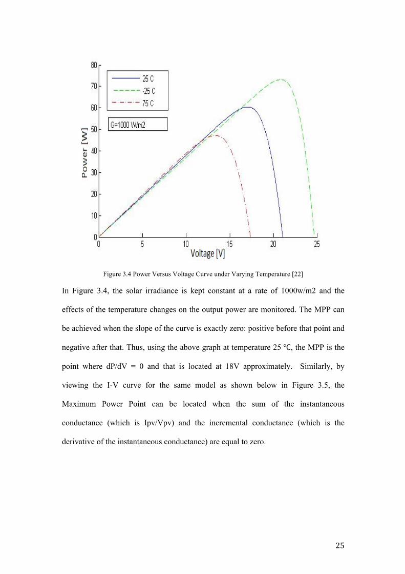
Figure 3.4 Power Versus Voltage Curve under Varying Temperature [22]
In Figure 3.4, the solar irradiance is kept constant at a rate of 1000w/m2 and the
effects of the temperature changes on the output power are monitored. The MPP can
be achieved when the slope of the curve is exactly zero: positive before that point and
negative after that. Thus, using the above graph at temperature 25 ℃, the MPP is the
point where dP/dV = 0 and that is located at 18V approximately. Similarly, by
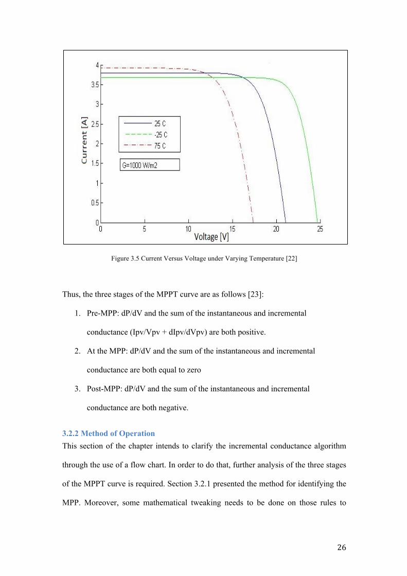
viewing the I-V curve for the same model as shown below in Figure 3.5, the
Maximum Power Point can be located when the sum of the instantaneous
conductance (which is Ipv/Vpv) and the incremental conductance (which is the
derivative of the instantaneous conductance) are equal to zero.
26
Figure 3.5 Current Versus Voltage under Varying Temperature [22]
Thus, the three stages of the MPPT curve are as follows [23]:
1. Pre-MPP: dP/dV and the sum of the instantaneous and incremental
conductance (Ipv/Vpv + dIpv/dVpv) are both positive.
2. At the MPP: dP/dV and the sum of the instantaneous and incremental
conductance are both equal to zero
3. Post-MPP: dP/dV and the sum of the instantaneous and incremental
conductance are both negative.
3.2.2 Method of Operation
This section of the chapter intends to clarify the incremental conductance algorithm
through the use of a flow chart. In order to do that, further analysis of the three stages
of the MPPT curve is required. Section 3.2.1 presented the method for identifying the
MPP. Moreover, some mathematical tweaking needs to be done on those rules to
27
understand what gets fed into the MPPT controller. As previously mentioned, there
are three stages in the curve:
1. Pre- MPP: dP/dV is positive.
2. At the MPP: dP/dV is equal to zero
3. Post MPP: dP/dV is negative.
Since P = IV, thus dP/dV = dI*V/dV. (3.1)
Equation 3.1 leads to:
(V* dI/dV) + I (3.2)
Further manipulation will result in:
dI/dV = -I/V (3.3)
Thus, applying equation 3.3 on the three stages results in:
1. Pre- MPP: dI/dV > -I/V
2. At the MPP: dI/dV = -I/V
3. Post MPP: dI/dV < -I/V
The above calculations are meant to provide an understanding of the algorithm’s
inputs at the sensor level of the circuit. It demonstrates that in order for the algorithm
to locate the MPP, it compares the values of the change in I/V with -I/V until both are
equal and that is when it reaches the MPP.
After clarifying the inputs of the algorithm and how they are utilized, the next step is
mapping out the flow chart of the algorithm’s cycle. The flowchart in Figure 3.6
shows the sequence of steps for the algorithm.
The starting point of the flowchart is to input the values of both the current and the
voltage outputs of the PV array. The step of updating the voltage and current of the
PV array is done intermittently depending on the chosen duty cycle. As soon as the
controller receives these inputs, it evaluates and compares them with the previous
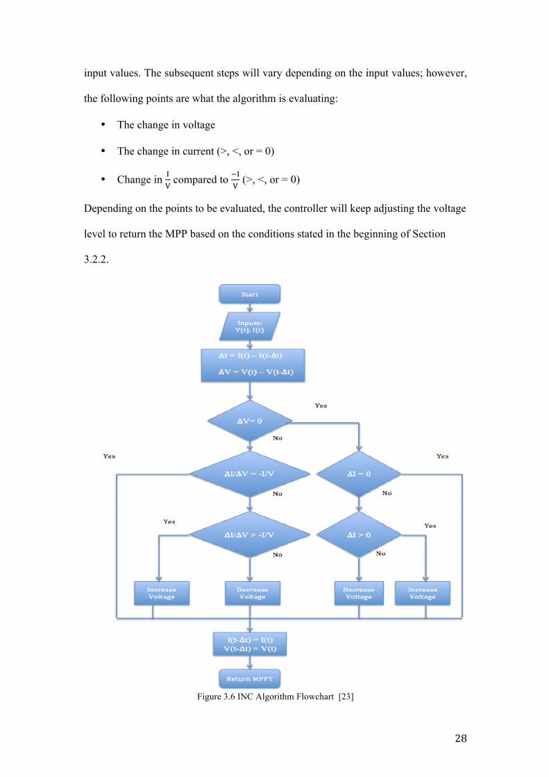
28
input values. The subsequent steps will vary depending on the input values; however,
the following points are what the algorithm is evaluating:
• The change in voltage
• The change in current (>, <, or = 0)
• Change in !! compared to !!
! (>, <, or = 0)
Depending on the points to be evaluated, the controller will keep adjusting the voltage
level to return the MPP based on the conditions stated in the beginning of Section
3.2.2.
Figure 3.6 INC Algorithm Flowchart [23]
29
3.2.3 Advantages and Disadvantages of INC Incremental conductance is one of the commonly used hill-climbing algorithms in
MPPT controller and there are several reasons behind that. First and foremost is the
method of tracking the MPP. As discussed in the previous sections, INC has
successfully divided the PV power output graph into three sections Pre-MPP, MPP
and Post-MPP. Each of these sections has a unique value for dP/dV: positive, zero,
and negative. Thus by exploiting these facts, INC has a clear advantage over the P&O
algorithm, which is the computational time and accuracy of the MPP. During
changing weather conditions, the P&O method will keep on oscillating to get close
and locate the MPP. However, using INC, no oscillations are required and the
algorithm knows exactly which stage of the previously mentioned three it is in and
will increment or decrement the voltage immediately until it reaches the zero slope,
which is the MPP and thus, the computational time is reduced. Another advantage is
the higher accuracy when it comes to tracking MPP. Unlike P&O that oscillates
around the MPP, INC is able to pinpoint the location of the MPP, which means it has
a higher efficiency. The two downsides of using INC are the complexity and the
possible inaccuracy. Even though INC is much less complex than Fuzzy logic, it is
still more complex to implement than P&O. Furthermore, when it comes to MPPT it
is not the best algorithm to be used but it is superior to that of the P&O. When it
comes to choosing which algorithm to be used for MPPT, there is always a tradeoff,
speed and efficiency on one hand and complexity and price on the other one.
3.2.4 INC Coupled with Integral Regulator (IR) The target of the MPPT is to track and locate the global MPP since it has the highest
efficiency. However most tracking techniques might mistake the local MPP with a
30
global MPP and thus it will take longer to track and it might need more advanced
algorithms for better tracking of the global MPP.
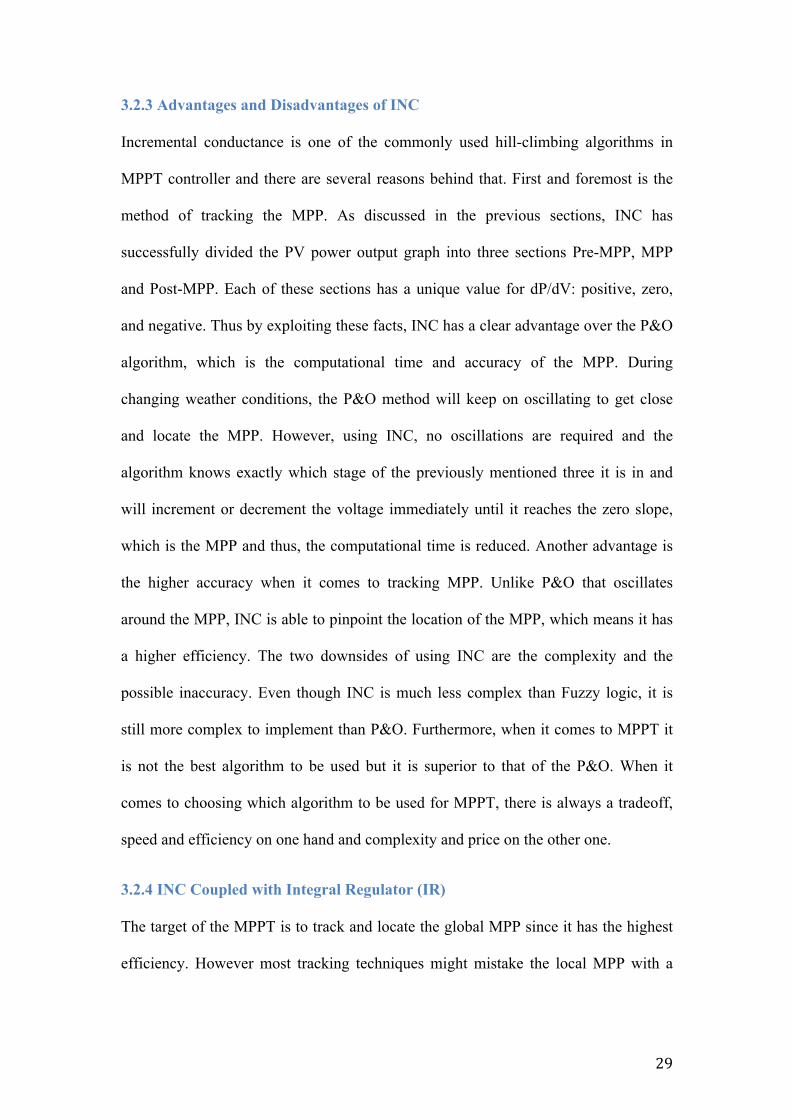
To combat both the efficiency concern and to try and reduce the time needed to locate
the global maximum, an integral regulator was used along with the incremental
conductance algorithm as shown in Figure 3.7. This figure illustrates that the addition
of the integral regulator adds an extra step between the MPPT algorithm and the
PWM generator. The integral regulator is used to increase the output efficiency by
performing duty cycle correction. This allows for more control, grip, and adaptation
with the ever-changing weather conditions that affect the MPP and hence increase the
system efficiency.
Figure 3.7 MPPT with Integral Regulator
This adaptive method increases the system efficiency using three key factors. Firstly,
the IR improves the method of operation of the incremental conductance by reducing
the error between the instantaneous conductance and the incremental conductance (as
discussed in Section 3.2.1). Secondly, as another hill-climbing method like the P&O
31
algorithm, the INC suffers from constant oscillations or ripples in the output. Adding
the integral regulator can reduce these ripples, which will also result in a better digital
resolution of the output. Lastly, the integral regulator improves the accuracy of both
the system’s large step sizes for when the operating level is far from the MPP and also
the small step sizes when the MPP is reached to extract the highest possible level of
power [24].
3.3 MPPT Using Fuzzy Logic Controller
3.3.1 Introduction to Fuzzy Logic Fuzzy logic is considered a type of many-valued logic (MVL) or otherwise called
non-classical logic. They are a form of logic that do not constrain the output truth-
values to only two but accept the range of values in between as well [25]. This means
that it not restricted to binary values of “0” and “1” or “True” and “False”, but
operates as well in the grey area in between allowing for a more accurate indication of
the variable. Another unique attribute that fuzzy logic has is the use of linguistic
interpretation instead of numerical, which makes it closer to the human thought
process. When Lukasiewicz and Tarski introduced infinite-valued logic in 1920 and
when Lotfi Zadeh perfected it and introduced fuzzy Logic in 1965, they all knew that
a new framework that is not only black and white was needed [26].
3.3.2 Fuzzy Sets and Membership Functions
Fuzzy logic is a unique method that transforms mathematical equations into a set of
linguistic commands which is done using two crucial aspects: fuzzy sets and
membership functions. Fuzzy sets are a group of sets where the numerical data gets
allocated to, and by doing so it transforms numerical values into linguistic ones.
Fuzzy sets are similar to the Mathematical concept of having a universe of discourse,
32
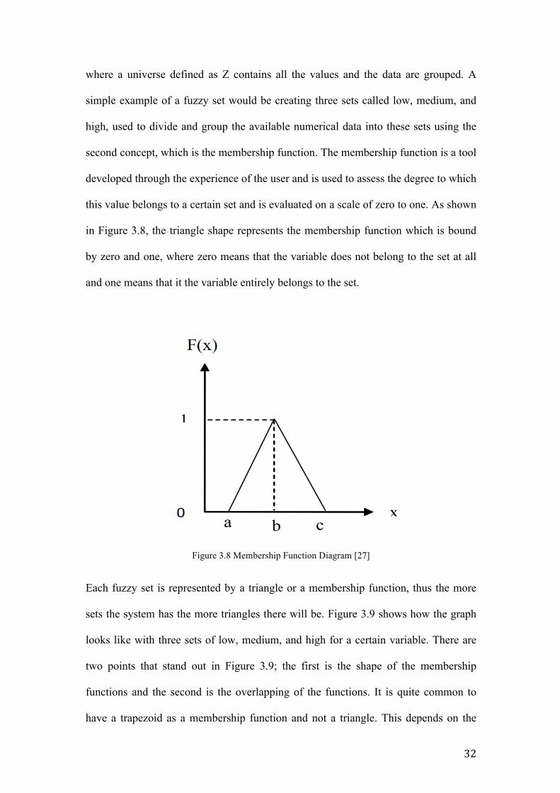
where a universe defined as Z contains all the values and the data are grouped. A
simple example of a fuzzy set would be creating three sets called low, medium, and
high, used to divide and group the available numerical data into these sets using the
second concept, which is the membership function. The membership function is a tool
developed through the experience of the user and is used to assess the degree to which
this value belongs to a certain set and is evaluated on a scale of zero to one. As shown
in Figure 3.8, the triangle shape represents the membership function which is bound
by zero and one, where zero means that the variable does not belong to the set at all
and one means that it the variable entirely belongs to the set.
Figure 3.8 Membership Function Diagram [27]
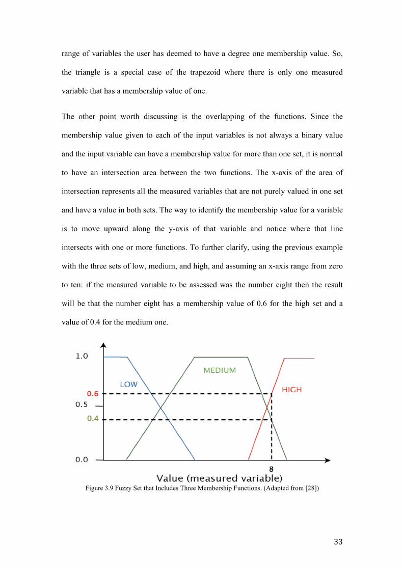
Each fuzzy set is represented by a triangle or a membership function, thus the more
sets the system has the more triangles there will be. Figure 3.9 shows how the graph
looks like with three sets of low, medium, and high for a certain variable. There are
two points that stand out in Figure 3.9; the first is the shape of the membership
functions and the second is the overlapping of the functions. It is quite common to
have a trapezoid as a membership function and not a triangle. This depends on the
33
range of variables the user has deemed to have a degree one membership value. So,
the triangle is a special case of the trapezoid where there is only one measured
variable that has a membership value of one.
The other point worth discussing is the overlapping of the functions. Since the
membership value given to each of the input variables is not always a binary value
and the input variable can have a membership value for more than one set, it is normal
to have an intersection area between the two functions. The x-axis of the area of
intersection represents all the measured variables that are not purely valued in one set
and have a value in both sets. The way to identify the membership value for a variable
is to move upward along the y-axis of that variable and notice where that line
intersects with one or more functions. To further clarify, using the previous example
with the three sets of low, medium, and high, and assuming an x-axis range from zero
to ten: if the measured variable to be assessed was the number eight then the result
will be that the number eight has a membership value of 0.6 for the high set and a
value of 0.4 for the medium one.
Figure 3.9 Fuzzy Set that Includes Three Membership Functions. (Adapted from [28])
34
3.3.3 Fuzzy Rules and Reasoning
A fuzzy set can be adapted and tailored towards any application and that is due to the
fuzzy rules that are embedded in each of the sets. A fuzzy rule is a statement
developed by the user of the logic based on the knowledge of the industry experts to
determine the output based on the input variables. These rules are formulated as
conditional statements that utilize the “if” and “then” arguments along with some
logic gates as well such as “and”, “not” and “or” [29]. The rules were built in such a
way to mimic the day-to-day human reasoning that is being done naturally such as “IF
room temperature is low THEN switch the air-conditioning to low.” In this
conditioning statement, the “if” and “then” argument was used to figure out the output
and input. In this case, the output is the air-conditioning fan level and the input is the
room temperature. The final elements of the rule are the fuzzy sets that represent both
the input and the output values, which in this case are both called low. A general
fuzzy rule should look like equation 3.4:
IF X is FS THEN Y is FS (3.4)
Where:
X is the input measured variable.
FS is the Fuzzy Set assigned to each variable.
Y is the output measured variable.
Equation 3.4 is the most general and simplified version of the fuzzy rule but as the
application gets more and more complicated slight changes can be noticed on the rule
such as the number of inputs, the number of outputs, and finally the number of
conditions in the rule.
Now that the fuzzy rules have been explained, the next part is to understand how the
user programs the set of fuzzy rules so that fuzzy logic can calculate the output from
35
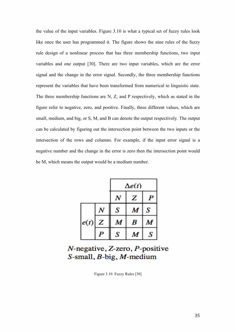
the value of the input variables. Figure 3.10 is what a typical set of fuzzy rules look
like once the user has programmed it. The figure shows the nine rules of the fuzzy
rule design of a nonlinear process that has three membership functions, two input
variables and one output [30]. There are two input variables, which are the error
signal and the change in the error signal. Secondly, the three membership functions
represent the variables that have been transformed from numerical to linguistic state.
The three membership functions are N, Z, and P respectively, which as stated in the
figure refer to negative, zero, and positive. Finally, three different values, which are
small, medium, and big, or S, M, and B can denote the output respectively. The output
can be calculated by figuring out the intersection point between the two inputs or the
intersection of the rows and columns. For example, if the input error signal is a
negative number and the change in the error is zero then the intersection point would
be M, which means the output would be a medium number.
Figure 3.10 Fuzzy Rules [30]
36
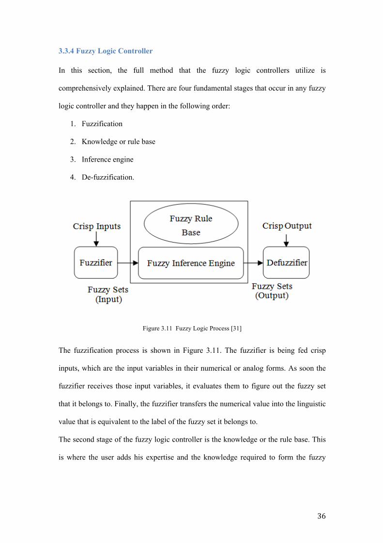
3.3.4 Fuzzy Logic Controller In this section, the full method that the fuzzy logic controllers utilize is
comprehensively explained. There are four fundamental stages that occur in any fuzzy
logic controller and they happen in the following order:
1. Fuzzification
2. Knowledge or rule base
3. Inference engine
4. De-fuzzification.
Figure 3.11 Fuzzy Logic Process [31]
The fuzzification process is shown in Figure 3.11. The fuzzifier is being fed crisp
inputs, which are the input variables in their numerical or analog forms. As soon the
fuzzifier receives those input variables, it evaluates them to figure out the fuzzy set
that it belongs to. Finally, the fuzzifier transfers the numerical value into the linguistic
value that is equivalent to the label of the fuzzy set it belongs to.
The second stage of the fuzzy logic controller is the knowledge or the rule base. This
is where the user adds his expertise and the knowledge required to form the fuzzy
37
rules. Not only does this base translate the user’s experience into the fuzzy rules but
also forms the control goals and policies of the user.
The third stage of the controller is the fuzzy inference engine, which is responsible for
the decision-making action. The fuzzy inference engine receives the input from the
fuzzifier and at the same time extracts the knowledge from the rule base to come up
with an output that matches the users policies. Once a decision has been made and the
engine calculates the output, it then pushes it to the last part of the controller, which is
the de-fuzzifier. The de-fuzzifier, as the name suggests, does the complete opposite of
the fuzzifier. It receives the output from the fuzzy inference engine in the form of a
fuzzy set label and then proceeds to transform this output from linguistic form into
numerical or crisp form [32].
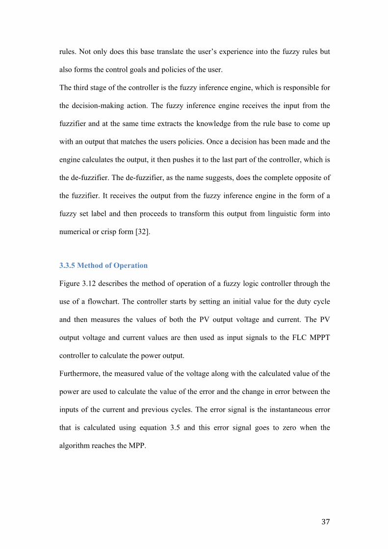
3.3.5 Method of Operation Figure 3.12 describes the method of operation of a fuzzy logic controller through the
use of a flowchart. The controller starts by setting an initial value for the duty cycle
and then measures the values of both the PV output voltage and current. The PV
output voltage and current values are then used as input signals to the FLC MPPT
controller to calculate the power output.
Furthermore, the measured value of the voltage along with the calculated value of the
power are used to calculate the value of the error and the change in error between the
inputs of the current and previous cycles. The error signal is the instantaneous error
that is calculated using equation 3.5 and this error signal goes to zero when the
algorithm reaches the MPP.
38
Figure 3.12 FLC Design Flowchart [33]
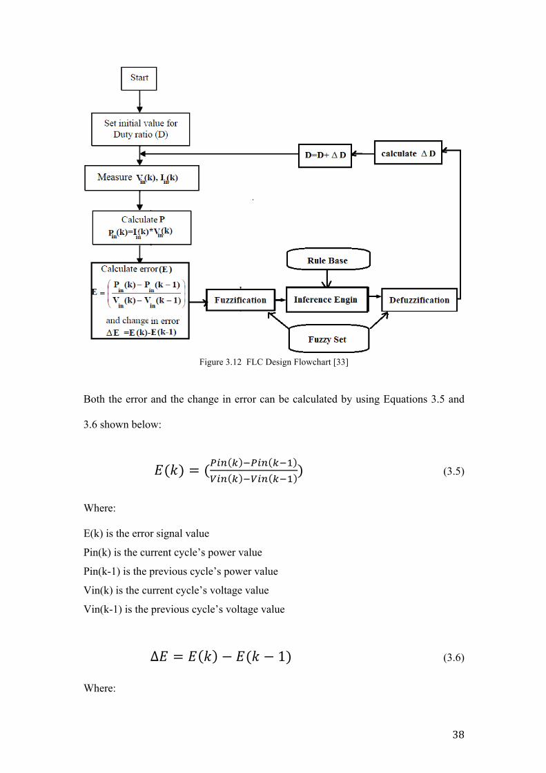
Both the error and the change in error can be calculated by using Equations 3.5 and
3.6 shown below:
𝐸(𝑘) = (!"# ! !!"# !!!!"# ! !!"# !!!
) (3.5)
Where: E(k) is the error signal value
Pin(k) is the current cycle’s power value
Pin(k-1) is the previous cycle’s power value
Vin(k) is the current cycle’s voltage value
Vin(k-1) is the previous cycle’s voltage value
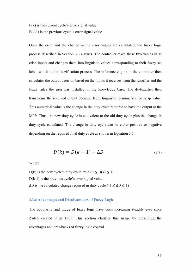
∆𝐸 = 𝐸 𝑘 − 𝐸(𝑘 − 1) (3.6)
Where:
39
E(k) is the current cycle’s error signal value
E(k-1) is the previous cycle’s error signal value
Once the error and the change in the error values are calculated, the fuzzy logic
process described in Section 3.3.4 starts. The controller takes these two values in as
crisp inputs and changes them into linguistic values corresponding to their fuzzy set
label, which is the fuzzification process. The inference engine in the controller then
calculates the output decision based on the inputs it receives from the fuzzifier and the
fuzzy rules the user has installed in the knowledge base. The de-fuzzifier then
transforms the received output decision from linguistic to numerical or crisp value.
This numerical value is the change in the duty cycle required to have the output at the
MPP. Thus, the new duty cycle is equivalent to the old duty cycle plus the change in
duty cycle calculated. The change in duty cycle can be either positive or negative
depending on the required final duty cycle as shown in Equation 3.7:
𝐷(𝑘) = 𝐷 𝑘 − 1 + ∆𝐷 (3.7)
Where: D(k) is the new cycle’s duty cycle ratio (0 ≤ D(k) ≤ 1)
D(k-1) is the previous cycle’s error signal value
∆D is the calculated change required in duty cycle (-1 ≤ ∆D ≤ 1)
3.3.6 Advantages and Disadvantages of Fuzzy Logic
The popularity and usage of fuzzy logic have been increasing steadily ever since
Zadeh created it in 1965. This section clarifies this usage by presenting the
advantages and drawbacks of fuzzy logic control.

40
There are numerous advantages for using fuzzy; however the main one that stands out
is the user-friendly logic. The concept that fuzzy logic was built on was to mimic the
human thinking process, which is why fuzzy logic transforms numbers into language
and the rule base is configured by sentences instead of mathematical equations. Thus,
making it not only much more convenient for the users but also faster to program.
Another major advantage is that unlike other controllers, fuzzy logic has the ability to
work with imprecise mathematical models or ones that are approximated and still
provide an efficient output. Fuzzy logic is consistent and robust even during
frequently fluctuating applications such as the weather condition with solar panels.
Finally, fuzzy logic is capable of working in parallel with other control techniques
such as PID or state feedback [34].
On the other hand, like any other control technique, fuzzy has its drawbacks. Firstly,
compared to P&O and INC, FLC is much more complex. The former two techniques
require the usage of one or more sensors and thus they are simpler to use. Moreover,
higher complexity translates into higher cost of implementation. Another drawback is
when an accurate mathematical model of a complex project is available; it tends to be
easier and quicker to use a controller that utilizes this model instead of re-writing the
model to conditional statements. In this case fuzzy would not be the optimum choice.
41
Chapter 4 Design & Analysis
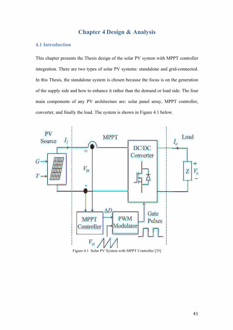
4.1 Introduction This chapter presents the Thesis design of the solar PV system with MPPT controller
integration. There are two types of solar PV systems: standalone and grid-connected.
In this Thesis, the standalone system is chosen because the focus is on the generation
of the supply side and how to enhance it rather than the demand or load side. The four
main components of any PV architecture are: solar panel array, MPPT controller,
converter, and finally the load. The system is shown in Figure 4.1 below.
Figure 4.1 Solar PV System with MPPT Controller [35]
42
4.2 System Architecture
Figure 4.2 PV Solar System Design on MATLAB (Adapted from [36])

43
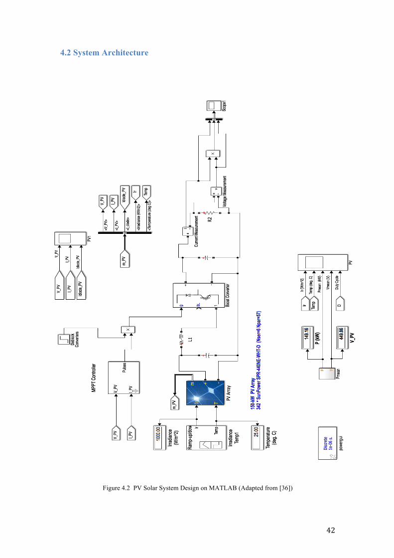
Figure 4.2 shows the architecture of the PV solar system designed for this thesis. This
design is common for the three algorithms except for the MPPT controller block,
where it differs for each of the algorithms in use. The three algorithms are: Perturb &
Observe (P&O), Incremental Conductance with Integral regulator (INC), and finally
Fuzzy Logic.
Figure 4.2 shows the components of the system, which are:
- PV Array (Model: Sun Power SPR- 440NE-WHT-D, 6S and 57P)
- MPPT Controller
- Boost Converter
- 2 Capacitors
- 2 Resistors
- 1 Inductor
The PV system design starts with a Ramp-up/ down module that controls and
fluctuates the value of the temperature and the irradiance to simulate real life
conditions. These values are being fed to the PV array block, which outputs a certain
voltage and current depending on the specific values of the temperature and
irradiance. The voltage and current values taken from the PV array are used as inputs
to the MPPT controller while the output of the array is connected to a DC-DC Boost
converter. The MPPT controller uses the input PV voltage and current value to
continuously calculate the duty cycle, which is then fed to the boost converter. The
boos converter controls the voltage level according to the duty cycle to keep tracking
the Maximum Power Point at all times. Finally, the output of the boost converter is
then connected to a resistive load, which acts as a demand side load for the stand-
alone system.
44
4.2.1 Photovoltaic Module There are various PV technology types including mono-crystalline silicon cells, multi-
crystalline silicon cells, and amorphous silicon cells. The type chosen in this Thesis is
the mono-crystalline silicon cell for their high efficiency. The solar panel that was
chosen in this design is the Sun Power SPR- 440NE-WHT-D. Sun Power is a well-
known manufacturer of solar panels and among the best in the market when it comes
to a solar panel’s performance.
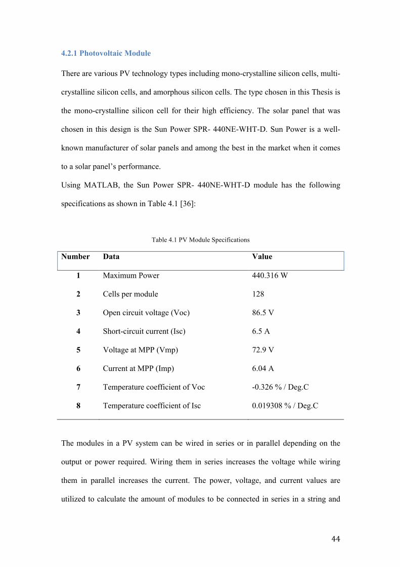
Using MATLAB, the Sun Power SPR- 440NE-WHT-D module has the following
specifications as shown in Table 4.1 [36]:
Table 4.1 PV Module Specifications
Number Data Value
1 Maximum Power 440.316 W
2 Cells per module 128
3 Open circuit voltage (Voc) 86.5 V
4 Short-circuit current (Isc) 6.5 A
5 Voltage at MPP (Vmp) 72.9 V
6 Current at MPP (Imp) 6.04 A
7 Temperature coefficient of Voc -0.326 % / Deg.C
8 Temperature coefficient of Isc 0.019308 % / Deg.C
The modules in a PV system can be wired in series or in parallel depending on the
output or power required. Wiring them in series increases the voltage while wiring
them in parallel increases the current. The power, voltage, and current values are
utilized to calculate the amount of modules to be connected in series in a string and
45
how many parallel strings are needed to reach the targeted output power. Therefore,
using the values given in Table 4.1, the design has to have six modules connected in
series in a string and 57 parallel strings to reach the required output power, which is
150 kW.
4.2.2 MPPT
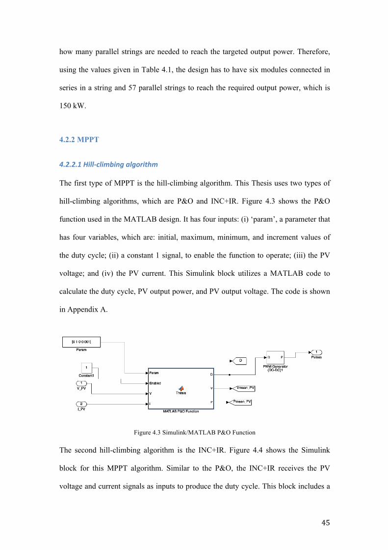
4.2.2.1Hill-climbingalgorithmThe first type of MPPT is the hill-climbing algorithm. This Thesis uses two types of
hill-climbing algorithms, which are P&O and INC+IR. Figure 4.3 shows the P&O
function used in the MATLAB design. It has four inputs: (i) ‘param’, a parameter that
has four variables, which are: initial, maximum, minimum, and increment values of
the duty cycle; (ii) a constant 1 signal, to enable the function to operate; (iii) the PV
voltage; and (iv) the PV current. This Simulink block utilizes a MATLAB code to
calculate the duty cycle, PV output power, and PV output voltage. The code is shown
in Appendix A.
Figure 4.3 Simulink/MATLAB P&O Function
The second hill-climbing algorithm is the INC+IR. Figure 4.4 shows the Simulink
block for this MPPT algorithm. Similar to the P&O, the INC+IR receives the PV
voltage and current signals as inputs to produce the duty cycle. This block includes a
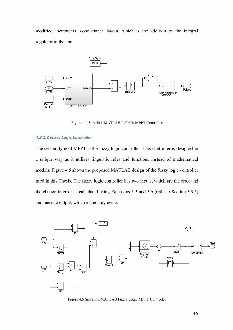
46
modified incremental conductance layout, which is the addition of the integral
regulator in the end.
Figure 4.4 Simulink/MATLAB INC+IR MPPT Controller
4.2.2.2FuzzyLogicControllerThe second type of MPPT is the fuzzy logic controller. This controller is designed in
a unique way as it utilizes linguistic rules and functions instead of mathematical
models. Figure 4.5 shows the proposed MATLAB design of the fuzzy logic controller
used in this Thesis. The fuzzy logic controller has two inputs, which are the error and
the change in error as calculated using Equations 3.5 and 3.6 (refer to Section 3.3.5)
and has one output, which is the duty cycle.
Figure 4.5 Simulink/MATLAB Fuzzy Logic MPPT Controller
47
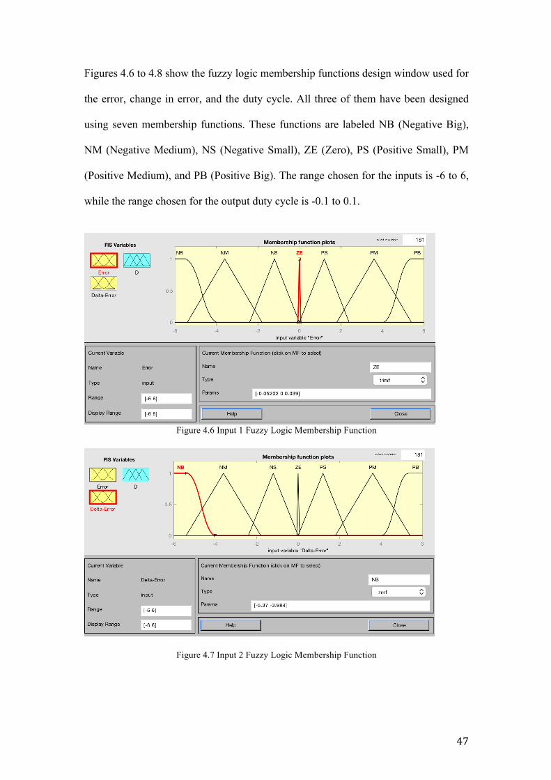
Figures 4.6 to 4.8 show the fuzzy logic membership functions design window used for
the error, change in error, and the duty cycle. All three of them have been designed
using seven membership functions. These functions are labeled NB (Negative Big),
NM (Negative Medium), NS (Negative Small), ZE (Zero), PS (Positive Small), PM
(Positive Medium), and PB (Positive Big). The range chosen for the inputs is -6 to 6,
while the range chosen for the output duty cycle is -0.1 to 0.1.
Figure 4.6 Input 1 Fuzzy Logic Membership Function
Figure 4.7 Input 2 Fuzzy Logic Membership Function
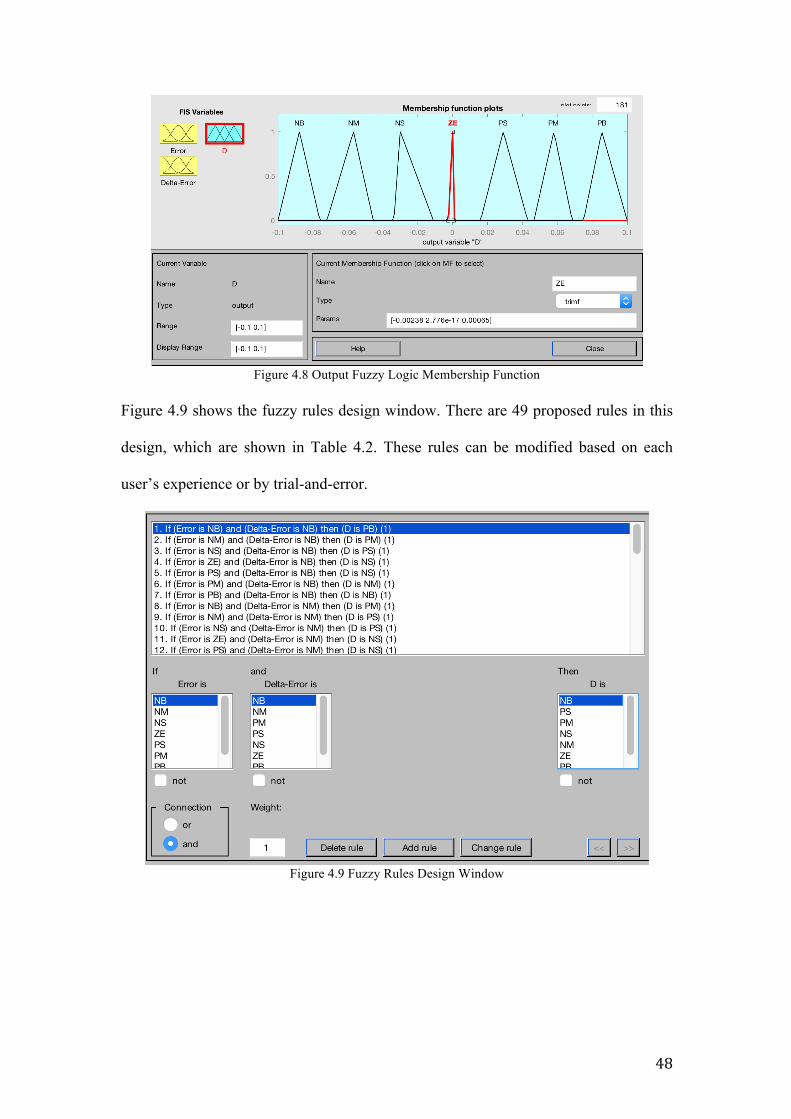
48
Figure 4.8 Output Fuzzy Logic Membership Function
Figure 4.9 shows the fuzzy rules design window. There are 49 proposed rules in this
design, which are shown in Table 4.2. These rules can be modified based on each
user’s experience or by trial-and-error.
Figure 4.9 Fuzzy Rules Design Window
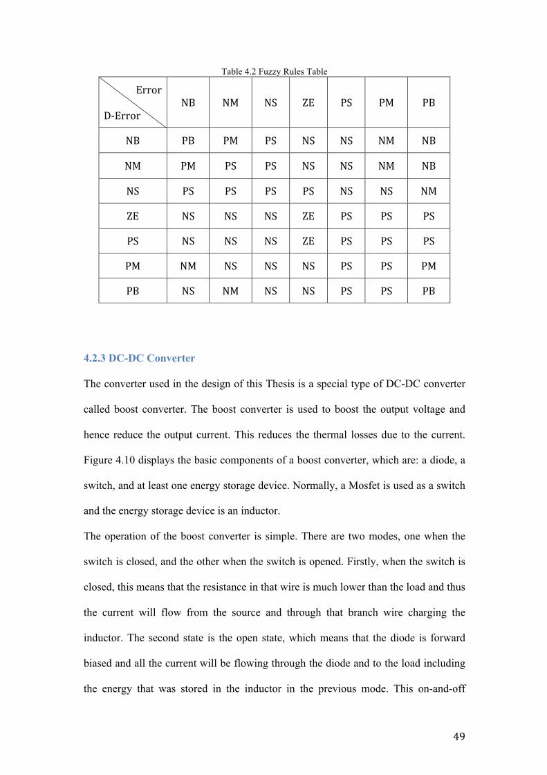
49
Table 4.2 Fuzzy Rules Table
Error
D-ErrorNB NM NS ZE PS PM PB
NB PB PM PS NS NS NM NB
NM PM PS PS NS NS NM NB
NS PS PS PS PS NS NS NM
ZE NS NS NS ZE PS PS PS
PS NS NS NS ZE PS PS PS
PM NM NS NS NS PS PS PM
PB NS NM NS NS PS PS PB
4.2.3 DC-DC Converter The converter used in the design of this Thesis is a special type of DC-DC converter
called boost converter. The boost converter is used to boost the output voltage and
hence reduce the output current. This reduces the thermal losses due to the current.
Figure 4.10 displays the basic components of a boost converter, which are: a diode, a
switch, and at least one energy storage device. Normally, a Mosfet is used as a switch
and the energy storage device is an inductor.
The operation of the boost converter is simple. There are two modes, one when the
switch is closed, and the other when the switch is opened. Firstly, when the switch is
closed, this means that the resistance in that wire is much lower than the load and thus
the current will flow from the source and through that branch wire charging the
inductor. The second state is the open state, which means that the diode is forward
biased and all the current will be flowing through the diode and to the load including
the energy that was stored in the inductor in the previous mode. This on-and-off
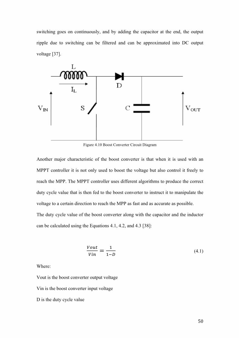
50
switching goes on continuously, and by adding the capacitor at the end, the output
ripple due to switching can be filtered and can be approximated into DC output
voltage [37].
Figure 4.10 Boost Converter Circuit Diagram
Another major characteristic of the boost converter is that when it is used with an
MPPT controller it is not only used to boost the voltage but also control it freely to
reach the MPP. The MPPT controller uses different algorithms to produce the correct
duty cycle value that is then fed to the boost converter to instruct it to manipulate the
voltage to a certain direction to reach the MPP as fast and as accurate as possible.
The duty cycle value of the boost converter along with the capacitor and the inductor
can be calculated using the Equations 4.1, 4.2, and 4.3 [38]:
!"#$!"#
= !!!!
(4.1)
Where:
Vout is the boost converter output voltage
Vin is the boost converter input voltage
D is the duty cycle value
51
Moreover, both the inductor and capacitor in the model can be designed using
Equations 4.2 and 4.3:
𝐿 = !"#∗!"#∆!𝐿
(4.2)
Where:
L is the minimum value of the inductor
Vin is the boost converter input voltage
Ton is the turn on time of the transistor
∆IL is the desired change in current ripple
𝐶 = !𝑙𝑜𝑎𝑑∗!"#∆!𝑐
(4.3)
Where:
C is the value of the capacitor
Iload is the current going through the load
Ton is the turn on time of the transistor
∆Vc is the desired change in voltage ripple
4.3 Effect of Temperature and Irradiance on the PV Output Power There are several factors that affect the output of the PV system. Among these factors
are: geographic location, meteorological conditions (such as amount of sunlight and
snow), shading, dust and debris, irradiance, and temperature. Although all these
factors have an effect on the output of the PV, the main factors that affect the
operating conditions are the irradiance hitting the surface of the solar panel and the
temperature of the panel itself.
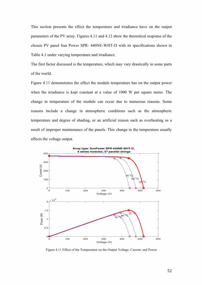
52
This section presents the effect the temperature and irradiance have on the output
parameters of the PV array. Figures 4.11 and 4.12 show the theoretical response of the
chosen PV panel Sun Power SPR- 440NE-WHT-D with its specifications shown in
Table 4.1 under varying temperature and irradiance.
The first factor discussed is the temperature, which may vary drastically in some parts
of the world.
Figure 4.11 demonstrates the effect the module temperature has on the output power
when the irradiance is kept constant at a value of 1000 W per square meter. The
change in temperature of the module can occur due to numerous reasons. Some
reasons include a change in atmospheric conditions such as the atmospheric
temperature and degree of shading, or an artificial reason such as overheating as a
result of improper maintenance of the panels. This change in the temperature usually
affects the voltage output.
Figure 4.11 Effect of the Temperature on the Output Voltage, Current, and Power
0 100 200 300 400 500 600Voltage (V)
0
100
200
300
400
Curre
nt (A
)
Array type: SunPower SPR-440NE-WHT-D;6 series modules; 57 parallel strings
25 oC50 oC
70 oC
0 100 200 300 400 500 600Voltage (V)
0
0.5
1
1.5
2
Powe
r (W
)
105
25 oC50 oC
70 oC
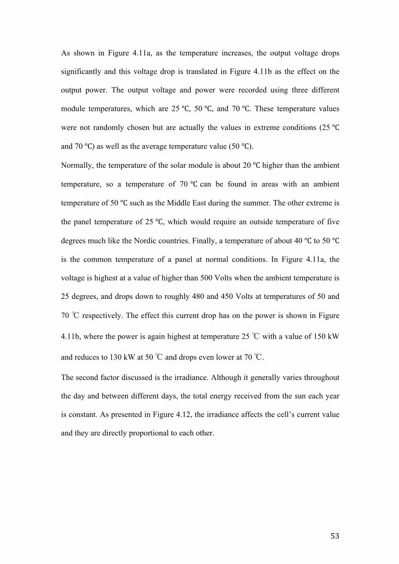
53
As shown in Figure 4.11a, as the temperature increases, the output voltage drops
significantly and this voltage drop is translated in Figure 4.11b as the effect on the
output power. The output voltage and power were recorded using three different
module temperatures, which are 25 ℃, 50 ℃, and 70 ℃. These temperature values
were not randomly chosen but are actually the values in extreme conditions (25 ℃
and 70 ℃) as well as the average temperature value (50 ℃).
Normally, the temperature of the solar module is about 20 ℃ higher than the ambient
temperature, so a temperature of 70 ℃ can be found in areas with an ambient
temperature of 50 ℃ such as the Middle East during the summer. The other extreme is
the panel temperature of 25 ℃, which would require an outside temperature of five
degrees much like the Nordic countries. Finally, a temperature of about 40 ℃ to 50 ℃
is the common temperature of a panel at normal conditions. In Figure 4.11a, the
voltage is highest at a value of higher than 500 Volts when the ambient temperature is
25 degrees, and drops down to roughly 480 and 450 Volts at temperatures of 50 and
70 ℃ respectively. The effect this current drop has on the power is shown in Figure
4.11b, where the power is again highest at temperature 25 ℃ with a value of 150 kW
and reduces to 130 kW at 50 ℃ and drops even lower at 70 ℃.
The second factor discussed is the irradiance. Although it generally varies throughout
the day and between different days, the total energy received from the sun each year
is constant. As presented in Figure 4.12, the irradiance affects the cell’s current value
and they are directly proportional to each other.
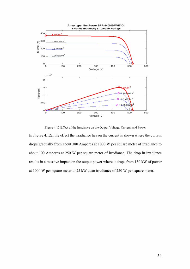
54
Figure 4.12 Effect of the Irradiance on the Output Voltage, Current, and Power
In Figure 4.12a, the effect the irradiance has on the current is shown where the current
drops gradually from about 380 Amperes at 1000 W per square meter of irradiance to
about 100 Amperes at 250 W per square meter of irradiance. The drop in irradiance
results in a massive impact on the output power where it drops from 150 kW of power
at 1000 W per square meter to 25 kW at an irradiance of 250 W per square meter.
0 100 200 300 400 500 600Voltage (V)
0
100
200
300
400
Curre
nt (A
)
Array type: SunPower SPR-440NE-WHT-D;6 series modules; 57 parallel strings
1 kW/m2
0.75 kW/m2
0.5 kW/m2
0.25 kW/m2
0 100 200 300 400 500 600Voltage (V)
0
0.5
1
1.5
2
Powe
r (W
)
105
1 kW/m2
0.75 kW/m2
0.5 kW/m2
0.25 kW/m2
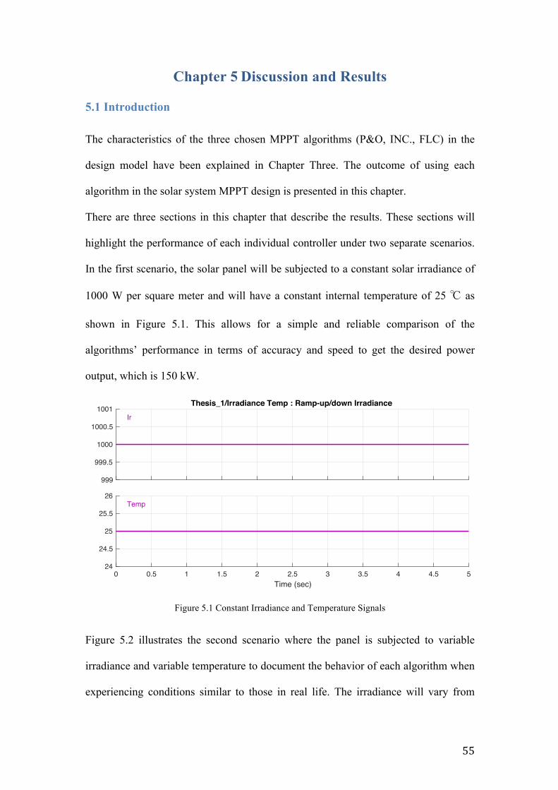
55
Chapter 5 Discussion and Results
5.1 Introduction The characteristics of the three chosen MPPT algorithms (P&O, INC., FLC) in the
design model have been explained in Chapter Three. The outcome of using each
algorithm in the solar system MPPT design is presented in this chapter.
There are three sections in this chapter that describe the results. These sections will
highlight the performance of each individual controller under two separate scenarios.
In the first scenario, the solar panel will be subjected to a constant solar irradiance of
1000 W per square meter and will have a constant internal temperature of 25 ℃ as
shown in Figure 5.1. This allows for a simple and reliable comparison of the
algorithms’ performance in terms of accuracy and speed to get the desired power
output, which is 150 kW.
Figure 5.1 Constant Irradiance and Temperature Signals
Figure 5.2 illustrates the second scenario where the panel is subjected to variable
irradiance and variable temperature to document the behavior of each algorithm when
experiencing conditions similar to those in real life. The irradiance will vary from
999
999.5
1000
1000.5
1001Thesis_1/Irradiance Temp : Ramp-up/down Irradiance
Ir
0 0.5 1 1.5 2 2.5 3 3.5 4 4.5 5Time (sec)
24
24.5
25
25.5
26Temp
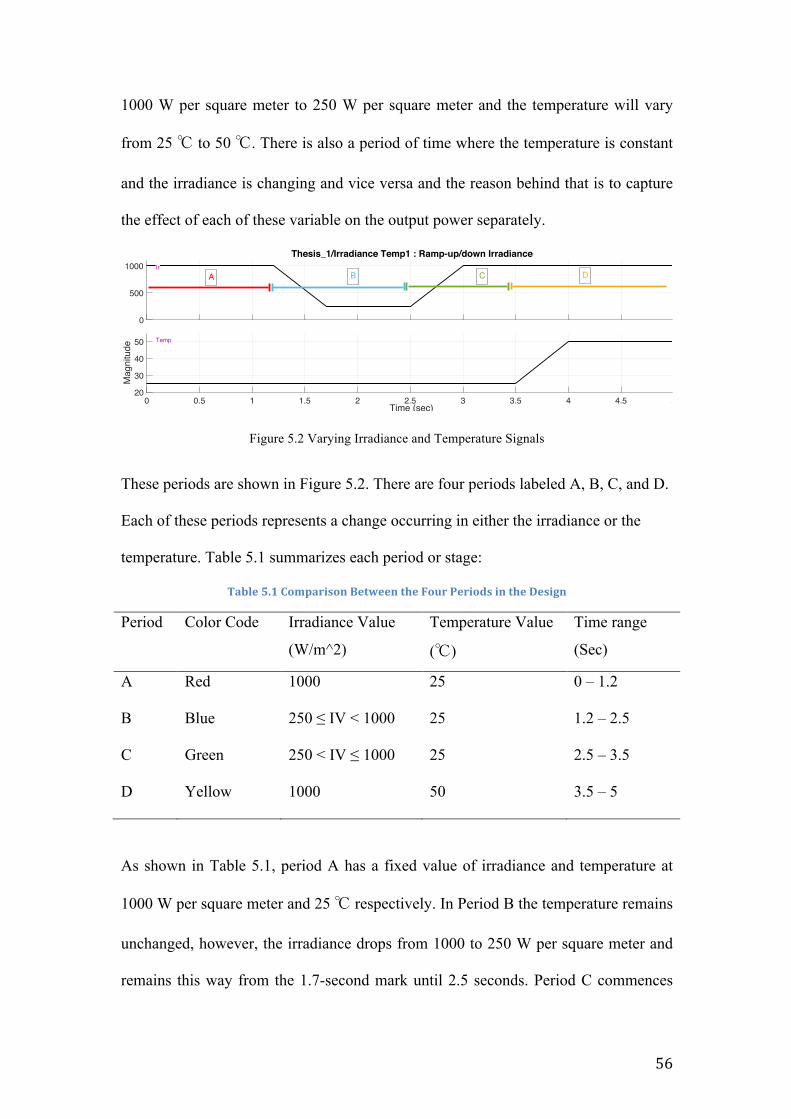
56
1000 W per square meter to 250 W per square meter and the temperature will vary
from 25 ℃ to 50 ℃. There is also a period of time where the temperature is constant
and the irradiance is changing and vice versa and the reason behind that is to capture
the effect of each of these variable on the output power separately.
Figure 5.2 Varying Irradiance and Temperature Signals
These periods are shown in Figure 5.2. There are four periods labeled A, B, C, and D.
Each of these periods represents a change occurring in either the irradiance or the
temperature. Table 5.1 summarizes each period or stage:
Table5.1ComparisonBetweentheFourPeriodsintheDesign
Period Color Code Irradiance Value
(W/m^2)
Temperature Value
(℃)
Time range
(Sec)
A Red 1000 25 0 – 1.2
B Blue 250 ≤ IV < 1000 25 1.2 – 2.5
C Green 250 < IV ≤ 1000 25 2.5 – 3.5
D Yellow 1000 50 3.5 – 5
As shown in Table 5.1, period A has a fixed value of irradiance and temperature at
1000 W per square meter and 25 ℃ respectively. In Period B the temperature remains
unchanged, however, the irradiance drops from 1000 to 250 W per square meter and
remains this way from the 1.7-second mark until 2.5 seconds. Period C commences
0
500
1000Thesis_1/Irradiance Temp1 : Ramp-up/down Irradiance
Ir
0 0.5 1 1.5 2 2.5 3 3.5 4 4.5 5Time (sec)
20
30
40
50
Mag
nitu
de
Temp
A B C D
57
after the 2.5 second mark, increasing the voltage back to 1000 W per square meter.
Finally, in period D, the first change in the temperature is witnesses from 25 ℃ to 50
℃ while having an irradiance of 1000 W per square meter.
Sections 5.2, 5.3, and 5.4 contain two scenarios. In order to evaluate the results, each
of these scenarios will contain the following three graphs:
- Change in Solar Irradiance and Ambient Temperature Versus Time
- System Output Power, Voltage, and Current Versus Time
- Duty Cycle, PV Voltage and Current, and System Output Voltage and
Current Versus Time.
5.2 Perturb & Observe Algorithm Results
5.2.1 Scenario One: Constant Irradiance and Temperature This section describes the simulation of the PV MPPT system under constant solar
irradiance and module temperature where the irradiance is kept constant at 1000 W
per square meter and the temperature at 25 ℃ (refer to Figure 5.1). When both
variables are kept constant, the result will be as shown in Figure 5.3. The plot shows
three lines using different color codes. As shown in the legend, blue is for the output
power, red is for the output voltage, and finally, yellow is the output current.
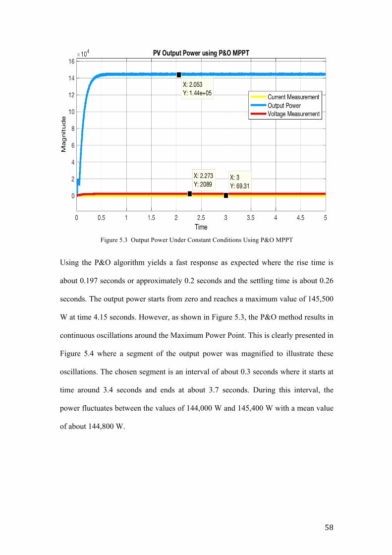
58
Figure 5.3 Output Power Under Constant Conditions Using P&O MPPT
Using the P&O algorithm yields a fast response as expected where the rise time is
about 0.197 seconds or approximately 0.2 seconds and the settling time is about 0.26
seconds. The output power starts from zero and reaches a maximum value of 145,500
W at time 4.15 seconds. However, as shown in Figure 5.3, the P&O method results in
continuous oscillations around the Maximum Power Point. This is clearly presented in
Figure 5.4 where a segment of the output power was magnified to illustrate these
oscillations. The chosen segment is an interval of about 0.3 seconds where it starts at
time around 3.4 seconds and ends at about 3.7 seconds. During this interval, the
power fluctuates between the values of 144,000 W and 145,400 W with a mean value
of about 144,800 W.
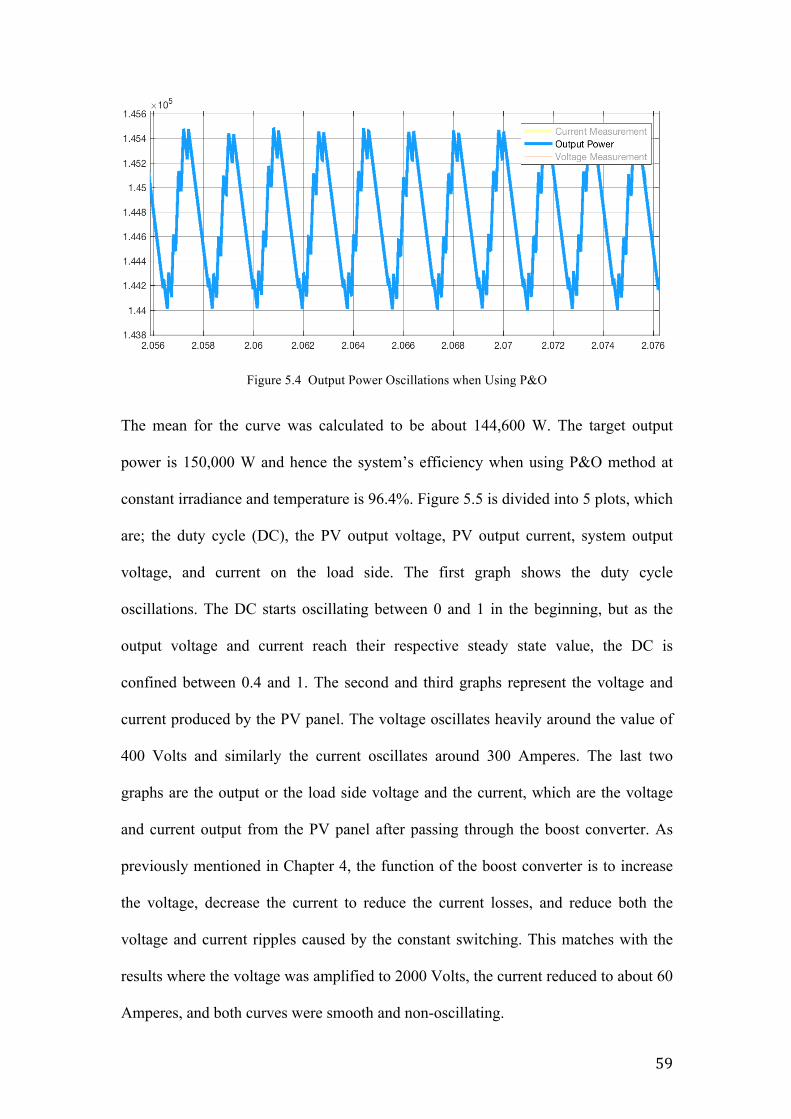
59
Figure 5.4 Output Power Oscillations when Using P&O
The mean for the curve was calculated to be about 144,600 W. The target output
power is 150,000 W and hence the system’s efficiency when using P&O method at
constant irradiance and temperature is 96.4%. Figure 5.5 is divided into 5 plots, which
are; the duty cycle (DC), the PV output voltage, PV output current, system output
voltage, and current on the load side. The first graph shows the duty cycle
oscillations. The DC starts oscillating between 0 and 1 in the beginning, but as the
output voltage and current reach their respective steady state value, the DC is
confined between 0.4 and 1. The second and third graphs represent the voltage and
current produced by the PV panel. The voltage oscillates heavily around the value of
400 Volts and similarly the current oscillates around 300 Amperes. The last two
graphs are the output or the load side voltage and the current, which are the voltage
and current output from the PV panel after passing through the boost converter. As
previously mentioned in Chapter 4, the function of the boost converter is to increase
the voltage, decrease the current to reduce the current losses, and reduce both the
voltage and current ripples caused by the constant switching. This matches with the
results where the voltage was amplified to 2000 Volts, the current reduced to about 60
Amperes, and both curves were smooth and non-oscillating.
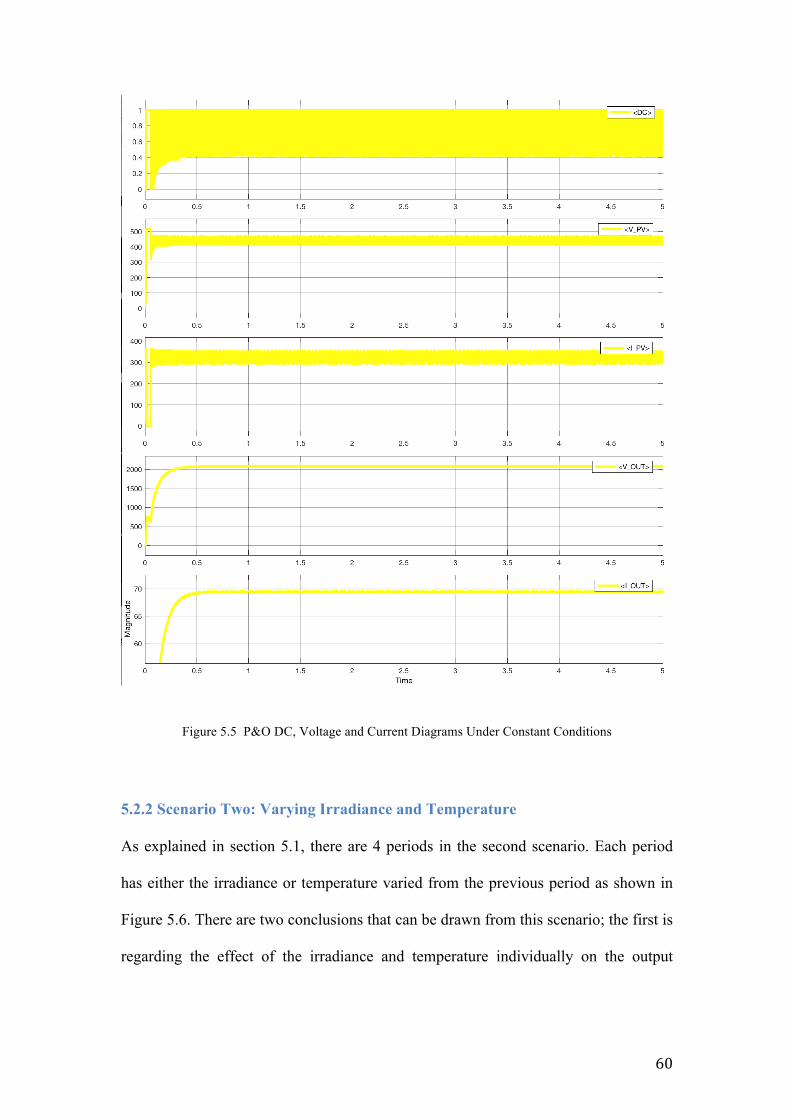
60
Figure 5.5 P&O DC, Voltage and Current Diagrams Under Constant Conditions
5.2.2 Scenario Two: Varying Irradiance and Temperature As explained in section 5.1, there are 4 periods in the second scenario. Each period
has either the irradiance or temperature varied from the previous period as shown in
Figure 5.6. There are two conclusions that can be drawn from this scenario; the first is
regarding the effect of the irradiance and temperature individually on the output
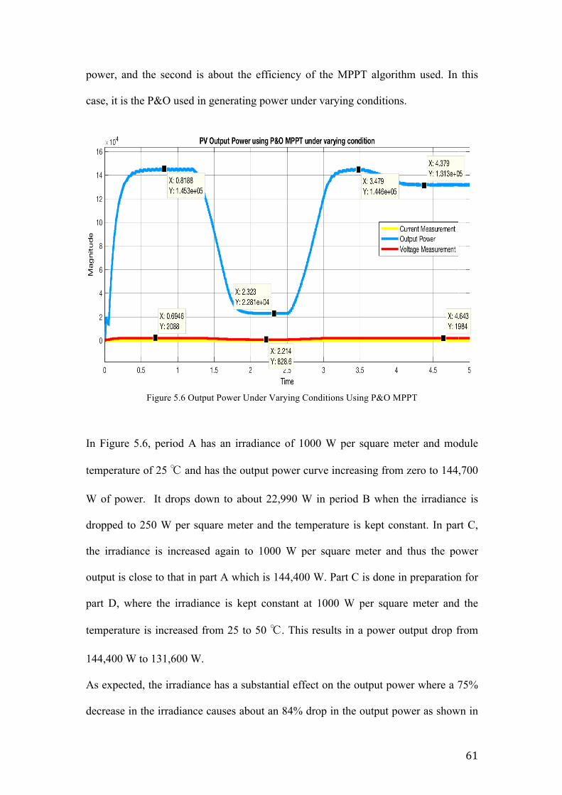
61
power, and the second is about the efficiency of the MPPT algorithm used. In this
case, it is the P&O used in generating power under varying conditions.
Figure 5.6 Output Power Under Varying Conditions Using P&O MPPT
In Figure 5.6, period A has an irradiance of 1000 W per square meter and module
temperature of 25 ℃ and has the output power curve increasing from zero to 144,700
W of power. It drops down to about 22,990 W in period B when the irradiance is
dropped to 250 W per square meter and the temperature is kept constant. In part C,
the irradiance is increased again to 1000 W per square meter and thus the power
output is close to that in part A which is 144,400 W. Part C is done in preparation for
part D, where the irradiance is kept constant at 1000 W per square meter and the
temperature is increased from 25 to 50 ℃. This results in a power output drop from
144,400 W to 131,600 W.
As expected, the irradiance has a substantial effect on the output power where a 75%
decrease in the irradiance causes about an 84% drop in the output power as shown in
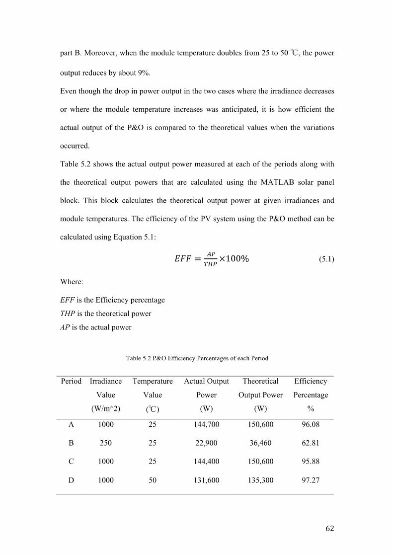
62
part B. Moreover, when the module temperature doubles from 25 to 50 ℃, the power
output reduces by about 9%.
Even though the drop in power output in the two cases where the irradiance decreases
or where the module temperature increases was anticipated, it is how efficient the
actual output of the P&O is compared to the theoretical values when the variations
occurred.
Table 5.2 shows the actual output power measured at each of the periods along with
the theoretical output powers that are calculated using the MATLAB solar panel
block. This block calculates the theoretical output power at given irradiances and
module temperatures. The efficiency of the PV system using the P&O method can be
calculated using Equation 5.1:
𝐸𝐹𝐹 = !"!"#
×100% (5.1)
Where:
EFF is the Efficiency percentage
THP is the theoretical power
AP is the actual power
Table 5.2 P&O Efficiency Percentages of each Period
Period Irradiance
Value
(W/m^2)
Temperature
Value
(℃)
Actual Output
Power
(W)
Theoretical
Output Power
(W)
Efficiency
Percentage
%
A 1000 25 144,700 150,600 96.08
B 250 25 22,900 36,460 62.81
C 1000 25 144,400 150,600 95.88
D 1000 50 131,600 135,300 97.27
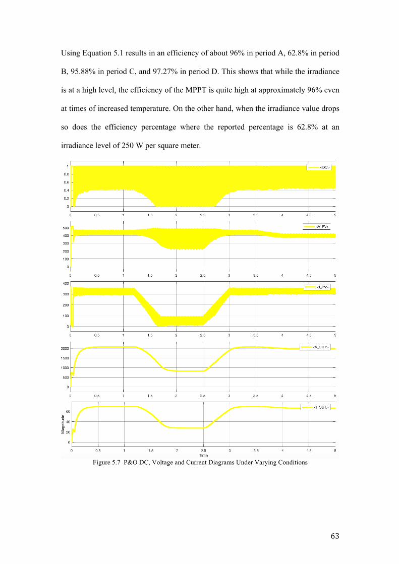
63
Using Equation 5.1 results in an efficiency of about 96% in period A, 62.8% in period
B, 95.88% in period C, and 97.27% in period D. This shows that while the irradiance
is at a high level, the efficiency of the MPPT is quite high at approximately 96% even
at times of increased temperature. On the other hand, when the irradiance value drops
so does the efficiency percentage where the reported percentage is 62.8% at an
irradiance level of 250 W per square meter.
Figure 5.7 P&O DC, Voltage and Current Diagrams Under Varying Conditions
64
The last part of this scenario (and section) is Figure 5.7. This figure shows the duty
cycle values, PV output voltage and current, and the system output voltage and
current. Similar to the first scenario, the PV output voltage and current oscillate
heavily until they pass through the boost converter, which allows for a boost in
voltage, a drop in current, and removing the oscillations from both curves. Moreover,
an observation in the PV voltage and current curves is that while a decrease in
irradiance affects both these variables as shown in period B, the PV current is affected
more. The current drops from an average of 320 Amperes to an average of 80
Amperes, while the voltage only drops from an average of 450 Volts to about 350
Volts. On the other hand, an increase in the temperature affects the PV voltage where
it drops from 450 Volts to about 400 Volts; however, the temperature spike from 25
℃ to 50 ℃ has an insignificant effect on the current that does not manifest on the
curve. Finally, the voltage and current of the output system seem to react in a similar
manner where they are both affected similarly during the drop in irradiance and rise in
temperature. The output voltage starts at 2100 Volts in period A, drops to about 850
Volts in period B, goes back up to 2100 Volts in period C and finally reduces a bit
more to 2000 Volts in period D. Likewise, the output current starts at 70 Amperes,
drops to 28 Amperes, back to 68 Amperes, and finally reduces to about 66 Amperes.
5.3 Incremental Conductance +Integral Regulator This section is dedicated towards presenting the results of using the incremental
conductance algorithm with an integral regulator as a Maximum Power Point Tracker.
5.3.1 Scenario One: Constant Irradiance and Temperature
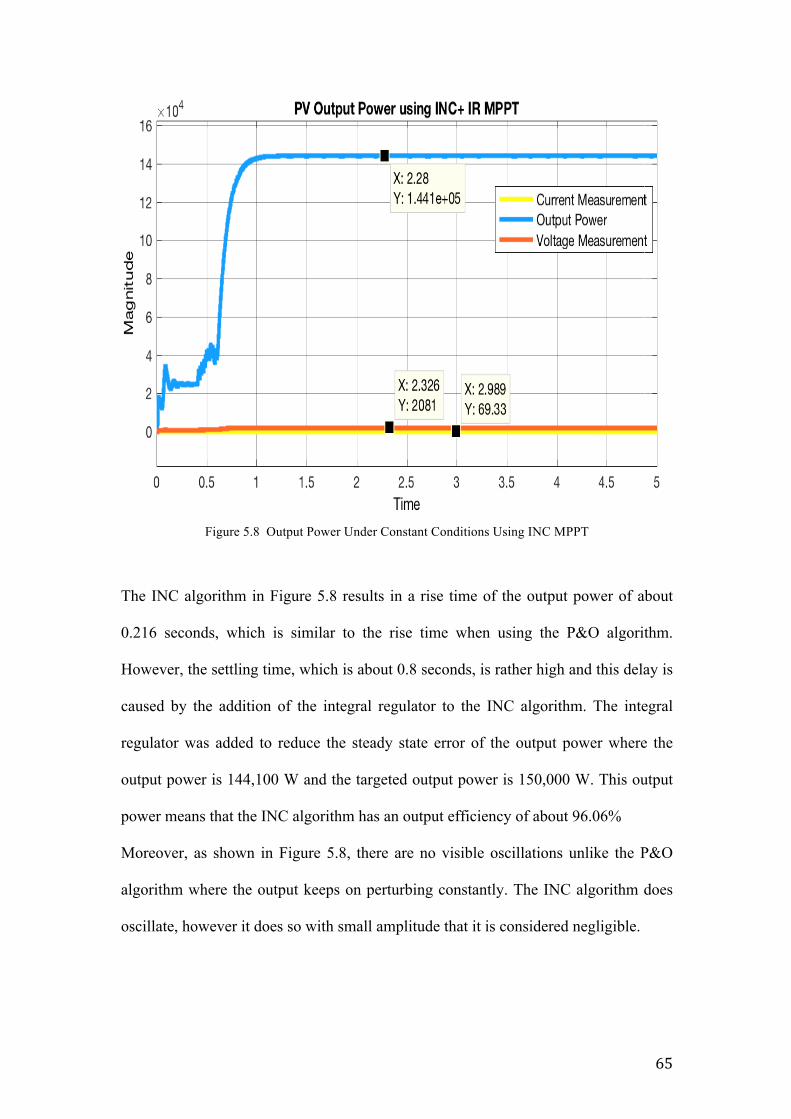
65
Figure 5.8 Output Power Under Constant Conditions Using INC MPPT
The INC algorithm in Figure 5.8 results in a rise time of the output power of about
0.216 seconds, which is similar to the rise time when using the P&O algorithm.
However, the settling time, which is about 0.8 seconds, is rather high and this delay is
caused by the addition of the integral regulator to the INC algorithm. The integral
regulator was added to reduce the steady state error of the output power where the
output power is 144,100 W and the targeted output power is 150,000 W. This output
power means that the INC algorithm has an output efficiency of about 96.06%
Moreover, as shown in Figure 5.8, there are no visible oscillations unlike the P&O
algorithm where the output keeps on perturbing constantly. The INC algorithm does
oscillate, however it does so with small amplitude that it is considered negligible.
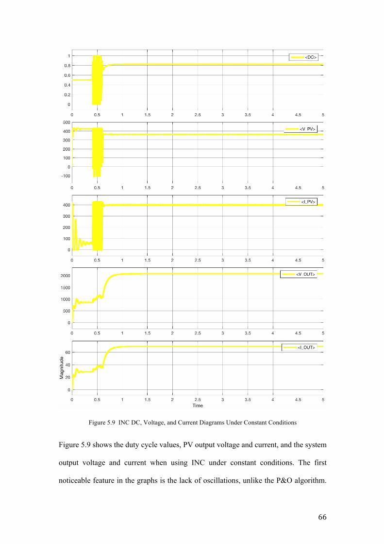
66
Figure 5.9 INC DC, Voltage, and Current Diagrams Under Constant Conditions
Figure 5.9 shows the duty cycle values, PV output voltage and current, and the system
output voltage and current when using INC under constant conditions. The first
noticeable feature in the graphs is the lack of oscillations, unlike the P&O algorithm.
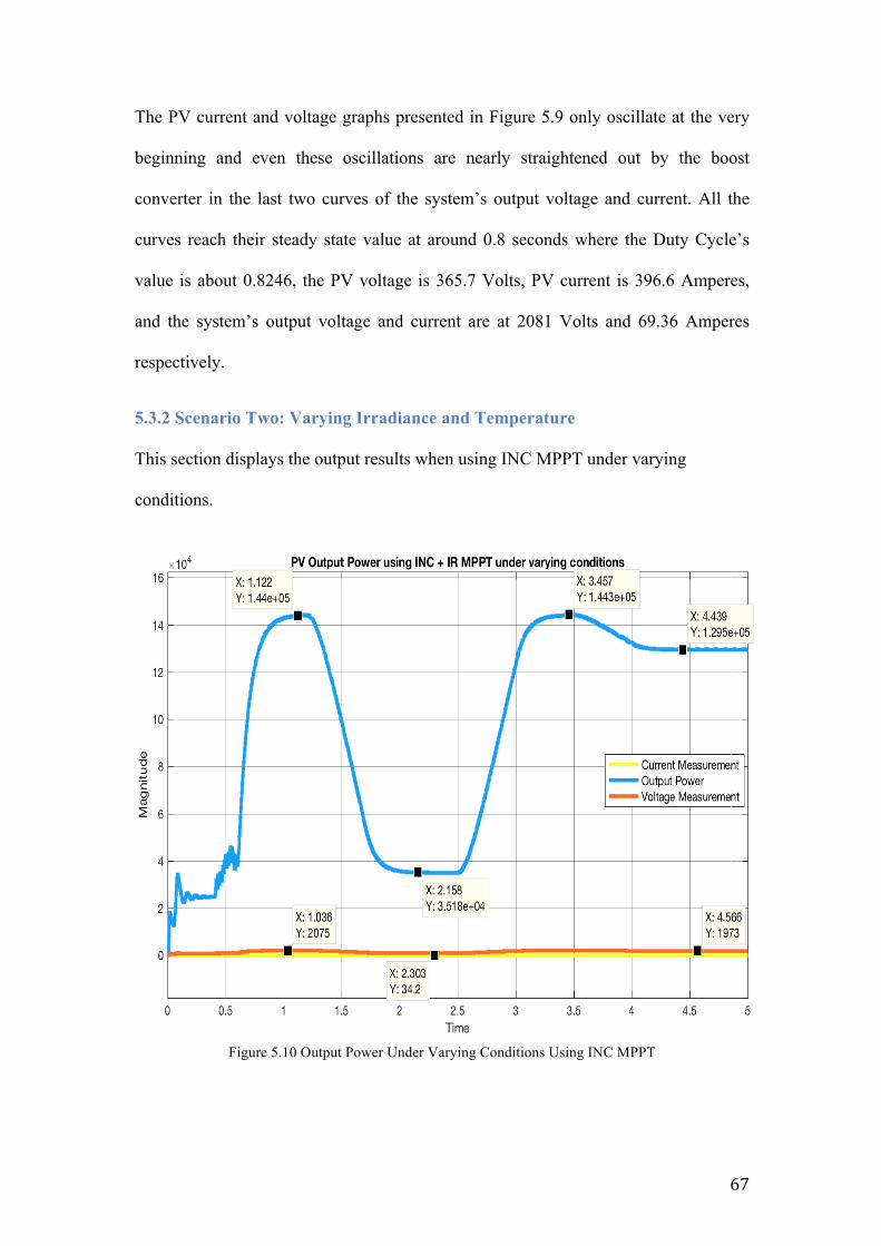
67
The PV current and voltage graphs presented in Figure 5.9 only oscillate at the very
beginning and even these oscillations are nearly straightened out by the boost
converter in the last two curves of the system’s output voltage and current. All the
curves reach their steady state value at around 0.8 seconds where the Duty Cycle’s
value is about 0.8246, the PV voltage is 365.7 Volts, PV current is 396.6 Amperes,
and the system’s output voltage and current are at 2081 Volts and 69.36 Amperes
respectively.
5.3.2 Scenario Two: Varying Irradiance and Temperature This section displays the output results when using INC MPPT under varying
conditions.
Figure 5.10 Output Power Under Varying Conditions Using INC MPPT
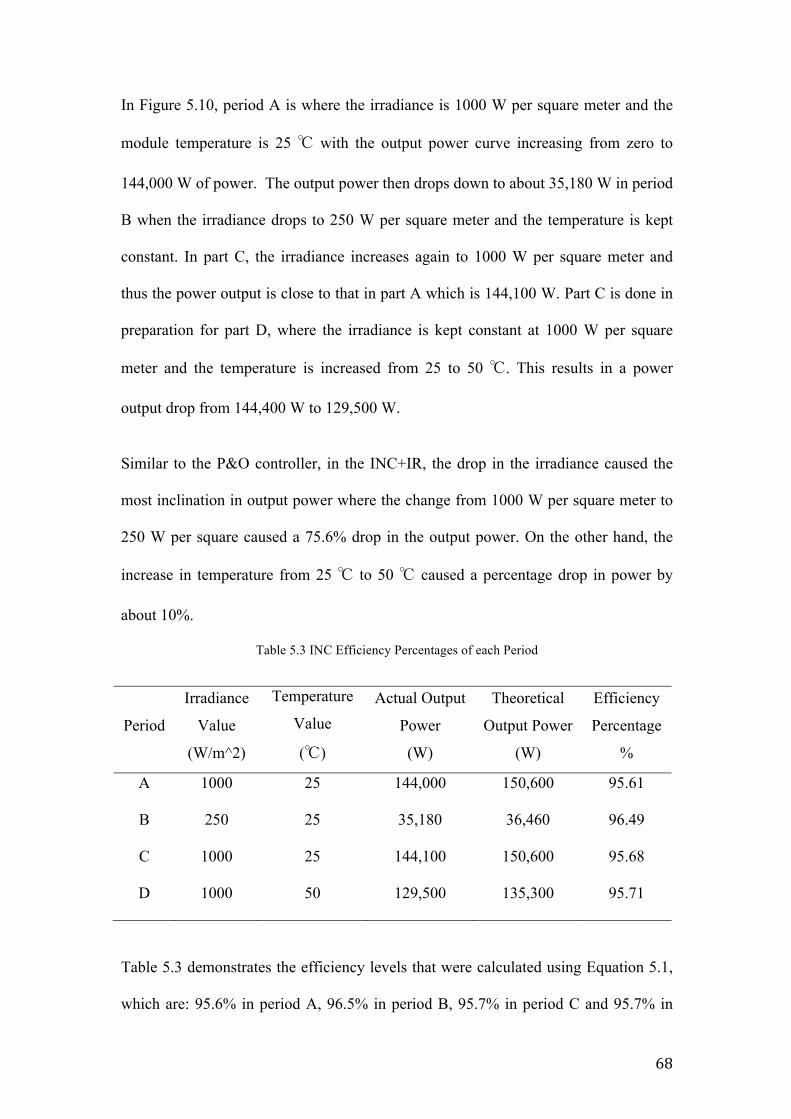
68
In Figure 5.10, period A is where the irradiance is 1000 W per square meter and the
module temperature is 25 ℃ with the output power curve increasing from zero to
144,000 W of power. The output power then drops down to about 35,180 W in period
B when the irradiance drops to 250 W per square meter and the temperature is kept
constant. In part C, the irradiance increases again to 1000 W per square meter and
thus the power output is close to that in part A which is 144,100 W. Part C is done in
preparation for part D, where the irradiance is kept constant at 1000 W per square
meter and the temperature is increased from 25 to 50 ℃. This results in a power
output drop from 144,400 W to 129,500 W.
Similar to the P&O controller, in the INC+IR, the drop in the irradiance caused the
most inclination in output power where the change from 1000 W per square meter to
250 W per square caused a 75.6% drop in the output power. On the other hand, the
increase in temperature from 25 ℃ to 50 ℃ caused a percentage drop in power by
about 10%.
Table 5.3 INC Efficiency Percentages of each Period
Period
Irradiance
Value
(W/m^2)
Temperature
Value
(℃)
Actual Output
Power
(W)
Theoretical
Output Power
(W)
Efficiency
Percentage
%
A 1000 25 144,000 150,600 95.61
B 250 25 35,180 36,460 96.49
C 1000 25 144,100 150,600 95.68
D 1000 50 129,500 135,300 95.71
Table 5.3 demonstrates the efficiency levels that were calculated using Equation 5.1,
which are: 95.6% in period A, 96.5% in period B, 95.7% in period C and 95.7% in
69
period D. Even though the efficiency levels for period A, C, and D are almost equal to
the P&O levels, there is a massive difference in period B where the INC algorithm
coupled with the integral regulator, is able to stay consistent in terms of efficiency
levels even during times with low irradiance. INC + IR is able to keep an efficiency
above the 95% rate at all times especially during varying weather conditions unlike
P&O, which scored a modest 62.8% when the irradiance level dropped to 200 W per
square meter.
Figure 5.11 INC DC, Voltage, and Current Diagrams Under Varying Conditions
70
Figure 5.11 shows the duty cycle values, PV output voltage and current, and finally
the system output voltage and current. Regarding the PV’s voltage and current
behavior, the current is highly affected by the drop in the irradiance from 399
Amperes to about 100 Amperes and does not show a significant effect during the
increase in temperature. However, the PV voltage does not seem to be affected much
by either change but is affected more by the temperature where it drops from 363
Volts in period A to 349 Volts in period B and 326 Volts in period D. The two final
curves in Figure 5.11 are of the load side voltage and current, which react in the same
manner they start at with values of 2075 Volts and 69 Amperes respectively in period
A, dropping to 1028 Volts and 34.3 Amperes in period B, increasing back to 2080
Volts and 69 Amperes in period C, and finally slightly dropping to 1972 Volts and
65.7 Amperes in period D.
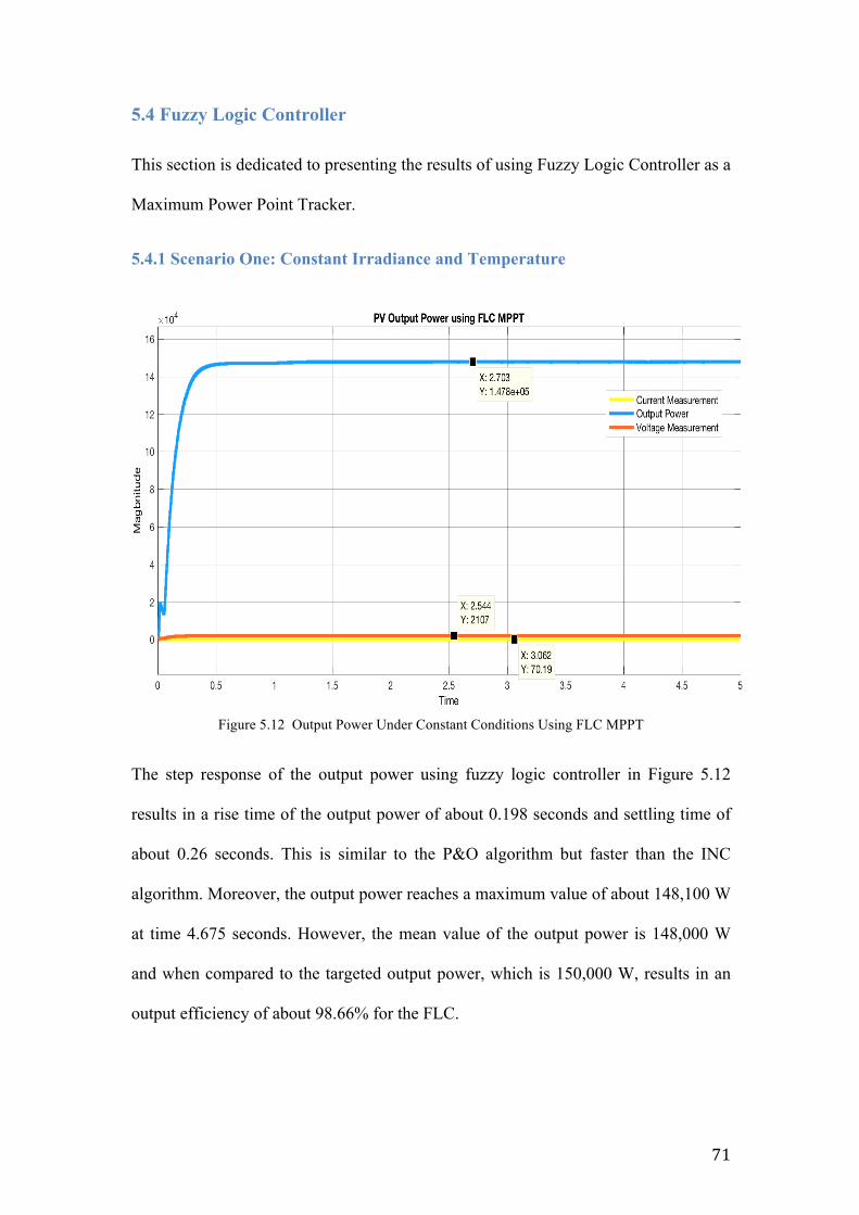
71
5.4 Fuzzy Logic Controller This section is dedicated to presenting the results of using Fuzzy Logic Controller as a
Maximum Power Point Tracker.
5.4.1 Scenario One: Constant Irradiance and Temperature
Figure 5.12 Output Power Under Constant Conditions Using FLC MPPT
The step response of the output power using fuzzy logic controller in Figure 5.12
results in a rise time of the output power of about 0.198 seconds and settling time of
about 0.26 seconds. This is similar to the P&O algorithm but faster than the INC
algorithm. Moreover, the output power reaches a maximum value of about 148,100 W
at time 4.675 seconds. However, the mean value of the output power is 148,000 W
and when compared to the targeted output power, which is 150,000 W, results in an
output efficiency of about 98.66% for the FLC.
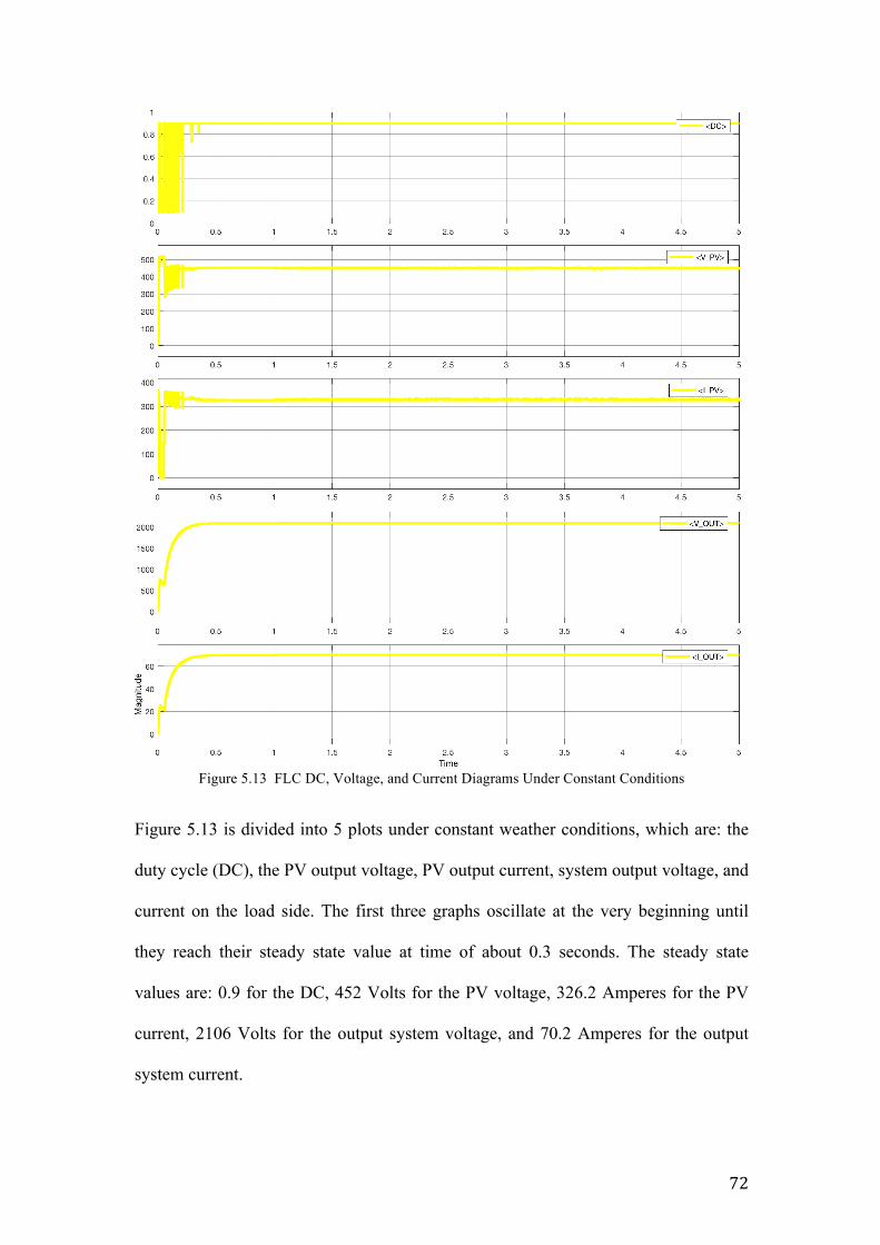
72
Figure 5.13 FLC DC, Voltage, and Current Diagrams Under Constant Conditions
Figure 5.13 is divided into 5 plots under constant weather conditions, which are: the
duty cycle (DC), the PV output voltage, PV output current, system output voltage, and
current on the load side. The first three graphs oscillate at the very beginning until
they reach their steady state value at time of about 0.3 seconds. The steady state
values are: 0.9 for the DC, 452 Volts for the PV voltage, 326.2 Amperes for the PV
current, 2106 Volts for the output system voltage, and 70.2 Amperes for the output
system current.
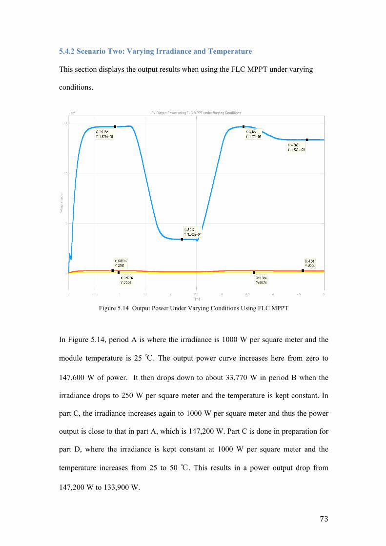
73
5.4.2 Scenario Two: Varying Irradiance and Temperature This section displays the output results when using the FLC MPPT under varying
conditions.
Figure 5.14 Output Power Under Varying Conditions Using FLC MPPT
In Figure 5.14, period A is where the irradiance is 1000 W per square meter and the
module temperature is 25 ℃. The output power curve increases here from zero to
147,600 W of power. It then drops down to about 33,770 W in period B when the
irradiance drops to 250 W per square meter and the temperature is kept constant. In
part C, the irradiance increases again to 1000 W per square meter and thus the power
output is close to that in part A, which is 147,200 W. Part C is done in preparation for
part D, where the irradiance is kept constant at 1000 W per square meter and the
temperature increases from 25 to 50 ℃. This results in a power output drop from
147,200 W to 133,900 W.
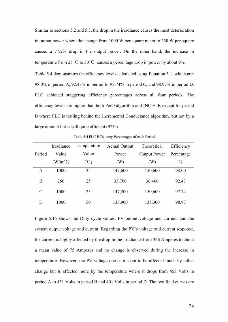
74
Similar to sections 5.2 and 5.3, the drop in the irradiance causes the most deterioration
in output power where the change from 1000 W per square meter to 250 W per square
caused a 77.2% drop in the output power. On the other hand, the increase in
temperature from 25 ℃ to 50 ℃ causes a percentage drop in power by about 9%.
Table 5.4 demonstrates the efficiency levels calculated using Equation 5.1, which are:
98.0% in period A, 92.43% in period B, 97.74% in period C, and 98.97% in period D.
FLC achieved staggering efficiency percentages across all four periods. The
efficiency levels are higher than both P&O algorithm and INC + IR except for period
B where FLC is trailing behind the Incremental Conductance algorithm, but not by a
large amount but is still quite efficient (92%)
Table 5.4FLC Efficiency Percentages of each Period
Period
Irradiance
Value
(W/m^2)
Temperature
Value
(℃)
Actual Output
Power
(W)
Theoretical
Output Power
(W)
Efficiency
Percentage
%
A 1000 25 147,600 150,600 98.00
B 250 25 33,700 36,460 92.43
C 1000 25 147,200 150,600 97.74
D 1000 50 133,900 135,300 98.97
Figure 5.15 shows the Duty cycle values, PV output voltage and current, and the
system output voltage and current. Regarding the PV’s voltage and current response,
the current is highly affected by the drop in the irradiance from 326 Amperes to about
a mean value of 75 Amperes and no change is observed during the increase in
temperature. However, the PV voltage does not seem to be affected much by either
change but is affected more by the temperature where it drops from 453 Volts in
period A to 451 Volts in period B and 401 Volts in period D. The two final curves are
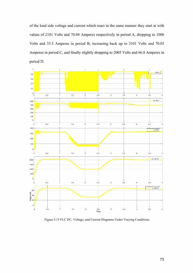
75
of the load side voltage and current which react in the same manner they start at with
values of 2101 Volts and 70.04 Amperes respectively in period A, dropping to 1006
Volts and 33.5 Amperes in period B, increasing back up to 2101 Volts and 70.03
Amperes in period C, and finally slightly dropping to 2005 Volts and 66.8 Amperes in
period D.
Figure 5.15 FLC DC, Voltage, and Current Diagrams Under Varying Conditions
76
Chapter 6 Conclusion
6.1 Research Objectives This research focused on the Maximum Power Point Tracking ability of a PV system
in order to determine the best possible method that can be used to generate the
optimum levels of power. This is intended to help decision-makers and solar energy
users understand how maximum power point tracking works, what factors affect it,
and how to enhance its efficiency.
The objectives of this research were: (1) to analyze multiple controllers in terms of
their Maximum Power Point Tracking ability when subjected to constant and varying
weather conditions (partial shading); and (2) study the effect of irradiance and
temperature change on the power output of a PV solar array. This was performed
through modeling and simulating three controllers, which are P&O, INC + IR, and
FLC, and comparing between them under two separate scenarios. The first scenario
was simulated under constant conditions of irradiance and temperature while the
second scenario was simulated under varying conditions of irradiance and
temperature. Since P&O and INC are reported to have similar efficiency percentages
as discussed in [39], this Thesis added an Integral Regulator to the INC in order to
evaluate the difference in efficiency between the P&O and INC + IR. This thesis
offers an analytical and methodological approach to realizing the qualitative
differences between the common MPPT techniques and how the enhancement of the
design will affect the output. It also aims at researching Artificial Intelligence
techniques such as Fuzzy Logic as they are projected to be the core of our technology
in the future. The following section reports on the findings of these two scenarios for
each controller.
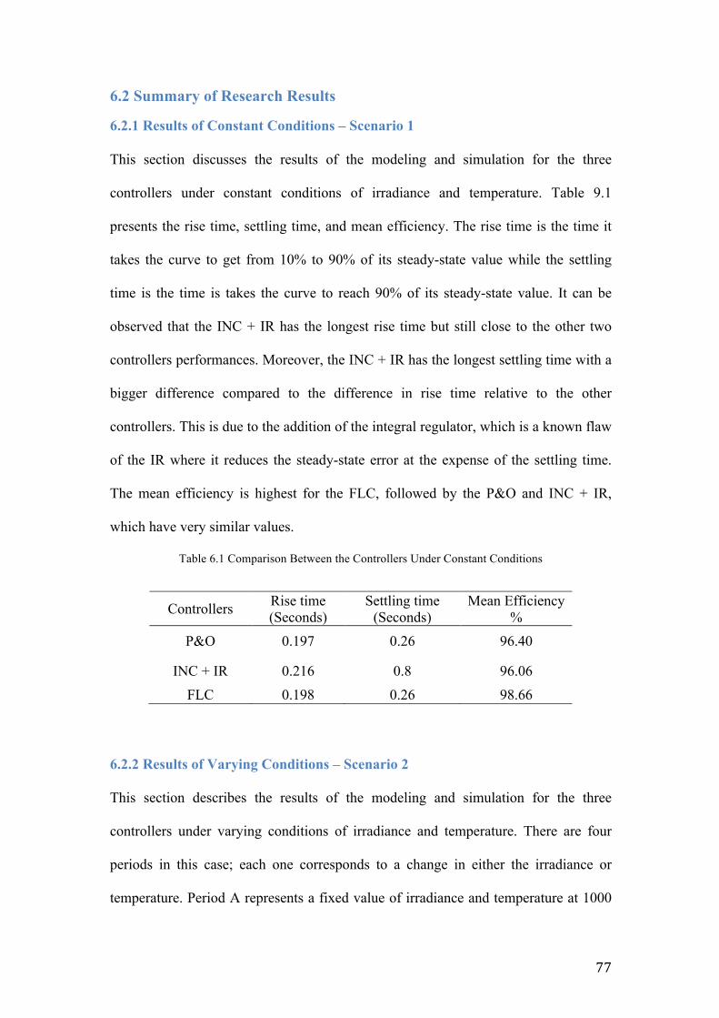
77
6.2 Summary of Research Results
6.2.1 Results of Constant Conditions – Scenario 1 This section discusses the results of the modeling and simulation for the three
controllers under constant conditions of irradiance and temperature. Table 9.1
presents the rise time, settling time, and mean efficiency. The rise time is the time it
takes the curve to get from 10% to 90% of its steady-state value while the settling
time is the time is takes the curve to reach 90% of its steady-state value. It can be
observed that the INC + IR has the longest rise time but still close to the other two
controllers performances. Moreover, the INC + IR has the longest settling time with a
bigger difference compared to the difference in rise time relative to the other
controllers. This is due to the addition of the integral regulator, which is a known flaw
of the IR where it reduces the steady-state error at the expense of the settling time.
The mean efficiency is highest for the FLC, followed by the P&O and INC + IR,
which have very similar values.
Table 6.1 Comparison Between the Controllers Under Constant Conditions
Controllers Rise time (Seconds)
Settling time (Seconds)
Mean Efficiency %
P&O 0.197 0.26 96.40
INC + IR 0.216 0.8 96.06 FLC 0.198 0.26 98.66
6.2.2 Results of Varying Conditions – Scenario 2 This section describes the results of the modeling and simulation for the three
controllers under varying conditions of irradiance and temperature. There are four
periods in this case; each one corresponds to a change in either the irradiance or
temperature. Period A represents a fixed value of irradiance and temperature at 1000
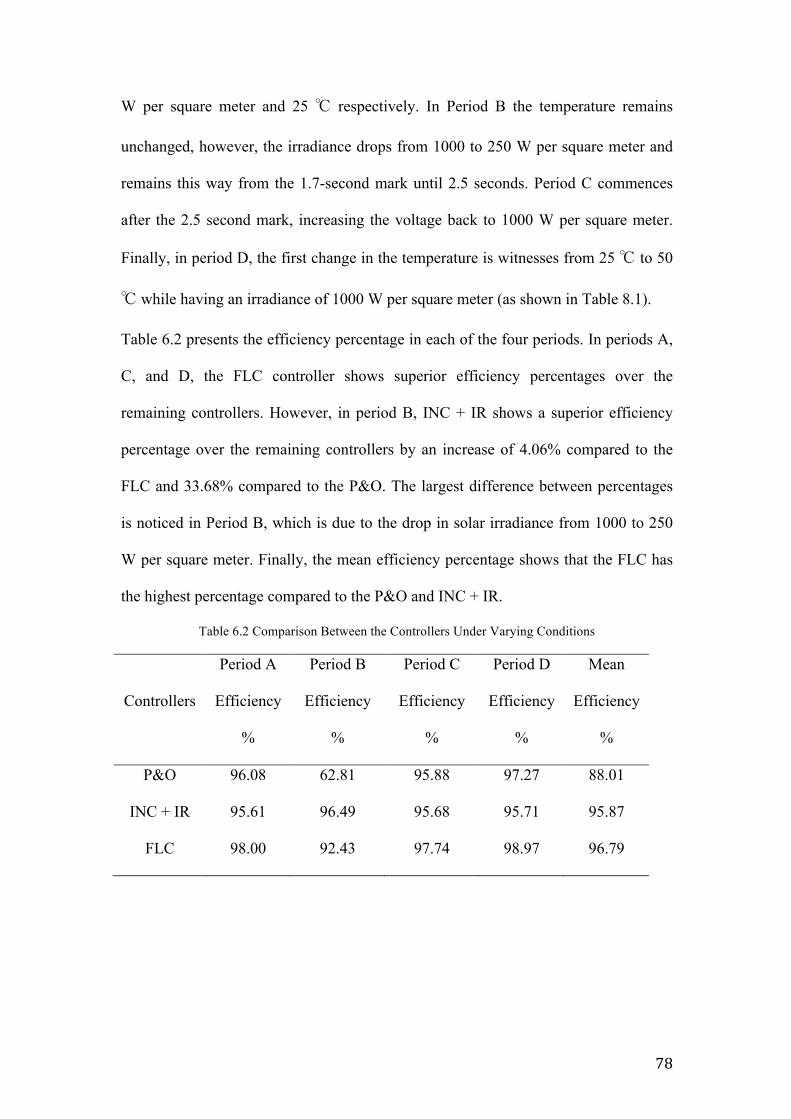
78
W per square meter and 25 ℃ respectively. In Period B the temperature remains
unchanged, however, the irradiance drops from 1000 to 250 W per square meter and
remains this way from the 1.7-second mark until 2.5 seconds. Period C commences
after the 2.5 second mark, increasing the voltage back to 1000 W per square meter.
Finally, in period D, the first change in the temperature is witnesses from 25 ℃ to 50
℃ while having an irradiance of 1000 W per square meter (as shown in Table 8.1).
Table 6.2 presents the efficiency percentage in each of the four periods. In periods A,
C, and D, the FLC controller shows superior efficiency percentages over the
remaining controllers. However, in period B, INC + IR shows a superior efficiency
percentage over the remaining controllers by an increase of 4.06% compared to the
FLC and 33.68% compared to the P&O. The largest difference between percentages
is noticed in Period B, which is due to the drop in solar irradiance from 1000 to 250
W per square meter. Finally, the mean efficiency percentage shows that the FLC has
the highest percentage compared to the P&O and INC + IR.
Table 6.2 Comparison Between the Controllers Under Varying Conditions
Controllers
Period A
Efficiency
%
Period B
Efficiency
%
Period C
Efficiency
%
Period D
Efficiency
%
Mean
Efficiency
%
P&O 96.08 62.81 95.88 97.27 88.01
INC + IR 95.61 96.49 95.68 95.71 95.87
FLC 98.00 92.43 97.74 98.97 96.79
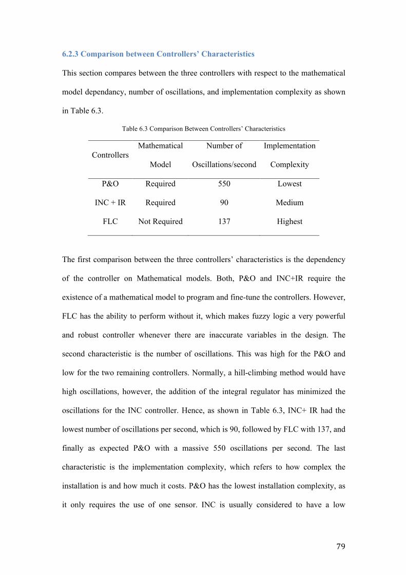
79
6.2.3 Comparison between Controllers’ Characteristics This section compares between the three controllers with respect to the mathematical
model dependancy, number of oscillations, and implementation complexity as shown
in Table 6.3.
Table 6.3 Comparison Between Controllers’ Characteristics
Controllers Mathematical
Model
Number of
Oscillations/second
Implementation
Complexity
P&O Required 550 Lowest
INC + IR Required 90 Medium
FLC Not Required 137 Highest
The first comparison between the three controllers’ characteristics is the dependency
of the controller on Mathematical models. Both, P&O and INC+IR require the
existence of a mathematical model to program and fine-tune the controllers. However,
FLC has the ability to perform without it, which makes fuzzy logic a very powerful
and robust controller whenever there are inaccurate variables in the design. The
second characteristic is the number of oscillations. This was high for the P&O and
low for the two remaining controllers. Normally, a hill-climbing method would have
high oscillations, however, the addition of the integral regulator has minimized the
oscillations for the INC controller. Hence, as shown in Table 6.3, INC+ IR had the
lowest number of oscillations per second, which is 90, followed by FLC with 137, and
finally as expected P&O with a massive 550 oscillations per second. The last
characteristic is the implementation complexity, which refers to how complex the
installation is and how much it costs. P&O has the lowest installation complexity, as
it only requires the use of one sensor. INC is usually considered to have a low
80
complexity but the addition of the integral regulator increases the system’s
complexity. FLC has the highest implementation complexity. In terms of cost, it is
difficult to get an accurate monetary value with the ever-decreasing prices of the
electronics; however, FLC generally has the highest cost [40].
6.3 Recommendations for Future Work Recommendations for future work include expanding the testing range of the
atmospheric temperature below 25 ℃ and above 50 ℃ as some parts of the world
reach these temperatures such as some countries in Europe and in the Middle East
respectively. Another point is to study the effect of changing both the temperature and
irradiance at the same time as that may occur in some instances and study its effect on
the output power. Moreover, another recommendation is to enhance and compare the
results of both the P&O algorithm and FLC by adding an integral regulator to P&O
and adding PID controller to FLC and making it an adaptive FLC. Another,
recommendation is to increase the number of rules used in FLC and study the effect
on output efficiency. A final further work recommendation is to connect the PV
standalone system to the grid and make the necessary adjustments to the system, so
that a more comprehensive result of the actual generated electricity can be reached.
81
References:
[1] U.S Department of Energy, Smart Grid: an introduction. [Online]. Available: https://energy.gov/oe/downloads/smart-grid-introduction
[2] “What is the Smart Grid?” SmartGrid.gov. [Online]. Available: https://www.smartgrid.gov/the_smart_grid/smart_grid.html. [Accessed: 20-Feb-2018].
[3] Nema, “Smart Grid: What is it and why is it important?,” NEMA - Setting Standards for Excellence. [Online]. Available: https://www.nema.org/Policy/Energy/Smartgrid/Pages/default.aspx. [Accessed: 20-Feb-2018].
[4] DEWA, Powering Dubai on a smart, renewable grid, Smartdubai.ae, May 2014. [Online]. Available: http://www.smartdubai.ae/partner_story_two.php. [Accessed: 23- Feb- 2018].
[5] WiMax Forum, System Profile Requirements for Smart Grid Applications, February 05,2013. Available: http://files.wimaxforum.org/Document/Download/WMF-T31-002R010v01 Wimax_System_Profile_Requirements_for_SmartGrid_Applications
[6] “Power Systems Simulation Laboratory,” A comparison between conventional grid and the Smart Grid | Power Systems Simulation Laboratory. [Online]. Available: http://www.itee.uq.edu.au/pssl/drupal7_with_innTheme/?q=node%2F347. [Accessed: 20-Feb-2018].
[7] C. P. Vineetha and C. A. Babu, “Smart grid challenges, issues and solutions,” 2014 International Conference on Intelligent Green Building and Smart Grid (IGBSG), 2014.
[8] "Photovoltaic Solar Electric", SEIA. [Online]. Available: https://www.seia.org/initiatives/photovoltaic-solar-electric. [Accessed: 12- Mar- 2018].
[9] "Solar Photovoltaic System Design Basics", Energy.gov, 2013. [Online]. Available: https://energy.gov/eere/solar/articles/solar-photovoltaic-system-design-basics. [Accessed: 12- Mar- 2018].
[10] Energy Informative, 2013. [11] Solarvis Energy , "Advantages and disadvantages of Solar Photovoltaic | Solar
Energy News", Solarvis.energy. [Online]. Available: https://www.solarvis.energy/advantages-and-disadvantages-of-solar-photovoltaic/. [Accessed: 12- Mar- 2018].
[12] S. Sundaram, K. Sheeba and J. Babu, "Grid Connected Photovoltaic Systems: Challenges and Control Solutions - A Potential Review", International Journal of Electronics and Electrical Engineering, pp. 463-473, 2016.
[13] E. Camacho, T. Samad, M. Sanz and I. Hiskens, Control for Renewable Energy and Smart Grids. IEEE.
[14] J. Wippler, "» MPPT hunting » JeeLabs", Jeelabs.org, 2013. [Online]. Available: https://jeelabs.org/2013/05/21/mppt-hunting/. [Accessed: 09- Jan- 2019
[15] D. Bromberg, "Install tip: Know how inverter MPPT functionality affects performance", Solar Power World, 2018. [Online]. Available: https://www.solarpowerworldonline.com/2018/03/install-tip-inverter-mppt-functionality-affects-performance/. [Accessed: 09- Jan- 2019]
[16] Nader Anani, M. Shahid, Omar Al-kharji, Joao Ponciano, “A CAD Package for Modeling and Simulation of PV Arrays under Partial Shading Conditions,” Energy Procedia, Volume 42, 2013, Pages 397-405, ISSN 1876-6102,
82
https://doi.org/10.1016/j.egypro.2013.11.040. Available at: http://www.sciencedirect.com/science/article/pii/S1876610213017426
[17] G. Patel, D. Patel and K. Paghdal, "ANALYSIS OF P&O MPPT ALGORITHM FOR PV SYSTEM", International Journal of Electrical and Electronics Engineering (IJEEE), vol. 5, no. 6, pp. 1-10, 2016. Available: http://oaji.net/articles/2016/1879-1481110428.pdf. [Accessed 14 January 2019].
[18] A. Atallah, A. Abdelaziz and R. Jumaah, "IMPLEMENTATION OF PERTURB AND OBSERVE MPPT OF PV SYSTEM WITH DIRECT CONTROL METHOD USING BUCK AND BUCKBOOST CONVERTERS", Emerging Trends in Electrical, Electronics & Instrumentation Engineering, vol. 1, no. 1, 2014. Available: https://airccse.com/eeiej/papers/1114eeiej03.pdf. [Accessed 14 January 2019].
[19] C. Panchano, "PERTURB AND OBSERVE ALGORITHMS FOR DC LOAD SYSTEMS", Master's, Newcastle University, 2014.
[20] U. Patel, D. Sahu and D. Tirkey, "Maximum Power Point Tracking Using Perturb & Observe Algorithm and Compare With another Algorithm", International Journal of Digital Application & Contemporary research, vol. 2, no. 2, 2013. Available: http://ijdacr.com/uploads/papers/DhaneshwariSahu_paper.pdf. [Accessed 14 January 2019].
[21] R. Mayfield, "The Highs and Lows of Photovoltaic System Calculations", Electrical Construction & Maintenance (EC&M) Magazine, 2012. [Online]. Available: https://www.ecmweb.com/green-building/highs-and-lows-photovoltaic-system-calculations. [Accessed: 14- Jan- 2019].
[22] M. Chaaban, "Temperature and PV Performance Optimization | AE 868: Commercial Solar Electric Systems", E-education.psu.edu. [Online]. Available: https://www.e-education.psu.edu/ae868/node/878. [Accessed: 14- Jan- 2019].
[23] M. R. H. Bipu, S. M. S. M. Chowdhury, M. Dautta, M. Z. Nain and S. I. Khan, "Modeling and analysis of maximum power point tracking algorithms using MATLAB/Simulink," 2015 International Conference on Electrical Engineering and Information Communication Technology (ICEEICT), Dhaka, 2015, pp. 1-6. doi: 10.1109/ICEEICT.2015.7307412
[24] M. Abulkadir, A. Samosir, A. Yatim and S. Yusuf, A NEW APPROACH OF MODELLING, SIMULATION OF MPPT FOR PHOTOVOLTAIC SYSTEM IN SIMULINK MODEL, 8th ed. ARPN Journal of Engineering and Applied Sciences, 2013, p. 491.
[25] G. Siegfried, "Many-Valued Logic", The Stanford Encyclopedia of Philosophy (Winter 2017 Edition), Edward N. Zalta (ed.), Available: https://plato.stanford.edu/archives/win2017/entries/logic-manyvalued/.
[26] D. Dubois, F. Esteva, L. Godo and H. Prade, FUZZY-SET BASED LOGICS — AN HISTORY-ORIENTED PRESENTATION OF THEIR MAIN DEVELOPMENTS, 8th ed. Elsevier BV, 2007.
[27] B. Ankayarkanni and L. Ezel, "GABC based neuro-fuzzy classifier with multi kernel segmentation for satellite image classification", Biomedical Research, vol. 29, no. 21, 2016. Available: http://www.alliedacademies.org/articles/gabc-based-neurofuzzy-classifier-with-multi-kernel-segmentation-for-satellite-image-classification.html. [Accessed 14 January 2019].
[28] K. Thórisson and H. Vilhjálmsson, "Intro to AI: Fuzzy Logic", Ru.is, 2007. [Online]. Available: http://www.ru.is/faculty/thorisson/courses/v2007/gervigreind/FuzzyLogic.html. [Accessed: 14- Jan- 2019].
[29] B. Singh and A. Mishra, "Fuzzy Logic Control System and its Applications", IRJET, vol. 2, no. 8, 2015. [Accessed 14 January 2019].
83
[30] J. Paulusová, "Fuzzy logic autotuning methods for predictive controller", Posterus.sk, 2010. [Online]. Available: http://www.posterus.sk/?p=7961. [Accessed: 14- Jan- 2019].
[31] R. Vicerra et al., "A multiple level MIMO fuzzy logic based intelligence for multiple agent cooperative robot system", TENCON 2015 - 2015 IEEE Region 10 Conference, 2015. Available: 10.1109/tencon.2015.7372985 [Accessed 14 January 2019].
[32] C. Lee, Fuzzy Logic in Control Systems: Fuzzy Logic Controller-Part I, 20th ed. IEEE, 1990, pp. 404 -415.
[33] N. Hussein Selman, "Comparison Between Perturb & Observe, Incremental Conductance and Fuzzy Logic MPPT Techniques at Different Weather Conditions", International Journal of Innovative Research in Science, Engineering and Technology, vol. 5, no. 7, pp. 12556-12569, 2016. Available: 10.15680/ijirset.2016.0507069 [Accessed 10 January 2019].
[34] N. de Reus, Assessment of benefits and drawbacks of' using fuzzy logic especially in fire control systems, 35th ed. TNO, 1994.
[35] M. Quamruzzaman, , Nur, Matin, Mahmud, Alam, “Highly efficient maximum power point tracking using DC–DC coupled inductor single-ended primary inductance converter for photovoltaic power systems.” International Journal of Sustainable Energy. Vol.35. pp.1-19, 2014. DOI: 10.1080/14786451.2014.961922.
[36] "Detailed Model of a 100-kW Grid-Connected PV Array- MATLAB & Simulink", Mathworks.com, [Online]. Available: https://www.mathworks.com/help/physmod/sps/examples/detailed-model-of-a-100-kw-grid-connected-pv-array.html. [Accessed: 21- Jan- 2019].
[37] A. Pradhan and B. Panda, "A Simplified Design and Modeling of Boost Converter for Photovoltaic Sytem", International Journal of Electrical and Computer Engineering (IJECE), vol. 8, no. 1, p. 141, 2018. Available: 10.11591/ijece.v8i1.pp141-149 [Accessed 21 January 2019].
[38] R. Erickson and D. Maksimović, Fundamentals of power electronics, 2nd ed. New York: Kluwer Academic, 2004.
[39] D. Sera, L. Mathe, T. Kerekes, S. Spataru and R. Teodorescu, "On the Perturb-and-Observe and Incremental Conductance MPPT Methods for PV Systems", IEEE Journal of Photovoltaics, vol. 3, no. 3, pp. 1070-1078, 2013. Available: 10.1109/jphotov.2013.2261118 [Accessed 21 January 2019].
[40] A. Reza Reisi, M. Hassan Moradi and S. Jamasb, "Classification and comparison of maximum power point tracking techniques for photovoltaic system: A review", Renewable and Sustainable Energy Reviews, vol. 19, pp. 433-443, 2013. Available: 10.1016/j.rser.2012.11.052.
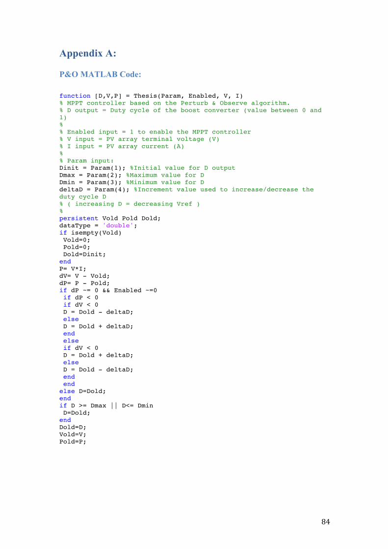
84
Appendix A:
P&O MATLAB Code: function [D,V,P] = Thesis(Param, Enabled, V, I) % MPPT controller based on the Perturb & Observe algorithm. % D output = Duty cycle of the boost converter (value between 0 and 1) % % Enabled input = 1 to enable the MPPT controller % V input = PV array terminal voltage (V) % I input = PV array current (A) % % Param input: Dinit = Param(1); %Initial value for D output Dmax = Param(2); %Maximum value for D Dmin = Param(3); %Minimum value for D deltaD = Param(4); %Increment value used to increase/decrease the duty cycle D % ( increasing D = decreasing Vref ) % persistent Vold Pold Dold; dataType = 'double'; if isempty(Vold) Vold=0; Pold=0; Dold=Dinit; end P= V*I; dV= V - Vold; dP= P - Pold; if dP ~= 0 && Enabled ~=0 if dP < 0 if dV < 0 D = Dold - deltaD; else D = Dold + deltaD; end else if dV < 0 D = Dold + deltaD; else D = Dold - deltaD; end end else D=Dold; end if D >= Dmax || D<= Dmin D=Dold; end Dold=D; Vold=V; Pold=P;