ENGSTRUCT-D-15-00999.pdf

7/23/2019 ENGSTRUCT-D-15-00999.pdf

http://slidepdf.com/reader/full/engstruct-d-15-00999pdf 1/36

Engineering Structures

Manuscript Draft

Manuscript Number: ENGSTRUCT-D-15-00999

Title: Using data mining algorithms to predict the bond strength of FRP NSM systems in concrete

Article Type: Research Paper

Keywords: FRP; NSM; Bond; Guidelines; Data Mining

Abstract: This paper presents the effectiveness of soft computing algorithms in analyzing the bond

behavior of fiber reinforced polymer (FRP) systems inserted in the cover of concrete elements,

commonly known as the near-surface mounted (NSM) technique. It focuses on the use of Data Mining

(DM) algorithms as an alternative to the existing guidelines' models to predict the bond strength of

FRP NSM systems. To ease and spread the use of DM algorithms, a web-based tool is presented. This

tool was developed to allow an easy use of the DM prediction models presented in this work, where the

user simply provides the values of the input variables, the same as those used by the guidelines, in

order to get the predictions. The results presented herein show that the DM based models are robustand more accurate than the guidelines' models and can be considered as a relevant alternative to those

analytical methods.

7/23/2019 ENGSTRUCT-D-15-00999.pdf


Formulations for predicting the bond strength in FRP NSM systems are analyzed

The prediction’s accuracy of ACI 4402R-08 and HB 305 –2008 guidelines are tested

Alternative formulations based on data mining algorithms are suggested

The results showed that the data mining algorithms can be a good alternative

A website is presented to ease the use of the data mining models developed

ghlights (for review)

ck here to download Highlights (for review): Highlights.docx

http://ees.elsevier.com/engstruct/download.aspx?id=623124&guid=f93e03a4-7551-4f2c-91c5-b4a80a96d9eb&scheme=1

http://ees.elsevier.com/engstruct/download.aspx?id=623124&guid=f93e03a4-7551-4f2c-91c5-b4a80a96d9eb&scheme=1

7/23/2019 ENGSTRUCT-D-15-00999.pdf



behavior of fiber reinforced polymer (FRP) systems inserted in the cover of concrete elements, commonly

known as the near-surface mounted (NSM) technique. It focuses on the use of Data Mining (DM)

algorithms as an alternative to the existing guidelines’ models to predict the bond strength of FRP NSM

systems. To ease and spread the use of DM algorithms, a web-based tool is presented. This tool was

developed to allow an easy use of the DM prediction models presented in this work, where the user

simply provides the values of the input variables, the same as those used by the guidelines, in order to get

the predictions. The results presented herein show that the DM based models are robust and more

accurate than the guidelines’ models and can be considered as a relevant alternative to those analytical

methods.

bstract

ck here to download Abstract: Abstract.docx

http://ees.elsevier.com/engstruct/download.aspx?id=623125&guid=2dd5b14b-524d-4d76-8220-1871c53356a4&scheme=1

http://ees.elsevier.com/engstruct/download.aspx?id=623125&guid=2dd5b14b-524d-4d76-8220-1871c53356a4&scheme=1

7/23/2019 ENGSTRUCT-D-15-00999.pdf


USING DATA MINING ALGORITHMS TO PREDICT THE BOND STRENGTH OF FRP NSM

SYSTEMS IN CONCRETE

Mário R. F. Coelho1,2

, José M. Sena-Cruz1,3

, Luís A. C. Neves4,5

, Marta Pereira6,7

,

Paulo Cortez

8,9

, Tiago Miranda

1,10

1 ISISE, University of Minho, Department of Civil Engineering, Campus de Azurém, 4810-058

Guimarães, Portugal

2E-mail: [email protected]

3 E-mail: [email protected]; Corresponding author

4 University of Nottingham, Department of Civil Engineering, Nottingham, United Kingdom

5 E-mail: [email protected]

6 University of Minho, Department of Information Systems, Campus de Azurém, 4810-058 Guimarães,

Portugal

7 E-mail: [email protected]

8 ALGORITMI Centre, University of Minho, Department of Information Systems, Campus de Azurém,

4810-058 Guimarães, Portugal

9E-mail: [email protected]

10

E-mail: [email protected]


behavior of fiber reinforced polymer (FRP) systems inserted in the cover of concrete elements, commonly

known as the near-surface mounted (NSM) technique. It focuses on the use of Data Mining (DM)

algorithms as an alternative to the existing guidelines’ models to predict the bond strength of FRP NSM

systems. To ease and spread the use of DM algorithms, a web-based tool is presented. This tool was

developed to allow an easy use of the DM prediction models presented in this work, where the user

simply provides the values of the input variables, the same as those used by the guidelines, in order to get

the predictions. The results presented herein show that the DM based models are robust and more

accurate than the guidelines’ models and can be considered as a relevant alternative to those analytical

methods.

Keywords: FRP; NSM; Bond; Guidelines; Data Mining

anuscript

ck here to download Manuscript: Manuscript.docx Click here to view linked References

mailto:[email protected]















http://ees.elsevier.com/engstruct/download.aspx?id=623126&guid=043758ee-23bb-47f0-9595-ffbfb0bd5a71&scheme=1

http://ees.elsevier.com/engstruct/viewRCResults.aspx?pdf=1&docID=15806&rev=0&fileID=623126&msid=97D806D0-F9AA-4CCD-B3B8-FBC26EA372B8

http://ees.elsevier.com/engstruct/viewRCResults.aspx?pdf=1&docID=15806&rev=0&fileID=623126&msid=97D806D0-F9AA-4CCD-B3B8-FBC26EA372B8

http://ees.elsevier.com/engstruct/download.aspx?id=623126&guid=043758ee-23bb-47f0-9595-ffbfb0bd5a71&scheme=1






7/23/2019 ENGSTRUCT-D-15-00999.pdf


1. Introduction

The strengthening technique that uses fiber reinforced polymers (FRP) inserted in the concrete cover of

the element to be strengthened is known as near-surface mounted (NSM) technique. In the last 15 years

intensive research has been devoted to the NSM technique, becoming a widespread technique in practical

applications in the last years [1, 2].

Nevertheless, the NSM technique presents many challenges to overcome. In particular, the

characterization of the transfer of stresses between the FRP system and the surrounding concrete, i.e. the

bond behavior of FRP NSM systems, is not yet completely understood. The bond behavior has been

studied through direct pullout tests (DPT) and/or beam pullout tests (BPT). Figure 1 presents a generic

example of both tests including some of the parameters used to quantify the bond strength discussed later

in this paper.

In Coelho et al. [2], a review on these bond tests was presented and two databases collecting a

wide range of DPT and BPT results were presented and used for better understand key parameters

affecting the bond performance of the NSM system. These databases were also used to evaluate the

accuracy and limitations of two of the most relevant guidelines for predicting the bond strength of FRP

NSM systems in concrete. The first formulation is included in the “Guide for the Design and Construction

of Externally Bonded FRP Systems for Strengthening Concrete Structures” from the American Concrete

Institute [3]. The second guideline is the “Design handbook for reinforced concrete structures retrofitted

with FRP and metal plates: beams and slabs” from Standards Australia [4]. In this paper, those guidelines

will be referred to as ACI and SA, respectively.

The difficulties in modeling the bond performance arise from the high complexity of the NSM

technique which involves three different materials (FRP, adhesive and concrete) and two different

interfaces (FRP/adhesive and adhesive/concrete). The variety of properties (physical and mechanical) of

each material and interface leads to the existence of several failure modes. However, ACI and SA

guidelines are not able to capture explicitly all of them. On the other hand, that large variety of properties

is associated to a large number of variables and their influence on the bond behavior of FRP NSM is far

from being completely understood [2].

In an attempt to provide an alternative to the referred guidelines, this paper introduces the use of

prediction models based on Data Mining (DM) algorithms. In order to provide some insights on the use of

DM in structural engineering, the following section presents a brief overview on DM, focusing on its use

7/23/2019 ENGSTRUCT-D-15-00999.pdf


7/23/2019 ENGSTRUCT-D-15-00999.pdf


input and output variables, in what is often termed as “black - box” models [6]. As an advantage, the DM

approach simplifies the data analysis process [7]. In effect, DM models tend to be more flexible, being

capable of predicting complex nonlinear mappings and dealing with large amounts of data or noise. Such

model learning flexibility often leads to higher predictive performances when compared with classical

statistical models (e.g., multiple regression).

DM algorithms have been successfully used in regression tasks in many areas, including Civil

Engineering [8-11]. More specifically, in the field of concrete structures strengthened with FRP systems

there are examples where DM algorithms have been used to predict the lateral confinement coefficient for

reinforced concrete columns wrapped with CFRP [12], the strength of FRP confined concrete cylinders

[13] or the shear strength of reinforced concrete beams reinforced with FRP systems [14] . According to

the author’s best knowledge, only one work of their authorship is available where DM algorithms were

applied to predict the bond strength of FRP NSM systems in concrete [15].

In this work, two DM algorithms were used: the Artificial Neural Networks (ANN) and the

Support Vector Machines (SVM). These DM algorithms are briefly presented in the following sections.

2.1. Artificial Neural Networks

The Artificial Neural Network (ANN) is an algorithm that is inspired in the behavior of the human central

nervous system. Hence, the learning ANN algorithm aims at finding the best connection weights in which

a set of artificial neurons should communicate with each other in order to attain a certain target [16].

Figure 2 presents two ANN examples: (i) Figure 2(a) corresponds to a multiple linear regression,

which is a widely known and commonly accepted type of regression model. This is an example of the

simplest ANN, without hidden nodes; (ii) Figure 2( b) corresponds to a more complex ANN with one

hidden layer and two hidden neurons (HN). As it can be seen, the only difference between them is the

existence or not of an intermediate layer of hidden neurons.

In the multiple linear regression, several input variables ( x) affected by different weights are

combined and an output variable ( y) is obtained. In the ANN with one hidden layer intermediary weights

are also introduced thus a nonlinear relation between x and y can be obtained. The number of hidden

layers and neurons can be different from this example and, by increasing them, the degree of nonlinearity

increases.

7/23/2019 ENGSTRUCT-D-15-00999.pdf


If the value of y is known a priori, then the multiple linear regression model is an expression

identic to expression (1), where the only unknown is the set of weights (w) that make the equality true. In

the case of ANN with hidden layers, such an expression is no longer straightforward to obtain. However,

a similar procedure minimizing the difference between the predicted and observed values can be used to

find the optimal weights, in a process called training.

The type of ANN adopted in this work uses only one hidden layer since this is the simplest

nonlinear ANN and was found to attain good results. The number of hidden neurons determined during

the analysis by comparing the quality of fit with increasing number of neurons (between 0 and 9) and

selecting the one which presents lower prediction errors (when considering training data).

0 1

n

i ii

y w w x

(1)

2.2. Support Vector Machines

Support vector machines (SVM) can be seen as an upgrade to the ANN and were initially developed for

classification tasks [17]. Considering the classification purpose, the basic concept of SVM is finding an

optimal hyperplane for linearly separate patterns, i.e., finding the plane which maximizes the separation

between the different patterns that exist in the analyzed data. To ease the understanding of SVM

functioning in a classification task, Figure 3 presents an example of a database with two input variables

( x1 and x2) divided in two patterns (circles and squares). In the database real space (middle chart in Figure

3) those patterns can only be separated using a curved line. However, it can be found a function which,

applied to the original data, can transform it into a new high dimensional space where the two patterns

can actually be separated by a straight line. SVM algorithm optimizes the position of that single line such

that it maximizes the separation of the two patterns. Several division lines can exist and are represented as

full lines in the left side of Figure 3. However, in this case, the line that maximizes the separation of the

patterns is the thicker one represented in that figure. Remark that, in more complex examples (with

several variables), the lines would be actually hyperplanes, as referred before. In the end, since the

optimal hyperplane is known, the relative position of all the data points, especially those passed by the

dashed lines (designated by support vectors) is also known. Hence, a model traducing the separation of

the patterns can be defined which corresponds to the classification model that was sought in the

beginning.

7/23/2019 ENGSTRUCT-D-15-00999.pdf


SVM were latter extended to also perform regression tasks, which are the important ones in the

scope of this work, being its functioning similar to the classification case. However, in regression, another

function will transform the original data in order to find a line that passes through all data points (right

chart in Figure 3). That line is the regression function which allows predict the value of each data point.

Since finding such a line is quite complex, there are two new important parameters in the SVM for

regression, namely the regularization parameter (C ) and a loss function that in this work is the -

insensitive ( ). The first defines the tradeoff between complexity and accuracy of the model to be found,

while the second defines the width of a region in which the data points inside it are assumed to be on the

regression line, thus an insensitive region. The data points outside this region are the support vectors in

the regression SVM.

Besides these two parameters, the success of SVM for regression tasks is influenced by a kernel

function. In this work, the Gaussian radial basis kernel function was adopted (2). This has only one

hyperparameter, , which was adjusted using a greedy search (between 2-15

and 23). Similar procedure

was also adopted for parameter , while parameter C was considered equal to 3 [18].

2

, ' ' , 0k x x exp x x (2)

2.3. Rminer tool

Nowadays, there are several tools that allow an easy application of DM algorithms with a limited

knowledge of the mathematical background required for implementation. In this work, the rminer library

[18] of the R Statistical Environment [19] was adopted, since it is particularly suited for generating ANN

and SVM data-driven models.

Among the several features included in rminer, in this work the functions mining , fit and predict

were used. For simplicity, the functions will be described using a parallel with a simple regression model.

The function fit allows finding an analytical expression in the form y = mx + b with m and b

adjusted to the database in analysis. Having the expression calibrated, predict gives the results ( y) for new

values of the independent variable ( x) by replacing it in the expression found by fit . The function mining

is a more sophisticated function. It performs several runs (i.e., sequences of fit and predict executions)

under a user selected validation method. It is important to emphasize that, while fit uses the entire

database to adjust a model, mining only uses part of it, being the fitted model tested in unseen data (i.e.,

test set). This aspect is very important since it allows evaluating the performance of the adjusted model

7/23/2019 ENGSTRUCT-D-15-00999.pdf


when applied to new data (depending on the validation method), thus measuring the true generalization

capacity of the DM model. In this work, a holdout split validation method was adopted, in which 2/3 of

the data entries were randomly selected as training data and the remaining 1/3 samples were used as test

data. Another important difference is that only fit function allows storing a model that can be then used,

like an analytical expression, to perform new predictions. In fact, depending on the chosen division of sets

and number of runs, for example, mining function can produce a huge number of models. For practical

reasons, the rminer library does not store any of these models.

3. Tests and analyses

The following paragraphs present the databases of tests used in this work. Then the ACI and SA

analytical formulations, used as reference, are presented. Finally, the DM analyses carried out in this

work are detailed.

3.1. Databases of pullout tests

As referred, two databases of pullout tests were built, one including 363 direct pullout tests (DPT) and

other with 68 beam pullout tests (BPT). In the context of the present work, it was decided to build up a

webpage to store the referred databases (www.frpbondata.civil.uminho.pt). It is believed that providing

the scientific community free access to the vast majority of pullout tests available in the literature makes

the process of continuously improving the existing prediction models faster and easier. It is expected that,

with the contribution of all the researchers working in this field, this website will be continuously

updated.

The referred website includes, besides the databases, a page to perform predictions of the

maximum pullout force ( F fmax) using different formulations. It includes ACI and SA guidelines and the

DM models developed herein. It is also believed that, by providing in the website an easy way of using

and testing DM models, the acceptance and use of such powerful tools will increase. Hence, providing the

required input variables, results obtained using all the prediction formulations described herein will be

readily available.

To help the community in improving prediction models for NSM bond behavior a detailed and

comprehensive data visualization tool is also included in the webpage. In addition, a Forum is also

available to ease the interaction between all the researchers contributing for the website.

http://www.frpbondata.civil.uminho.pt/




7/23/2019 ENGSTRUCT-D-15-00999.pdf


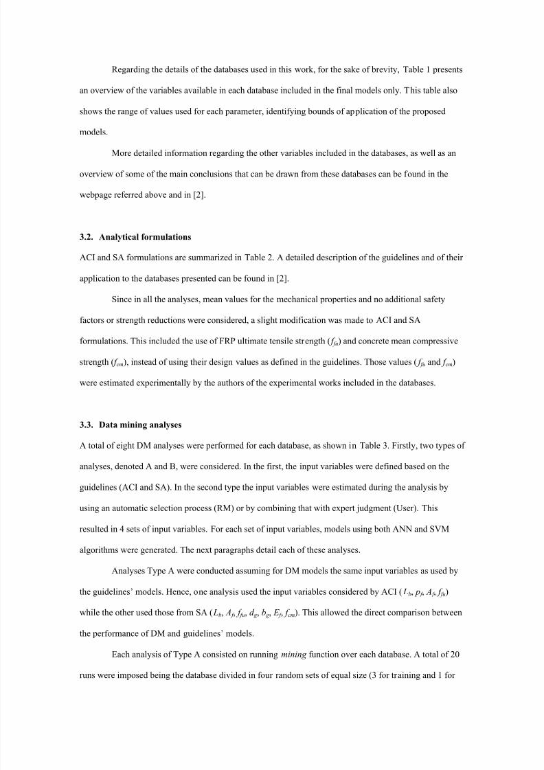
Regarding the details of the databases used in this work, for the sake of brevity, Table 1 presents

an overview of the variables available in each database included in the final models only. This table also

shows the range of values used for each parameter, identifying bounds of application of the proposed

models.

More detailed information regarding the other variables included in the databases, as well as an

overview of some of the main conclusions that can be drawn from these databases can be found in the

webpage referred above and in [2].

3.2. Analytical formulations

ACI and SA formulations are summarized in Table 2. A detailed description of the guidelines and of their

application to the databases presented can be found in [2].

Since in all the analyses, mean values for the mechanical properties and no additional safety

factors or strength reductions were considered, a slight modification was made to ACI and SA

formulations. This included the use of FRP ultimate tensile strength ( f fu) and concrete mean compressive

strength ( f cm), instead of using their design values as defined in the guidelines. Those values ( f fu and f cm)

were estimated experimentally by the authors of the experimental works included in the databases.

3.3. Data mining analyses

A total of eight DM analyses were performed for each database, as shown in Table 3. Firstly, two types of

analyses, denoted A and B, were considered. In the first, the input variables were defined based on the

guidelines (ACI and SA). In the second type the input variables were estimated during the analysis by

using an automatic selection process (RM) or by combining that with expert judgment (User). This

resulted in 4 sets of input variables. For each set of input variables, models using both ANN and SVM

algorithms were generated. The next paragraphs detail each of these analyses.

Analyses Type A were conducted assuming for DM models the same input variables as used by

the guidelines’ models. Hence, one analysis used the input variables considered by ACI ( Lb, p f , A f , f fu)

while the other used those from SA ( Lb, A f , f fu, d g , b g , E f , f cm). This allowed the direct comparison between

the performance of DM and guidelines’ models.

Each analysis of Type A consisted on running mining function over each database. A total of 20

runs were imposed being the database divided in four random sets of equal size (3 for training and 1 for

7/23/2019 ENGSTRUCT-D-15-00999.pdf


testing). Then the prediction error metrics fluctuation was analyzed in order to check generalization

capacity of each DM algorithm. To this purpose, the 95% t-student confidence interval was adopted.

Finally, the error metrics obtained in all the 20 runs were averaged to allow comparisons between model’s

accuracy.

In analyses Type B, it was assumed that the input variables were not known a priori. Hence,

besides the four and seven variables used by ACI and SA, respectively, all the numeric variables present

in more than 2/3 of the records in each database were also included. This resulted in more than 20 input

variables available on each database at the beginning of the calibration process.

The same procedure used in the analyses Type A was used for these new and larger databases. In

the end of the mining sequence, a sensitivity analysis was performed in order to identify the most

important variables in a backward selection procedure. After identifying the most important variables, the

procedure was repeated with the limited input variables. This process was carried out several times, being

the number of input variables successively reduced. In the end, a final set of input variables could be

proposed as well as the DM models using those input variables.

Since this sensitivity analysis is influenced by the representativeness of each variable in the

database, in some cases the final set of variables was found to be meaningless for design purposes. Hence,

a different type of models were generated, taking into account the evolution of the variable’s importance

in the sensitivity analyses and also including all the variables thought meaningful for design.

Since in the first case the variables were chosen taking into account only the rminer sensitivity

analysis, these were designated by RM. In the second case, since the choice was made by the user, the

designation User was adopted instead.

Finally, it should be emphasized that all the analyses carried out used the maximum pullout force

( F fmax) as the only output variable. Also, in all the analyses, variables normalization was considered using

a zero mean and a one standard deviation transformation for all input and output variables (-1 to 1 scale).

Then, the inverse procedure was performed for the output variable in order to export it in its original

scale.

4. Results

For each analysis three error metrics were calculated, namely, the mean absolute error ( MAE ), the root

mean squared error ( RMSE ) and squared correlation coefficient ( R2). Those are defined in the equations

7/23/2019 ENGSTRUCT-D-15-00999.pdf


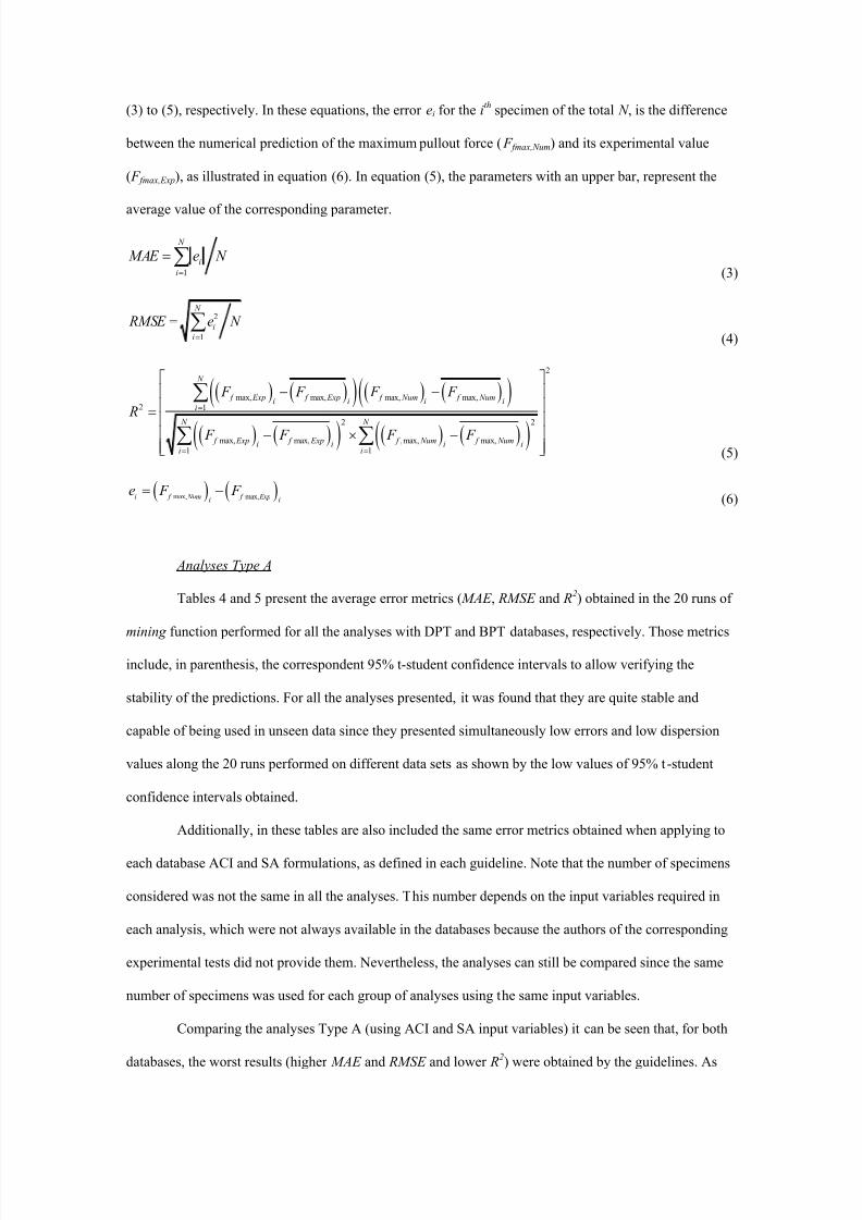
(3) to (5), respectively. In these equations, the error ei for the ith

specimen of the total N , is the difference

between the numerical prediction of the maximum pullout force ( F fmax,Num) and its experimental value

( F fmax,Exp), as illustrated in equation (6). In equation (5), the parameters with an upper bar, represent the

average value of the corresponding parameter.

1

N

i

i

MAE e N

(3)

2

1

N

i

i

RMSE e N

(4)

2

max, max, max, max,2 1

2 2

max, max, ,max, max,

1 1

N

f Exp f Exp f Num f Numi i i ii

N N

f Exp f Exp f Num f Numi i i ii i

F F F F

R

F F F F

(5)

max, max,i f Num f Expi ie F F

(6)

Analyses Type A

Tables 4 and 5 present the average error metrics ( MAE , RMSE and R2) obtained in the 20 runs of

mining function performed for all the analyses with DPT and BPT databases, respectively. Those metrics

include, in parenthesis, the correspondent 95% t-student confidence intervals to allow verifying the

stability of the predictions. For all the analyses presented, it was found that they are quite stable and

capable of being used in unseen data since they presented simultaneously low errors and low dispersion

values along the 20 runs performed on different data sets as shown by the low values of 95% t -student

confidence intervals obtained.

Additionally, in these tables are also included the same error metrics obtained when applying to

each database ACI and SA formulations, as defined in each guideline. Note that the number of specimens

considered was not the same in all the analyses. This number depends on the input variables required in

each analysis, which were not always available in the databases because the authors of the corresponding

experimental tests did not provide them. Nevertheless, the analyses can still be compared since the same

number of specimens was used for each group of analyses using the same input variables.

Comparing the analyses Type A (using ACI and SA input variables) it can be seen that, for both

databases, the worst results (higher MAE and RMSE and lower R

2

) were obtained by the guidelines. As

7/23/2019 ENGSTRUCT-D-15-00999.pdf


already verified in a previous work, SA presents better performance than ACI even though its R2 value is

lower [2].

In terms of DM models, for both databases, using SA input variables attained better results.

Regarding DPT database, when ACI input variables are used, MAE and RMSE of both DM models (ANN

and SVM) are at least 20% lower while R2 is at least 40% bigger. When SA input variables are used,

MAE and RMSE of both DM models (ANN and SVM) are at least 24% lower while R2 is at least 50%

bigger. In the case of BPT database, the improvement in the results is even bigger. The major difference

when compared with the results of DPT database, is the fact that the error metrics are almost the same in

both analyses Type A and B. This means that the improvements achieved with the DM models obtained

in analyses Type B were lower for BPT database.

Analyses Type B

For analyses Type B, the first result to be considered is the importance of each variable in the

prediction of the bond strength. In Tables 4 and 5, these variables are presented by decreasing order of

importance. Further discussion about this subject will be given in following paragraphs.

A common aspect for both databases is that all analyses Type B presented better results than

those from the guidelines, being the best results obtained using SVM and ANN algorithms for DPT and

BPT databases, respectively. When compared with ACI results, the three metrics of the all four DM

models are at least 50% better. When compared with SA results, the three metrics of the all four DM

models are at least 40% better. In both cases, better means that MAE and RMSE are lower while R2 is

bigger.

In the case of DPT database, the RM input variable’s selection, lead to include, as input variable,

the concrete block length ( Lc – see Figure 1). However Lc is not relevant from design viewpoint. On the

other hand, RM selection did not included any input variable related with concrete nor adhesive

mechanical properties. Hence, User selection process, which took into account both importance and

relevance of each variable, proposes a different set of input variables where adhesive and concrete

mechanical properties are also represented. Analyzing the error metrics, it can be seen that RM analyses

are slightly better. However, taking into account that User input variables are more reasonable to be used,

the error metrics are still acceptable.

7/23/2019 ENGSTRUCT-D-15-00999.pdf


In the case of BPT database, the major difference between RM and User input variables is

related with the removal of FRP modulus of elasticity ( E f ), since there was already a more important

variable related with FRP mechanical properties, and the inclusion of adhesive compressive strength ( f ac),

in order to have the adhesive mechanical properties represented. Regarding the error metrics, User

analyses attained better results.

The relative importance of each input variable obtained in all analyses Type B is summarized in

Figure 4. Comparing the relative importance of each variable when the RM input variable’s selection is

used, the results differ between DPT and BPT databases. In DPT (Figure 4a), since the geometric

variables appear in larger number, it seems that the geometry of specimen and the configuration of the

strengthening have more impact in the predictions than the mechanical properties of the involved

materials. In BPT (Figure 4c), both geometric and mechanical parameters appear in the same number.

Another interesting aspect is related with the variables’ interaction that was found during the

process of selecting the input variables. For example, considering the importance ranks depicted in Figure

4a and b it can be seen that, besides Lb, there is no other common variable in the two figures. However, as

referred above, the only actions taken when moving from RM to User analysis, were the removal of Lc

and the addition of f at and f cm. But when the sensitivity analysis was re-run, using the new set of variables,

it was found that p f , p g and ae were more important than their equivalents in RM set, i.e. A f , d g and bc,

respectively a variable referring to FRP geometry, groove geometry and location of the FRP NSM system

in the concrete element. This suggests that there is interaction between variables which is the reason why

the final set of variables suggested by the User (Figure 4b) is completely different from RM final set

(Figure 4a).

5. Using DM models

As referred before, the analyses carried out using mining function do not allow storing a prediction

model. Hence, the final DM models to be proposed were obtained by running fit function over each entire

database. Since those final models were intended to be made available in the website that stores the

databases (see section 3.1), where also guideline formulations can be easily applied, only DM models

using guideline input variables were generated. Hence, those willing to compare the maximum pullout

force ( F fmax) obtained in their pullout tests, just need to provide the guidelines input variables and specify

the type of test they are comparing with. Then, by clicking the “Calculate” button available in the

7/23/2019 ENGSTRUCT-D-15-00999.pdf


website’s page, six values of F fmax prediction are obtained. The first two correspond to the guidelines ACI

and SA (the step-by-step calculation procedure can also be seen). The remaining four predictions

correspond to those obtained by DM models. Two correspond to the two DM models based on ANN

algorithm using either ACI or SA input variables. The last two predictions are identic to the former two,

but are based on SVM algorithm instead. Figure 5 presents an example of a prediction run in the website.

Remark that the experimental value of that example was 20.4 kN.

Table 6 presents the error metrics for these final four models for both DPT and BPT databases.

As it can be seen, the error metrics of these models are even lower than all the corresponding analyses

presented so far. This is mainly related with the fact that fit function uses the entire database to adjust a

model while in all the analyses with mining function only 3/4 of each database were being used for

models adjustment.

To ease the comparison between guidelines and DM models prediction capability, Figure 6

presents the relationship between experimental and predicted pullout force obtained when each DM

model included in Table 6 is applied and also when ACI and SA guidelines are applied. As it can be seen

the clouds of points related with the guidelines models are larger than those of the DM models, revealing

higher dispersion of the predictions.

In the importance charts presented in Figure 4 the bonded length ( Lb) was always found to be the

most important variable in the prediction of the maximum pullout force. Hence, Lb was selected to access

the stability of the predictions obtained by each model. Figure 7 presents the relationship of the ratio

between the quantities plotted in Figure 6, i.e. maximum pullout force predicted by each model ( F fmax,Num)

and that obtained in the experimental tests ( F fmax,Exp), versus the bonded length. This figure allows to see

that the guidelines’ models performance is influenced by Lb, producing safe results for lower values of Lb

and results successively more unsafe as Lb increases. Contrarily, this ratio for DM models is almost

constant, revealing that the performance of DM models is not influenced by the variation of Lb.

Nevertheless, it is interesting to verify that, for both guidelines (ACI and SA) and with both

databases (DPT and BPT), the amount of data points below the 45º line in Figure 6 or below the line

where the ratio F fmax,Num /F fmax,Exp is 1 in Figure 7, is in general greater than above these lines. This means

that the guidelines’ predictions tend to be conservative, as already verified in a previous work [2].

7/23/2019 ENGSTRUCT-D-15-00999.pdf


6. Conclusions

In this work, a better understanding of the bond performance of FRP NSM systems was achieved by

using data mining (DM) as an alternative to the existing analytical formulations (ACI and SA guidelines

models) to predict the bond strength of such strengthening systems. All the analyses presented in this

work were based on two large databases of direct and beam pullout tests with FRP NSM systems.

Regarding analyses Type A (using the input variables suggested by ACI and SA guidelines):

- they showed a direct comparison between the predictive capacity of guidelines models and DM

models using the same input variables. In the end, all DM models performed better than the equivalent

guidelines models;

- the DM models were find to be stable since the fluctuation of the error metrics was found to be

quite low along the 20 runs conducted for each DM model.

Regarding analyses Type B (using sets of input variables suggested in this work):

- they showed that the maximum pullout force in FRP NSM bond tests could be better predicted

if a set of input variables different from those adopted by guidelines is used;

- the sensitivity analyses conducted to choose the new input variables can lead to include

variables that are not relevant for design, thus it was necessary to replace some input variables by other

thought more significant. However, the impact in the predictive capacity of the DM models with this new

set of input variables was quite low, thus there can be obtained DM models suitable for design and

maintaining high accuracy.

Regarding the database website:

- in order to spread and encourage the use of DM in this field, the best DM models obtained

herein were made available in an website built for that purpose. Only DM models using the same input

variables as used in the analyzed guidelines were considered;

- the guidelines models predictive capacity seems to be influenced by the value of the bonded

length. Contrarily, the predictive capacity of the final DM models were found to be independent from this

important variable.

Acknowledgements

This work was supported by FEDER funds through the Operational Program for Competitiveness Factors

- COMPETE and National Funds through FCT (Portuguese Foundation for Science and Technology)

7/23/2019 ENGSTRUCT-D-15-00999.pdf


under the project CutInDur PTDC/ECM/112396/2009. The first author wishes also to acknowledge the

Grant No. SFRH/BD/87443/2012 provided by FCT.

7/23/2019 ENGSTRUCT-D-15-00999.pdf


References

[1] De Lorenzis L, Teng JG. Near-surface mounted FRP reinforcement: An emerging technique for

strengthening structures. Composites Part B: Engineering. 2007;38:119-43.

[2] Coelho M, Sena Cruz J, Neves L. A review on the bond behavior of FRP NSM systems in concrete.

Construction and Building Materials. in press with DOI: http://dxdoiorg/101016/jconbuildmat201505010.

2015.

[3] ACI. Guide for the Design and Construction of Externally Bonded FRP Systems for Strengthening

Concrete Structures. Report by ACI Committee 4402R-08. American Concrete Institute, Farmington

Hills, MI, USA. 2008. p. 76.

[4] SA. Design handbook for RC structures retrofitted with FRP and metal plates: beams and slabs. HB

305 - 2008. Standards Australia GPO Box 476, Sydney, NSW 2001, Australia. 2008. p. 76.

[5] Fayyad U, Piatesky-Shapiro G, Smyth P. From Data Mining to Knowledge Discovery: an overview.

In: ed. F, editor. Advances in Knowledge Discovery and Data Mining. AAAI Press / The MIT Press,

Cambridge MA1996. p. 471-93.

[6] Cortez P, Embrechts MJ. Using sensitivity analysis and visualization techniques to open black box

data mining models. Information Sciences. 2013;225:1-17.

[7] Fayyad U, Piatetsky-Shapiro G, Smyth P. From data mining to knowledge discovery in databases. AI

Magazine. 1996;17:37-54.

[8] Martins FF, Miranda TFS. Estimation of the Rock Deformation Modulus and RMR Based on Data

Mining Techniques. Geotech Geol Eng. 2012;30:787-801.

[9] Tinoco J, Gomes Correia A, Cortez P. Application of data mining techniques in the estimation of the

uniaxial compressive strength of jet grouting columns over time. Construction and Building Materials.

2011;25:1257-62.

[10] Chojaczyk AA, Teixeira AP, Neves LC, Cardoso JB, Guedes Soares C. Review and application of

Artificial Neural Networks models in reliability analysis of steel structures. Structural Safety. 2015;52,

Part A:78-89.

[11] Garzón-Roca J, Marco CO, Adam JM. Compressive strength of masonry made of clay bricks and

cement mortar: Estimation based on Neural Networks and Fuzzy Logic. Engineering Structures.

2013;48:21-7.

7/23/2019 ENGSTRUCT-D-15-00999.pdf


[12] Doran B, Yetilmezsoy K, Murtazaoglu S. Application of fuzzy logic approach in predicting the

lateral confinement coefficient for RC columns wrapped with CFRP. Engineering Structures. 2015;88:74-

91.

[13] Cevik A. Modeling strength enhancement of FRP confined concrete cylinders using soft computing.

Expert Systems with Applications. 2011;38:5662-73.

[14] Lee S, Lee C. Prediction of shear strength of FRP-reinforced concrete flexural members without

stirrups using artificial neural networks. Engineering Structures. 2014;61:99-112.

[15] Coelho M, Sena Cruz J, Dias S, Miranda T. Evaluation of code formulations for NSM CFRP bond

strength of RC elements. FRPRCS-11. Guimarães, Portugal. 2013. p. 10.

[16] Haykin S. Neural networks and learning machines2009.

[17] Cortes C, Vapnik V. Support vector networks. Machine Learning. 1995;20:273-97.

[18] Cortez P. Data Mining with Neural Networks and Support Vector Machines Using the R/rminer

Tool. In: Perner P, editor. Advances in Data Mining Applications and Theoretical Aspects: Springer

Berlin Heidelberg; 2010. p. 572-83.

[19] R Core Team. R: A language and environment for statistical computing. R Foundation for Statistical

Computing. Vienna, Austria, ISBN 3-900051-07-0, http://www.R-project.org. 2012. p.

7/23/2019 ENGSTRUCT-D-15-00999.pdf


Table Captions

Table 1 – Range of the variables used in the prediction models.

Table 2 – Summary of ACI and SA guidelines’ formulations.

Table 3 – Summary of the analyses performed.

Table 4 – Average error metrics obtained after 20 runs of mining function in the DPT database (best

values in bold).

Table 5 – Average error metrics obtained after 20 runs of mining function in the BPT database (best

values in bold).

Table 6 – Error metrics for the final models obtained by fitting DM algorithms to each entire database

(best values in bold).

7/23/2019 ENGSTRUCT-D-15-00999.pdf


Table 1 – Range of the variables used in the prediction models.

Direct pullout tests database Beam pullout tests database

Variable Number of records1

Range Variable Number of records2

Range

bc [mm] 325 [90-300] Larm [mm] 56 [67-212.4]

Lc [mm] 361 [152-1000] Lb [mm] 68 [40-304.8]

b g [mm] 340 [3-50] b g [mm] 68 [3.3-25.4]

d g [mm] 359 [5-60] d g [mm] 68 [7-26]

p g [mm] 340 [27.2-100] f cm [MPa] 68 [26.7-73.5]

ae [mm] 325 [11.5-150] f ct [MPa] 68 [2.47-6.01]

Lb [mm] 363 [30-510] Ec [GPa] 68 [29.54-47.88]

f cm [MPa] 309 [18.4-65.7] d f [mm] 68 [4.55-20]

E f [GPa] 361 [37.17-273] E f [GPa] 68 [33.93-171]

f fu [MPa] 363 [512-3100] f fu [MPa] 68 [773-2833]

fu [‰] 363 [7.4-30] fu [‰] 68 [11.21-32.72]

A f [mm ] 363 [12-201.06] A f [mm ] 68 [12.65-143.14]

p f [mm] 363 [18.85-84.8] p f [mm] 68 [15.1-45]

f at [MPa] 307 [8-62.05] f ac [MPa] 56 [44.4-87.7]

Note:1from a total of 363 specimens;

2from a total of 68 specimens.

7/23/2019 ENGSTRUCT-D-15-00999.pdf


Table 2 – Summary of ACI and SA guidelines’ formulations.

Parameter ACI guideline SA guideline

Development length

[ Ld ]

f fd

f avg

A f

p

2 per

f

L

EA

max

max( )

Maximum pullout force

[ F fmax]

f fd b d

b

f fd b d

d

A f if L L

L A f if L L

L

per f f fd b d

b

per f f fd b d

d

L EA A f if L L

L L EA A f if L L

L

max max

max max

( )

( )

Comments 6.9 MPaavg

.

max

0 6(0.8 0.078 ) per c

f

0.5 0.67

max max0.73

per c f

1 2 per g g

d b

2 1 2 per g g

L d b

7/23/2019 ENGSTRUCT-D-15-00999.pdf


Table 3 – Summary of the analyses performed.

Database

Type A

(Input variables known a priori)

Type B

(Input variables unknown a priori)

Input variables DM algorithm Input variables DM algorithm

DPT

ACI

ANN

RM

ANN

SVM SVM

SA

ANN

User

ANN

SVM SVM

BPT

ACI

ANN

RM

ANN

SVM SVM

SA

ANN

User

ANN

SVM SVM

7/23/2019 ENGSTRUCT-D-15-00999.pdf


Table 4 – Average error metrics obtained after 20 runs of mining function in the DPT database (best values in bold).

Inputs origin

Type A Type B

ACI SA RM User

Input variables Lb, p f , A f , f fu Lb, A f , f fu, d g , b g , E f , f cm Lb, A f , bc, Lc, d g , fu Lb, p f , f at , fu, p g , ae, f cm

Model ACI* ANN SVM SA* ANN SVM ANN SVM ANN SVM

MAE [kN] 14.85 10.10 (±0.14) 9.82 (±0.12) 11.56 7.92 (±0.16) 7.07 (±0.11) 5.64 5.75 6.14 5.70

RMSE [kN] 19.34 15.38 (±0.29) 14.93 (±0.2) 15.16 11.52 (±0.27) 10.67 (±0.16) 8.60 8.17 8.71 8.22

R 2 [-] 0.58 0.82 (±0.01) 0.83 (±0.01) 0.53 0.80 (±0.01) 0.83 (±0.01) 0.89 0.90 0.88 0.89

Specimens [-] 363 286 208

Note: The values in parenthesis are the correspondent 95% t-student confidence intervals. *Analysis according to the guideline.

7/23/2019 ENGSTRUCT-D-15-00999.pdf


Table 5 – Average error metrics obtained after 20 runs of mining function in the BPT database (best values in bold).

Inputs origin

Type A Type B

ACI SA RM User

Input Variables Lb, p f , A f , f fu Lb, A f , f fu, d g , b g , E f , f cm Lb, fu, Larm, f ctm, E cm, E f , d f Lb, fu, Larm, f ctm, d f , f ac

Model ACI* ANN SVM SA* ANN SVM ANN SVM ANN SVM

MAE [kN] 10.65 3.98 (±0.17) 4.63 (±0.31) 7.18 3.18 (±0.26) 3.62 (±0.16) 3.62 3.67 3.56 3.56

RMSE [kN] 13.56 5.51 (±0.26) 6.94 (±0.39) 8.90 4.42 (±0.56) 5.54 (±0.23) 4.86 5.10 4.76 4.97

R 2 [-] 0.43 0.88 (±0.01) 0.80 (±0.03) 0.62 0.92 (±0.02) 0.88 (±0.01) 0.88 0.88 0.89 0.88

Specimens 68 56

Note: The values in parenthesis are the correspondent 95% t-student confidence intervals. *Analysis according to the guideline.

7/23/2019 ENGSTRUCT-D-15-00999.pdf


Table 6 – Error metrics for the final models obtained by fitting DM algorithms to each entire database

(best values in bold).

Inputs origin ACI SA

Input variables Lb, p f , A f , f fu Lb, A f , f fu, d g , b g , E f , f cm

Database DPT BPT DPT BPT

Model ANN SVM ANN SVM ANN SVM ANN SVM

MAE [kN] 7.36 6.93 1.87 1.53 3.78 3.87 1.10 0.62

RMSE [kN] 10.77 10.26 2.50 2.49 5.61 5.77 1.48 1.12

R [-] 0.84 0.86 0.95 0.95 0.91 0.91 0.98 0.99

Specimens [-] 363 68 286 68

7/23/2019 ENGSTRUCT-D-15-00999.pdf


Figure Captions

Figure 1 – Direct (left) and beam (right) pullout tests for FRP NSM in concrete.

Figure 2 – Example of ANN: (a) without hidden layers; (b) with one hidden layer.

Figure 3 – Example of SVM classification (left) and regression (right) of non-linear data (middle).

Figure 4 – Relative importance of each input variable in the analyses Type B (database and input

variables): (a) DPT and RM ; (b) DPT and User ; (c) BPT and RM ; (d) BPT and User .

Figure 5 – Maximum pullout force prediction calculated in the website developed.

Figure 6 – Experimental versus predicted pullout force for the final models obtained by fitting DM

algorithms (database and input variables): (a) DPT and ACI ; (b) DPT and SA; (c) BPT and ACI ; (d) BPT

and SA.

Figure 7 – Variation of the ratio between experimental and predicted pullout force with the bonded length

(database and input variables): (a) DPT and ACI ; (b) DPT and SA; (c) BPT and ACI ; (d) BPT and SA.

7/23/2019 ENGSTRUCT-D-15-00999.pdf


Figure 1 – Direct (left) and beam (right) pullout tests for FRP NSM in concrete.

Lb

F F

aebc

Lc

F F

Lb

L a r

m

b g

d g d f

7/23/2019 ENGSTRUCT-D-15-00999.pdf


(a) (b)

Figure 2 – Example of ANN: (a) without hidden layers; (b) with one hidden layer.

Input

layer

Hidden

layer

Output

layer

x 1

...

x n

y

Input

layer

Hidden

layer

Output

layer

x 1

...

x n

y

HN 1

HN 2

7/23/2019 ENGSTRUCT-D-15-00999.pdf


Figure 3 – Example of SVM classification (left) and regression (right) of non-linear data (middle).

Classification

Regression

x1

x2

x1

x2

x1

x2

7/23/2019 ENGSTRUCT-D-15-00999.pdf


(a) (b)

(c) (d)

Figure 4 – Relative importance of each input variable in the analyses Type B (database and input

variables): (a) DPT and RM ; (b) DPT and User ; (c) BPT and RM ; (d) BPT and User .

0

10

20

30

40

R e l a t i v e i m p o r t a n

c e [ % ]

Lb A

f b

c L

c d

g

fu

ANN

SVM

Avg

0

10

20

30

R e l a t i v e i m p o r t a n

c e [ % ]

Lb p

f f

at

fu p

g a

e f

cm

ANN

SVM

Avg

0

10

20

30

40

R e l a t i v e i m p o r t a n c e [ % ]

Lb

fu L

arm f

ctm E

cm E

f d

f

ANN SVM

Avg

0

10

20

30

40

R e l a t i v e i m p o r t a n c e [ % ]

Lb

fu L

arm f

ctm d

f f

ac

ANN

SVM

Avg

7/23/2019 ENGSTRUCT-D-15-00999.pdf


Figure 5 – Maximum pullout force prediction calculated in the website developed.

7/23/2019 ENGSTRUCT-D-15-00999.pdf


(a) (b)

(c) (d)

Figure 6 – Experimental versus predicted pullout force for the final models obtained by fitting DM

algorithms (database and input variables): (a) DPT and ACI ; (b) DPT and SA; (c) BPT and ACI ; (d) BPT

and SA.

0 50 100 150 200 2500

50

100

150

200

250

P r e d i c t e d p u l l o u t f o r c e ,

F f m a x , N u m [

k N ]

Experimental pullout force, F fmax,Exp

[kN]

ACI

ANN

SVM

0 50 100 1500

50

100

150

SA

ANN

SVM P r e d i c t e d p u l l o u t f o r c e

, F

f m a x , N u m [ k

N ]


[kN]

0 20 40 60 80 1000

20

40

60

80

100

ACI

ANN

SVM P r e d i c t e d p u l l o u t f o r c e ,

F f m a x , N u m [ k

N ]


[kN]

0 20 40 60 80 1000

20

40

60

80

100

SA

ANN

SVM P r e d i c t e d p u l l o u t f o r c e ,

F f m a x , N u m [ k

N ]


[kN]

7/23/2019 ENGSTRUCT-D-15-00999.pdf


(a) (b)

(c) (d)

Figure 7 – Variation of the ratio between experimental and predicted pullout force with the bonded length

(database and input variables): (a) DPT and ACI ; (b) DPT and SA; (c) BPT and ACI ; (d) BPT and SA.

0 200 400 6000

1

2

ACI

ANN

SVM

F f m a x , N u m /

F f m a

x , E x p

Lb [mm]

0 200 400 6000

1

2

3

SA

ANN

SVM

F f m a x , N u m /

F f m a

x , E x p

Lb [mm]

0 200 400 6000

1

2

ACI

ANN

SVM

F f m a x , N u m /

F f m a x , E x p

Lb [mm]

0 200 400 6000

1

2

SA

ANN

SVM

F f m a x , N u m /

F f m a x , E x p

Lb [mm]

7/23/2019 ENGSTRUCT-D-15-00999.pdf


Notation

The following acronyms /symbols are used in this paper:

AcronymsACI American Concrete Institute guideline

ANN Artificial Neural Network

BPT beam pullout tests

DM Data mining

DPT direct pullout tests

FRP fiber reinforced polymer

NSM near-surface mounted technique

SA Standards Australia guideline

SVM Support Vector Machine

Symbols

ae Distance from FRP to closest concrete block edge

A f FRP cross-section area

bc Concrete block width

b g Groove width

d f FRP width or diameter in quadrangular or round bars, respectively

d g Groove depth

Ec Concrete modulus of elasticity

E f FRP modulus of elasticity

fu FRP ultimate strain

f ac Adhesive compressive strength

f at Adhesive tensile strength

f c Concrete design compression strength

f cm Concrete cylinder mean compressive strength

f ct Concrete tensile strength

f fd FRP design tensile strength

f fu FRP ultimate tensile strength

F fmax Maximum pullout force

Larm Vertical distance from the centroid of the center hinge to FRP centroid

Lb Bonded length

Lc Concrete block length

p f FRP perimeter

p g Groove perimeter

ENGSTRUCT-D-15-00999.pdf

Documents

Transcript of ENGSTRUCT-D-15-00999.pdf