1

ENGS 290 Final Report

March 9, 2004

Group 25

High-performance Hybrid Drive Investigation

Sponsor: Doug Fraser

Curt Monaco

R. John Ring

2

Table of Contents

Need Statement.................................................................................................................. 5 Introduction and Background ......................................................................................... 5

Formula SAE ................................................................................................................. 5 Technical Background.................................................................................................. 7

Parallel Hybrid .................................................................................................... 8 Series Hybrid ...................................................................................................... 8

Engine: ........................................................................................................................ 9 Generator: .................................................................................................................. 9 Energy Storage Unit: .................................................................................................. 9 Electric Motor:............................................................................................................ 9

Specifications ..................................................................................................................... 9 Overall Specifications:................................................................................................ 10 Individual Specifications:........................................................................................... 10

Gasoline Engine........................................................................................................ 10 Generator .................................................................................................................. 11 Electrical Energy Storage Unit................................................................................. 11 Electric Motor ........................................................................................................... 12 Driver Control System .............................................................................................. 12

Work Accomplished: Software Package....................................................................... 12 Software Decision ..................................................................................................... 13

Computer Simulation ................................................................................................. 13 Block diagram of entire system................................................................................. 14 Block Diagram of Current Flow ............................................................................... 16

Software Results.......................................................................................................... 18 Endurance Event Simulation ..................................................................................... 22

Simulated Race Track ............................................................................................... 28 Test Prototype Simulation.......................................................................................... 32 Investigation of Formula SAE Drive Cycles............................................................. 35

Lawrence Technical University Acceleration Data .................................................. 35 Endurance Track....................................................................................................... 38

Work Accomplished: Test Prototype ............................................................................ 38 Component Selection .................................................................................................. 39

Electric Motor ........................................................................................................... 39 Ultracapacitor Storage System ................................................................................. 39 Internal Combustion Engine / Generator ................................................................. 41 Motor Controllers ..................................................................................................... 41

Design/Assembly Process ........................................................................................... 42 Dynamometer:........................................................................................................... 42 Motor Mounts and Couplings:.................................................................................. 42 Ultracapacitors:........................................................................................................ 43 Inductor: ................................................................................................................... 44 Wiring and Circuit:................................................................................................... 44

Final Prototype............................................................................................................ 45 Analysis of Full-sized System ......................................................................................... 46

3

Electric Motor ............................................................................................................. 46 Capacitor Storage System .......................................................................................... 48 Internal Combustion Engine / Generator................................................................. 49

Yamaha YZ125 SST................................................................................................... 50 Motor Controllers ....................................................................................................... 51 Overall weight and cost analysis................................................................................ 51

Works Cited..................................................................................................................... 53

4

Appendices

Computer Simulation.....................................................................................................Appendix A Road and Track Data......................................................................................................Appendix B Etek Motor Specifications..............................................................................................Appendix C Maxwell Capacitor Modeling System............................................................................Appendix D Capacitor Specifications.................................................................................................Appendix E Circuit Diagram..............................................................................................................Appendix F Test Prototype Images....................................................................................................Appendix G Advanced DC Motor Specifications..............................................................................Appendix H

5

Need Statement

Formula SAE rules restrict the engine size and air intake on competing race cars. To

increase the power of the Dartmouth Formula Racing (DFR) car, it is necessary to find

innovative ways to bypass limitations on equipment while still complying with the rules. We

hypothesize that hybridization will utilize the best characteristics of both gasoline and electric

power to increase the acceleration of the race car.

Introduction and Background

Formula SAE

Each year since 1996, the Dartmouth Formula Racing team has entered a car in the

Formula SAE competition. The competition is comprised of seven events: Cost and

Manufacturing Analysis, Presentation, Design, Acceleration, Skid Pad, Autocross, Fuel

Economy, and Endurance. This year’s DFR team has a goal of finishing in the top 5 in the

overall competition, which requires them to perform well in every event. Event scoring is

according to the following table:

Cost/Manufacturing 100

Presentation 75

Design 150

Acceleration 75

Skid Pad 50

Autocross 150

Fuel Economy 50

Endurance 350

Total 1000 points

6

Formula SAE rules restrict the engine size and efficiency in entered racecars. Engines

are limited to 610 cc, so most teams employ a 600 cc high performance motorcycle engine (DFR

uses a Yamaha YZF-R6). An air intake restrictor must also be placed on all cars. This means all

air going into the engine must pass through a 20-mm hole, which severely limits engine power.

However, Formula SAE rules do not explicitly prohibit hybrid systems.

Our original assignment was to investigate the possibilities of using a hybrid drive system

to increase performance in the acceleration event. The acceleration event consists of a 75 meter

drag race, and faster cars gain more points. As the name implies it is simply to test the

acceleration of the car, so high torque and horsepower ratings are imperative. Our goal is to win

the event: in 2003, the fastest car completed the 75 meter course in 4.061 seconds, so we aim to

break 4 seconds.

As the concept of the project evolved, we decided with our sponsor that a solution helpful

to DFR would have to be proficient in all events. With this in mind, we expanded the scope of

the project to include the endurance event, while still focusing on maximum acceleration. The

endurance event is a 22km timed run on an autocross course, with the following course

limitations:

Straights: No longer than 77.0 m with hairpins at both ends (or) no longer than 61.0 m with wide turns on the ends. There will be passing zones at several locations.

Constant Turns: 30.0 m to 54.0 m diameter. Hairpin Turns: Minimum of 9.0 m (29.5 feet) outside diameter

(of the turn). Slaloms: Cones in a straight line with 9.0 m (29.5 feet) to 15.0 m

(49.2feet) spacing. Miscellaneous: Chicanes, multiple turns, decreasing radius turns,

etc. The minimum track width will be 4.5 m (14.76 feet).

7

Time penalties are assessed for hitting cones, going off course, and aggressive driving, and the

faster cars (after penalties) gain more points. DFR has identified the endurance event as the most

critical to overall performance, and the 2003 overall winner (University of Wollongong) also

won the endurance event.

In addition to the acceleration and endurance events, we expect that a car with a hybrid

drive system would also outperform traditional cars in the Presentation, Design, Autocross, and

Fuel Economy events. We expect the Cost/Manufacturing score to decrease, while the Skid Pad

event should be unaffected.

Technical Background

There are two basic ways of implementing gas-electric hybrid technology: parallel and

series. In parallel hybrid systems, both a gasoline engine and an electric motor provide power to

turn the wheels. In this case, the two systems (internal combustion engine and electric motor)

work simultaneously, but don’t directly affect each other. In series hybrid systems, a gasoline

engine turns a generator, which provides electrical energy either directly to the electric motor or

to a storage unit. The motor can then operate using either stored electrical energy or energy

supplied from the generator, but only the electric motor (and not the gas engine) directly turns

the wheels.

8

Parallel Hybrid

Series Hybrid

http://wave.prohosting.com/sunwater/hybrid.html

Since we have no need for a large electrical storage capacity, and because of Formula

SAE regulations governing throttle control and power sources, we chose to use the series method

to maximize performance. The major components of a series hybrid drive system are briefly

described below:

9

Engine:

The engine turns chemical energy into mechanical energy, just like in a

regular car. The engine in a hybrid is usually smaller than normal engines

in order to increase efficiency. In the series hybrid arrangement, the

engine is connected only to the generator, and not to the drive train.

Generator:

The engine turns a generator, which converts the mechanical energy into

electrical energy. The generator is sometimes called an alternator in cars.

Energy Storage Unit:

The energy storage unit takes electrical energy from the generator and

stores it for later use. Most existing hybrid systems use batteries to store

energy, but other options, such as ultracapacitors, have been emerging and

might be better for some applications.

Electric Motor:

The electric motor in a hybrid takes energy from the storage unit and

generator and converts it into mechanical energy to power the drive train.

Often, the electric motor can also act as a generator to implement

regenerative braking.

Specifications

Our sponsor proposed two specific deliverables: a computer simulation of the system,

and a scaled-down test prototype. Both aspects of our project reflect the specifications outlined

below. Our main specification from our sponsor is simple: blow the other teams out of the water

10

in the acceleration event. With this in mind, our other specifications are centered on either

meeting this goal (e.g. low mass) or keeping the car reliable for the overall competition.

Overall Specifications:

Specification Quantification Justification Test

Mass < 500 lbm

Current car weighs approx. 500 lbm, low

mass = high acceleration

Manufacturer’s specifications

Acceleration 0 – 75 m in less than 4 seconds

1st place in last year’s acceleration event was 4.061 seconds

Computer models, stationary prototype

test results

Cost < $25,000 for entire car

Cars costing over $25,000 are

disqualified from cost event (100 pts)

Formula SAE rules on cost analysis

Reliability for all events

Car must be competitive in ALL events (not hinder

performance)

DFR competes in every event, and has

goals of a top 5 finish overall

Computer models based on drive cycles,

general opinions of feasibility

Individual Specifications:

Gasoline Engine

Formula SAE rules require that an engine on a racecar must be smaller than 610 cc, and

all air going to the engine must go through a 20mm opening. Running on the 20mm restrictor, a

600cc engine never achieves its maximum power output. In previous years, tests showed that at

best the engines achieved only 80% of the listed horsepower. The reason to run a large engine,

despite its low top-end power, is the high torque at sub-peak operating conditions, which will

produce high low-speed acceleration. Using a hybrid system with an electrical energy reservoir

11

allows the electric motors to bypass the limitations of the intake restrictor for short periods of

time, drawing on power from both the small internal combustion engine/generator and stored

electrical energy, giving the car faster acceleration in short bursts. Without the need for fast

acceleration by the engine, we can implement a smaller, lighter engine to power the generator.

Generator

A generator needs to be chosen in conjunction with the gasoline engine. It must also be

compatible with the energy storage unit and the electric motors. Electric motors operate as

generators when power is applied to output shaft. The spinning shaft induces a voltage at the

inputs, transferring the mechanical energy to electrical energy. Since we’ll be working with DC

voltages for the entire system, we’ve chosen to use a DC motor as a generator. The

engine/generator combination should be sized appropriately to fully charge the capacitor bank in

about 30 seconds.

Electrical Energy Storage Unit

To supplement the smaller size of the gasoline engine, an electrical storage system needs

to be installed. There are several possibilities for this system, including batteries, ultracapacitors,

or flywheels. Batteries are bulky and slow to charge and discharge. Repeated charging and

discharging also can damage batteries. Flywheels are by far the least standardized method.

They tend to take up space and be heavy. Ultracapacitors are slightly weaker than batteries, but

they charge and discharge very rapidly. Their applications include boosting the energy available

for hybrid buses when they need the extra acceleration, and this is very similar to our plan.

12

Electric Motor

The electric drive system needs to produce peak horsepower and torque ratings above

that of the existing 600 cc engine. Our plan includes two electric motors: one at each rear wheel.

Their peak output power must be sufficient to propel a 500 pound car (plus a 175 pound driver)

75 meters in about 4 seconds.

Driver Control System

To get all of these pieces to work together under the command of the driver, there needs

to be an overall control system. This will include a power regulator for the motors that is

connected to the gas pedal so the driver can control the speed of the car. It will also include

hardware to correctly control the overflow energy from the generator and the storage bank, and

in the case of the capacitors, the rate of discharge. Depending on the choice of AC or DC

motors, there could also be an inverter. In future models designed to compete in the endurance

race, regenerative braking systems could be investigated to preserve as much energy as possible,

but regenerative braking is not of concern for this project.

Work Accomplished: Software Package

The first step in analyzing our proposed system was to choose a modeling system and

create our model. In our proposal we identified several possible software packages, including

ADVISOR (ADvanced VehIcle SimulatOR), Virtual Four Stroke, and MATLAB. After

researching and trying out ADVISOR and Virtual Four Stroke, we constructed a matrix (below)

to decide on a modeling system.

13

Software Decision

Software Package

Sufficient Features (10)

Simplicity (10) Documentation and Local

Experts (10)

Total

ADVISOR 10 2 5 17

MATLAB 8 8 10 26 Virtual Four Stroke 0 3 5 8

When it came down to it, MATLAB proved to be sufficient for our needs. Its major

advantages were our familiarity with MATLAB, the flexibility it allowed, and the expertise of

Thayer faculty and students (in case of troubleshooting). Virtual Four Stroke can be a great tool

for modeling and tuning internal combustion engines, but doesn’t have the features required for

hybrid systems. Advisor is a great resource for hybrid modeling, and we will continue to use

parts of its large database of information, but its complexity makes it difficult to tailor to our

specific needs.

Computer Simulation

The major project for this term was to design a software model of the hybrid system. We

choose MATLAB for this application because of its wide acceptance at Thayer, and the ease of

running calculations and graphing the results. We considered using java because it supports

object oriented programming which would simplify the code, but neither researcher had enough

programming background in java and the graphing would have been more difficult. Other ready-

made software packages were also discarded, as described above.

14

Block diagram of entire system

To start the modeling, we constructed the block diagram above. The modeling can be

approached from two different angles, one starting at the engine and calculating through the

system, the other starting at the motor, and stepping back through the system. Starting at the

engine allows everything to be calculated in turn, but it doesn’t allow the model to take in

performance data. Starting at the motor requires an estimate and correct strategy, since the

desired motor performance is known, but it isn’t known if there is the power available to do

achieve it. We chose to start at the motor, and calculate backwards so we could gauge the

models performance over various drive cycles.

Starting at the motor requires the flow diagram to start at the wheel since a motor’s

torque rating is dependent on the angular velocity of the motor shaft. The first step is to pick a

15

desired torque; in the model we represented this as a percentage of maximum possible torque

from zero to one. It is possible to control a motor based on its rpm, but it is more natural to

control it through the torque and it mimics a normal car’s pedal response more accurately. To

calculate the angular velocity of the motor based on the velocity of the car,

rpm = wheelr**2

)min.

s60(*slip%)+(1*) smv(

pi*gear ratio

where the slip %, which accounts for the difference in rotational velocity between the tire’s hub

and outer edge, was assumed to be .03. From the angular velocity, omega was calculated by ω =

)sm60(

pi*2*rpm . The angular velocity is used to calculate the voltage and draw of the permanent

magnet motor. The amperage of the motor im, is im = 1/kt*T, where kt is the torque constant of

the motor, and Τ is the desired torque. The voltage of the motor, Vm, is Vm = kv*omega+R*im,

where kv is the voltage constant and R is the resistance of the motor. Then, we find power using

Volts*Amps = Watts, and this wattage rating sent to the motor controller to determine whether

there’s enough power in the system for the motor produce the desired torque. This is where the

interesting stuff starts.

Ultracapacitors are fickle beasts. They charge and discharge rapidly, and hold a large

charge, but they don’t maintain a constant voltage. This adds an additional complexity to model,

and it also messes with the motor controller. Since controllers generally only convert voltage

down, a variable voltage will adversely affect the motor. To solve this problem, we talked to

Professor Charles Sullivan. He suggested we use a voltage controller that will take the voltage

from the capacitor and convert it to the voltage produced by the generator, no matter what

16

voltage the capacitors are producing. Using this model, you get the following current flow

model.

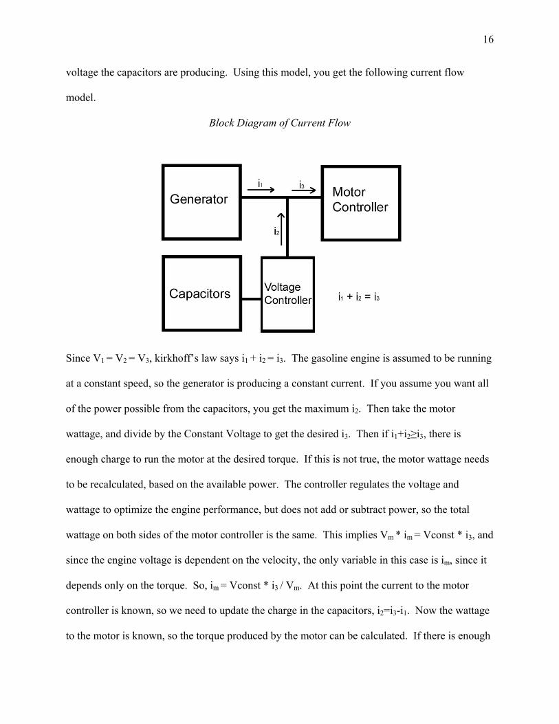
Block Diagram of Current Flow

Since V1 = V2 = V3, kirkhoff’s law says i1 + i2 = i3. The gasoline engine is assumed to be running

at a constant speed, so the generator is producing a constant current. If you assume you want all

of the power possible from the capacitors, you get the maximum i2. Then take the motor

wattage, and divide by the Constant Voltage to get the desired i3. Then if i1+i2≥i3, there is

enough charge to run the motor at the desired torque. If this is not true, the motor wattage needs

to be recalculated, based on the available power. The controller regulates the voltage and

wattage to optimize the engine performance, but does not add or subtract power, so the total

wattage on both sides of the motor controller is the same. This implies Vm * im = Vconst * i3, and

since the engine voltage is dependent on the velocity, the only variable in this case is im, since it

depends only on the torque. So, im = Vconst * i3 / Vm. At this point the current to the motor

controller is known, so we need to update the charge in the capacitors, i2=i3-i1. Now the wattage

to the motor is known, so the torque produced by the motor can be calculated. If there is enough

17

power in the system to drive the motor the torque is simply the desired torque, if there is a lack

of power, then torque must be recalculated using torque = kt * im.

At this point the hybrid system has been determined, but the actual performance of the

car is still unknown. In the most simplistic sense, a = mF . And the force applied is from the

torque applied to the wheel, or wheelradius

Torque . Add in aerodynamic drag, and some rolling

resistance, and you get an equation for acceleration in terms of torque, that we got from Steve

Hallowell’s Thesis, All Wheel Drive Utilizing Independent Torque Control of Each Wheel.

(kg)m

)(_)(_)()(

car

NmresistrollingNmdragaeromr

Nm

onAccelerati wheel−−

Τ

=

Here, the radius of the wheel is 0.25 m, and the aero drag is described by the following equation.

Faero= ))((*))((*))((*5.* 223 marea

smV

mkgdensityC frontalcaraird

Where the Cd, the coefficient of drag was estimated at .36, and the frontal area was estimated to

be .557m, and the density of air is 1.2929kg/m3. The rolling resistance was approximated at 10.

The mass of the car currently is 500lbs, and we would like the car to weigh in about the same

when we get done, so for the current run of the model, we used mcar = 320kg (500lbs for the car

plus 180lbs for the driver). As a side note, the MATLAB code models only one motor, so the

code used half weight, half generator input and half capacitor storage. From the acceleration it

was easy to calculate the velocity and the distance traveled using basic Newtonian physics.

V(t)=a*t+V0, and S(t)=a(t^2)/2+V*t+S0, where V0, and S0, are the velocity and position at the

previous point.

18

There is one over-simplification in the code that has yet to be explained, and that is the

charging/discharging efficiency of the ultracapacitors. Our full code is found in Appendix A.

The code assumes this efficiency is 100%, where in reality this efficiency is a function of time,

and the rate of charge. We have yet to analyze the ex the exact formula. It would seem

appropriate to model the ultracapacitors’ inefficiency as a small resistor, but we have yet to

determine the number of capacitors and thus the size of the resistor. Also, the focus at this stage

of the project is the acceleration event, which is hopefully less than 4.2 seconds long. There is

no charge/discharge cycle for that event, so the efficiency is not a large issue at this point. We

will continue to analyze the capacitor efficiency when modeling a sample drive cycle for the

endurance event.

Software Results

Below is a small set of results. Full results for several motor and generator sizes, and

extended distances are included in Appendix A. Here is the graph of the most likely results at

this stage in the process. All the graphs are done with a 200 N-m motor, and a 15 kW generator.

19

Here is the acceleration graph. The initial acceleration is not horizontal because of the

way the integration was approximated, with one value for every time step. It doesn’t start at zero

which is slightly confusing, but that stems from the graphing code. The time step in this case is

.05 seconds. As time goes on the acceleration goes down slightly due to aerodynamic drag. The

code runs on a distance-covered basis, so the accelerations stop when the car hits 75m rather than

at a given time interval so the higher accelerations stop before the slower cars. The Road and

Track data in black was only for 0-60 mph so it doesn’t quite extend as far as the calculated data.

With a gear ratio of 1:1, the motor was spinning at around 1200rpm at the end of the 75m

acceleration run. Since the motors that we looked at maxed out around 6000 rpms it seemed a

waste to have the engine spin at such a slow speed. The gear ratios in the figure are (motor rpm)

: (wheel rpm), so a higher number means the motor is spinning faster. The gear ratio goes only

to 2.5 because at 3, the motor was close to its maximum rpm at the end of the 75m. The higher

gear ratio produced a proportional increase in torque, and therefore acceleration, but it also

results in a proportional increase in the power used by the motor, since the voltage across the

20

motor is proportional to the angular velocity of the motor. The gear ratio of 2.5 shows the results

when the capacitors discharge fully. The available power drops drastically, so the acceleration

suffers. If the distance was extended the acceleration would not go to zero as the figure

indicates, it would bottom out at a slowly decreasing rate, as shown the figure below.

21

This is a graph of the charge in the capacitors. The coulombs are assuming a voltage of Vconst=182V. The first ten seconds where the charge grows linearly are the charging period. At ten seconds the motors rev-up. The curves get steeper as time progresses since the motor draws more power at higher rpms. Here it is obvious that the higher torque of the higher gear ratio comes at a price. In this case with a gear ratio of 2.5:1, the motor actually uses up all ten seconds worth of stored energy in the space of 75m.

These are the velocity curves, the gear ratio of 2.5 tails off at the end since due to the lack of power.

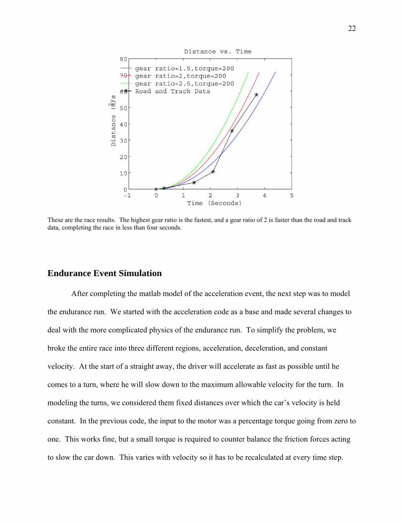
22

These are the race results. The highest gear ratio is the fastest, and a gear ratio of 2 is faster than the road and track data, completing the race in less than four seconds.

Endurance Event Simulation

After completing the matlab model of the acceleration event, the next step was to model

the endurance run. We started with the acceleration code as a base and made several changes to

deal with the more complicated physics of the endurance run. To simplify the problem, we

broke the entire race into three different regions, acceleration, deceleration, and constant

velocity. At the start of a straight away, the driver will accelerate as fast as possible until he

comes to a turn, where he will slow down to the maximum allowable velocity for the turn. In

modeling the turns, we considered them fixed distances over which the car’s velocity is held

constant. In the previous code, the input to the motor was a percentage torque going from zero to

one. This works fine, but a small torque is required to counter balance the friction forces acting

to slow the car down. This varies with velocity so it has to be recalculated at every time step.

23

We came up with a short algorithm that scaled the torque range up so that zero torque is the

amount of torque necessary to produce zero acceleration. To determine this torque, we went

back to Steve Hallowell’s formula governing acceleration based on torque and speed.

(kg)m

)(_)(_)()(

car

NresistrollingNdragaeromr

Nm

onAccelerati wheel−−

Τ

=

Solving this equation for torque when the acceleration equals zero produces the following

equation.

)(*))(_)(_()0(@ mrNresistrollingNdragaeroaccelTorque wheel−==

This is the new lowest value of the torque, but the torque should still be able to reach its

maximum. With a little linear interpolation, we came up with the following formula.

yAytorqueATorque ** −+=

Where, )0(@ == accelTorquey as given above, and A is the torque percentage input by

the user ranging from zero to one. In this case when A=0, all the A terms cancel out and torque

equals y, when A=1, then y-y=0, so torque=torque as desired.

24

This seems to work, but over long periods of time, what should be a constant line at

accel=0, falls gradually. It tends to be in the order of .1sm per 2 minutes, so it is not a big

problem, though it is slightly perturbing.

The velocity around the turns is fixed, but in between the turns, it’s a much more

complicated scenario. The straight-away starts with a period of intense acceleration, and finishes

with a period of deceleration stopping at the velocity ceiling of the next turn. There were several

ways to model the deceleration. The easiest way is to shut off the motors, and use the brakes to

slow the car down. In this case, the electronics would function exactly as in the charging phase,

with all the generator power running to the capacitors. This is how our sponsor specified we do

it. Braking an electric car without getting any sort of power back is negligent. The one true

performance advantage that electric cars have over gas is that they recycle some energy during

breaking. This process is called regenerative braking. It works exactly like a generator, the

momentum of the car spins the wheels, and the braking torque is created by drawing a large

current from the motor and into the capacitor bank. Regenerative breaking is beyond the scope

of our project, but we thought it would be interesting to approximate it and see how it affects the

race. To model regenerative braking, we modeled a forward acceleration of 1.2 times the

maximum torque, since braking should be quicker than acceleration. Taking this curve and

mirroring it about its center gives a deceleration curve. It also creates an increasing capacitor

charge curve. The motor current is divided by 2 to keep from over estimating the power of

regenerative braking. After the acceleration and deceleration curves are intersected, the

capacitor charge curve is moved so that it starts where the acceleration curve leaves off. It would

also work to make the acceleration negative, but having the turns on either end of the straight

away creates a boundary problem that is hard to solve with an initial value condition. Instead of

25

using an iterative method to solve this boundary condition problem, you can start at that final

velocity, accelerate and mirror the curve and end up at exactly the correct velocity to enter the

upcoming turn. Here is a graph of this process in action.

In this graph a. is the acceleration curve and b. is the acceleration curve to be mirrored.

Inv is b mirrored about its central axis. Aspl. and bspl. are matlab spline interpolations of the

data curves.

The mirroring eliminates the need to iterate for the velocity, but the intersection of the

two curves has to be determined. Now if they were mathematical functions, the intersection

would be easy to find. Since they are long arrays of numbers, it is not that simple. We tried to

write a program that compared all pairs of successive points between the two data sets to see if

the curves line intersected between them. After many hours of frustration and logical

26

quandaries, this approach proved fruitless. In its place we used a less elegant but more fool

proof method. We took each data set and interpolated a line though the points using a built in

matlab interpolating function. We were unable to find a way to automatically find the

intersection of the two points, but it is possible to evaluate the interpolating curve at any point.

This allowed us to use Newton’s Method to find to intersection.

Here’s small graph of a single straight-away with both the acceleration phase and the

deceleration phase.

This method has never failed to get a reasonable answer, though sometimes it is off by

one time step from the correct intersect which is normally .01 seconds. This is not a significant

27

error. Another problem with this method is that the data points for the acceleration and

deceleration are concatenated without interpolating the time where the deceleration starts. The

time interval is set to be one time step. This introduces some small error, but by reducing the

time step this error can be minimized. From the first term, we changed the end of the time step

iteration to be a set distance, rather than a time. This worked marvelously for the endurance run,

but since we didn’t interpolate to get the exact end value, there was is another error region that is

bounded within a time step. In all there are several small errors due to incomplete concatenation,

but they’re all bounded by a time step so they diminish as the time step shrinks.

We also wrote a program that draws a race track, and based on the radius of the turns

used to draw the track, calculates the constant velocity of each turn. Unfortunately we never got

any tire data, so we didn’t figure out the exact centrifugal force necessary for the car to spin out

when rounding a corner. As a ball park figure, we decided the maximum centrifugal acceleration

allowable is one G, or 9.81 2sm . Centrifugal force is defined as.

rmvF

2

=

Where F=ma. If a=9.81 2sm , then )

sm( 9.81* r*µ=v 2turn , where µ is the coefficient of

friction. Since the car runs racing slicks, the coefficient of friction was set to be .85.

28

Simulated Race Track

Here is the computer drawn track next to a picture Doug Fraser took of a past track. The track is

a little long, the straight-aways are mandated to be less than 75m in length, and the ones on the

computer drawing go up to 100m long.

Here are some of the results of the endurance run. We didn’t hone in one final motor

configuration so these test are run using a motor that puts out 250Nm of torque with a gear ration

of 2:1. We have settled on a generator that puts out around 30kW. Not surprisingly, the size of

the generator determines whether or not the capacitor bank discharges fully during the race. A

full discharge reduces the amount of power available for the motor and slows it down, which is

29

an undesirable occurrence on the race track. The 30kW generator more than enough even

without the benefits of regenerative braking.

The exciting part about this graph is the charge over time graph. The capacitor charge

increases over time. This means the car will never run out of charge. It will have the necessary

power whenever it needs it. The velocity curve shows the velocity spikes during the straight-

aways and the flat regions where the velocity is constant. The trouble we were having with the

constant velocity lines trailing off is apparent in this picture.

When the generator is downsized to 20kW’s the outcome is not as encouraging.

30

For most of the race, the capacitors are fully charged. In five places though, the capacitors are

fully discharged. This reduces the acceleration of the car as evidenced by the low level steps in

the otherwise rectangular sine wave curve.

There is a drastic difference when taking regenerative braking into account. Even with

the 50% inefficiency rating we programmed in, the regenerative braking system requires a

generator that is only half the size of the non-regenerative system.

31

This graph is for a 15kW generator, the increasing capacitor charge is reminiscent of the 30kW

non-regenerative system.

This last set of charge and velocity graphs are using only a 10kW generator. Again there is not

quite enough power in this system. The end charge is far higher than the starting charge, so this

could work out if the car is fast enough to overcome a slow start. Though going with a larger

generator would be the best solution.

These results are very encouraging. The acceleration tests showed that the hybrid race

car is strong enough to win over short distances, but the endurance run graphs show that the

balance of power between the motors and the generator is sufficient to race the car for extended

periods of time.

32

Test Prototype Simulation

The only piece missing from these results is a real world corroboration of the

mathematical conclusions. In this vein, we built a scaled down test bed, which consists of one

motor, a generator and a bank of capacitors. We will go into far more detail about the

construction of the test bed later in the report. To compare the computer results to the test bed,

we tailored the earlier code to match inputs from the test bed. We took out the percentage torque

input and used the desired torque as an input criterion so we could mirror what the torque meter

was reading. We removed all the motion equations and focused on motor dynamics and current

flow. One of the major points that was not addressed in the previous models was the actual

behavior of the capacitors under loading. In the previous models, we assumed a voltage

controller would equalize the capacitor voltage so that it was always a constant. In the test bed

we did not have this piece of equipment, so the whole system ran at the capacitor voltage level.

A motor controller and a large inductor controlled the voltage from the generator. On the motor

side, since the motor controllers are only down converters, the maximum engine rpm was

determined by the capacitor charge. This means as the capacitors discharge, the engine turns

slower and draw less power, which means the capacitor voltage is very important in the

modeling. On Maxwell’s website they have a guide to sizing your own ultracapacitor bank that

includes a brief look at the equations involved.

(http://www.maxwell.com/ultracapacitors/support/app_notes/general_sizing.html)

They state that constant voltage discharge has two governing components, the capacitance and

resistance. The capacitance is define as dtdVCi *= , and the resistive component is governed by

the equation V=i*R. Combine those two equations and you get RiCdtidV **

+= . Now our

33

model will be taking a number of incremented measurements, so i*R will be added up a varying

number of times depending on the time step. So we chose to use the change in resistivity rather

than the total or ∆V=∆i*R, so that CdtidV *

= + ∆i*R.

Armed with this information, and some good motor characteristics for the motors in our

test be we rewrote a section of code to mimic the test bed.

The graphs came out nicely with a long charging time for the capacitors. The voltage

curves have a quick jump at the beginning that is due to the resistivity of the ultracapacitors, and

34

the motor current and the generator current even out over time. The capacitor bank controls the

voltage, so the only equilibrium point remaining is current and the two stabilize so there is no net

charge in the state of charge of the ultracapacitors. Also the graph lines up nicely with this

explanatory graph from the same Maxwell webpage.

Where esr is the resistive element, Vw is the working voltage. This graph has a linear discharge

rate because the current draw is constant. In the test bed as the voltage goes the motor spins

slower and draws less power. As the motor draw decreases, the capacitors need to supply less

and less power to step the generator current up to that of the motor.

35

Investigation of Formula SAE Drive Cycles

Our drive cycle specifications for the acceleration test are simple: from rest, accelerate as

fast as possible for 75 meters. We’ve specified 4 seconds as the goal time for our system, since

we think that time will win the competition.

Although it’s easy to say “step on the gas for 75 meters,” it’s another thing to model it

and find out how a car will perform. Dynamometer charts from Formula SAE cars are hard to

come by, and actual Formula SAE results aren’t very descriptive—they provide each team’s

acceleration time, but no intermittent data. In addition, driving strategies affect acceleration

time: by revving the engine before accelerating, drivers essentially spin a flywheel and quickly

put the car in gear, transferring the kinetic energy from the flywheel to the wheels. This gives

the car good acceleration at the start. Road and Track magazine invited the top five teams from

the 2002 FSAE to its own competition, which included an acceleration test for 0-60 mph times.

All teams used a 600 cc motorcycle engine. They reported the time each team took to reach each

10 mph increment. The best team, which also had the most representative acceleration, was

Lawrence Technical University, which also implemented a turbocharged engine:

Lawrence Technical University Acceleration Data

Lawrence Technical University

0-10 mph 0-20 mph 0-30 mph 0-40 mph 0-50 mph 0-60 mph

Time (seconds) 0.3 0.8 1.4 2.1 2.8 3.7

36

Acceleration vs. Time (Lawrence)

0

5

10

15

20

0 1 2 3 4time (seconds)

acce

lera

tion

(m/s

^2)

Full results from the competition, as well as velocity vs. time and distance vs. time

graphs, can be found in Appendix B. We can use this data to estimate the acceleration of

competing cars, and we’ve compared our model to these results to see how we measure up.

Since our proposal, our sponsor has asked us to also consider the drive cycle for the

endurance event. Although there is no standardized racecourse for upcoming events, Formula

SAE specifies certain guidelines (http://www.sae.org/students/fsaerules.pdf) for the endurance

course (speed guidelines are for course construction and general prediction only—cars go as fast

as they safely can over the entire course):

Average speed: 48 – 57 km/hr (30 - 35 mph)

Top speed: 105 km/hr (65 mph)

Straights: < 77 m with hairpins at both ends

< 61 m with wide turns at ends

37

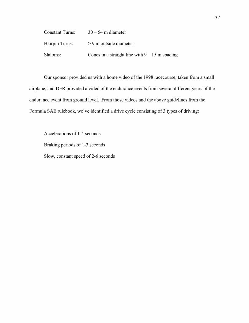
Constant Turns: 30 – 54 m diameter

Hairpin Turns: > 9 m outside diameter

Slaloms: Cones in a straight line with 9 – 15 m spacing

Our sponsor provided us with a home video of the 1998 racecourse, taken from a small

airplane, and DFR provided a video of the endurance events from several different years of the

endurance event from ground level. From those videos and the above guidelines from the

Formula SAE rulebook, we’ve identified a drive cycle consisting of 3 types of driving:

Accelerations of 1-4 seconds

Braking periods of 1-3 seconds

Slow, constant speed of 2-6 seconds

38

Endurance Track

Digital image taken from Doug Fraser’s 1998 DFR video

Work Accomplished: Test Prototype

Most of our work in the second term of this project has been on constructing a test

prototype. We have succeeded in selecting and purchasing all components, as well as

assembling the system on a table for testing. We also configured our system to attach to a torque

meter and dynamometer, but due to time constraints and equipment problems we failed to collect

any relevant test data. Below is outlined our selection process for each component, our design

process for creating the test prototype, and pictures of our assembled system.

39

Component Selection

Since our system has many integrated parts, each component had to fit within the overall

system requirements as well as individual specifications. Because some components are more

flexible than others, we chose to begin with a feasible motor, then found an engine-generator

combination. Only after that did we select the size and characteristics of our ultracapacitor bank.

Finally, we chose motor controllers to interact between all components.

Electric Motor

Although at first we thought we wanted a brushless DC motor for its efficiency and low

maintenance, we realized that brushless motors are much more expensive, and harder to control.

We decided to move to a brushed DC motor since they are reasonable reliable (though the

brushes can wear out after much use), and there are most “amateur” electric vehicle enthusiasts

use brushed DC systems. We researched state of the art, and finally settled on the Briggs and

Stratton Etek motor, since it is very popular, lightweight, inexpensive, and in the size range we

wanted (48 V). Etek motor information can be found in Appendix C. In addition, since it was

such a good fit, we purchased two motors, and used one for our generator.

Ultracapacitor Storage System

To determine the size of our capacitor bank, we used the expected peak power from the

motor and the motor’s efficiency:

input power efficiency

routputpowe=

40

Knowing that we need an expected input power of 17 kW (23 hp) for 4 seconds (4

seconds of peak power to the motor) and an input voltage of 48 Volts, we apply the following

equation:

( )( )2

2CVtimepowerE ==

We get a capacitance of 59 F. Maxwell ultracapacitors are rated at 2.5 V, so 20

capacitors in series gives us 50 V. Putting the capacitors in series has an inverse effect on the

total capacitance. For a total capacitance of 59 F, each capacitor must be rated at 1180.

However, this assumes that we expect to discharge the ultracapacitors fully each time we

accelerate, which would be foolish since the voltage would drop to zero and there would be no

power to the wheels by the end of the 4 seconds. After further research, we used Maxwell’s

ultracapacitor modeling system (Appendix D) to find a solution that fit our needs. This

Microsoft Excel program takes into account the initial resistance drop of the ultracapacitors, a

linear charge drop, and a “bounce back” characteristic once the load has been removed (We

observed this characteristic ourselves by charging the capacitors, discharging them, and watching

the voltage climb a few volts after the discharge). Maxwell’s program gave us a much more

reasonable answer of a 90 Farad system. After speaking with a Maxwell representative, we

decided to go instead with a 135 Farad system (20 by 2700 Farads), since their larger, older

capacitors were at an education discount price. This also meant our minimum voltage would be

only 32 V, giving us greater power throughout the 4 seconds. See Appendix E for complete

specifications on our capacitors.

41

Internal Combustion Engine / Generator

At first, we expected to use a small motorcycle engine to power our generator. However,

building the test prototype required us to give up lightweight, efficient components and replace

them with cheaper, simpler, more readily available elements. With this in mind, we purchased a

5.5 hp Briggs and Stratton engine to be coupled with our second Etek motor. We chose a 5.5 hp

engine since that rating agreed closely with both the motor’s continuous rating and the size of the

ultracapacitor bank. The generator should be able to charge the entire capacitor bank in about 40

seconds.

Although we originally assumed we would have a smaller motor for our generator, we

eventually realized that the generator must run at the motor’s continuous power rating (or lower),

while the drive train motor should be sized for peak power. Therefore, we used one of our Etek

motors as the generator for our system.

Motor Controllers

We have two motor controllers in our system: once controls the power going into the

ultracapacitors, and the other controls the power going into the drive motor. Curtis Instruments

manufactures motor controllers for electric vehicle use, and many “rebuilt” Curtis controllers are

available. We purchased two of these rebuilt controllers (1204 and 1206), sized for our needs,

since they are at a reduced price. Although they are meant for a battery input and motor output,

we adapted them for use with our system.

42

Design/Assembly Process

Designing and building the actual test prototype took much more time and money than

expected. We designed everything in Pro Engineer before building it in the machine shop and

mounting it on our test bench.

Dynamometer:

First, we salvaged Dartmouth Formula Racing’s old dynamometer from the DFR trailer.

Although it was dirty and needed some work, it provided the braking power we needed to test the

torque from our motor. Old DFR team members had never been able to measure torque with it,

so we used it only as a load on the motor, and planned to measure torque with a separate torque

meter. The dynamometer also utilizes a water pump with a control valve, to adjust the load on

the shaft.

Motor Mounts and Couplings:

Since our motors have only face mounts, we machined and welded two motor mounts,

each at appropriate heights for coupling with the engine and dynamometer. We also purchased a

43

Lovejoy coupling set for the engine/generator, to transfer power between the shafts. For the

motor/dynamometer connection, we placed a torque meter between the two shafts, and since the

torque meter already had two Browning couplings we bought two more (for 2 complete sets)

couples and two rubber inserts. We then measured the height of the shafts, lengths of the shafts,

and locations of mounting holes, and finally drilled matching holes in our table to mount the

engine, generator, drive motor, and dynamometer.

Ultracapacitors:

Ultracapacitors in series must use voltage balancing to regulate current flow between

capacitors and ensure that each capacitor has the same voltage at all times. To do this, we

ordered voltage balancing kits from Maxwell Technologies and assembled the capacitor bank

and voltage balancing circuits. Once this was complete, we shorted the end terminals together

(to keep the capacitors discharged) and placed them in a wooden box with a Plexiglas cover.

Since the ultracapacitors represented the biggest safely risk, it was important to protect them

from unnecessary tampering and accidental shorting.

44

Inductor:

Since ultracapacitors’ voltage varies with state of charge, it is necessary when charging

them to begin by applying a low voltage and slowly increase it. However, Curtis motor

controllers regulate power not by adjusting voltage, but by changing it to a square wave and

varying the duty cycle. Magdalena Dale designed a large inductor (33 µH) for our system to

smooth the output and charge the capacitors.

Wiring and Circuit:

Once all of the “minor” components were in place, we designed our circuit using AWG

#2 welding cable for our high current connections. We placed large fuses in series with the

capacitors and with the generator to protect the system in the event of a short circuit. We also

used a contactor with each controller open and close the circuit. The entire circuit can be found

in Appendix G.

45

Final Prototype

Additional photos and renderings can be found in Appendix H.

46

Analysis of Full-sized System

Electric Motor

To identify a power and torque range for the motor we needed, we used an equation

relating acceleration to torque:

amrT ××=

T = torque of wheel axle (N-m) m = mass of car (kg)

r = radius of wheel (m) a = acceleration (m/s2)

A constant acceleration of 9.4 m/s2 will give us a time of 4 seconds for a 75 meter course,

with a top speed of 88 mph. Using a car mass of 308 kg (680 lbs, including driver) and a wheel

radius of .25 m (10 in), we get a torque value of 724 N-m. Split into two motors (one for each

rear wheel), each motor should have a peak torque rating of 362 N-m. While this is a higher

value than we initially expected, it is feasible with current state of the art.

Because of the characteristics of electric motors, a constant acceleration can be expected.

Electric motors have a constant torque up to a certain rotational speed, at which point it drops

off. Thus, the motor’s power (hp = Tω) increases linearly to that rotational speed, then stays

constant before dropping off also. For comparison, below are a torque curve from DFR’s current

Yamaha 600 cc engine and a performance chart from our Etek motor. While it is difficult to

compare the different axes, you can see that the Yamaha engine has zero torque at zero rpm, and

doesn’t achieve maximum torque until about 9500 rpm.

47

http://www.motorcycle.com/mo/mccompare/01600/mcphotos/01yzfr6dyno.html

48

The motors of choice for electric vehicle drag race enthusiasts seem to be either Kostov

fork-lift motors or Advanced DC motors. Both are very powerful and come in a variety of sizes.

We’ve identified the Advanced DC L91-4003 motor as most feasible for a full-scale system.

Specifications are in Appendix I.

Capacitor Storage System

We’ve identified ultracapacitors as the most viable solution to storing electrical energy.

Ultracapacitors have a weaker energy density than batteries, but a greater power density,

meaning the ultracapacitors can discharge and provide lots of energy very quickly.

Ultracapacitors also have a much longer cycle life than batteries, and aren’t damaged by

incomplete charging and discharging. These are all important considerations for our system,

since we need an energy storage bank capable of responding to our needs at any specific time. If

we have extra energy, we want to store it in the bank, even if it’s already mostly full. If we need

all the energy we have, we want it very quickly so we can accelerate the racecar.

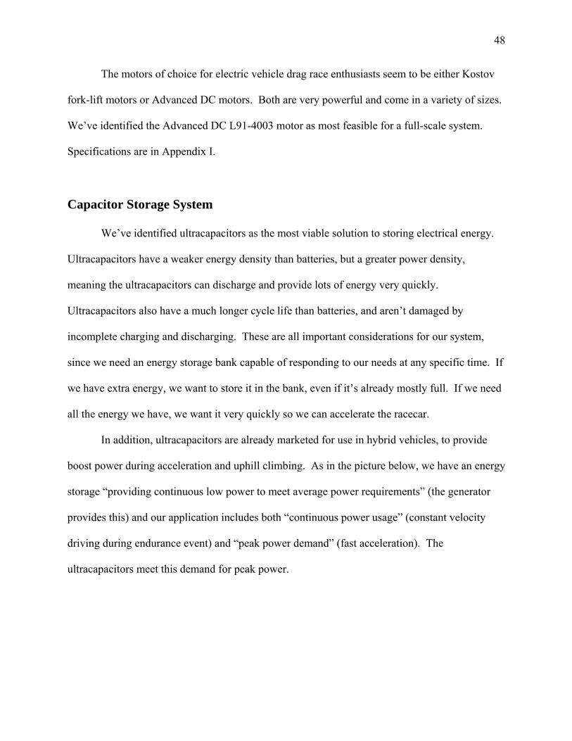
In addition, ultracapacitors are already marketed for use in hybrid vehicles, to provide

boost power during acceleration and uphill climbing. As in the picture below, we have an energy

storage “providing continuous low power to meet average power requirements” (the generator

provides this) and our application includes both “continuous power usage” (constant velocity

driving during endurance event) and “peak power demand” (fast acceleration). The

ultracapacitors meet this demand for peak power.

49

http://www.maxwell.com/ultracapacitors/support/overview.html

As in our test prototype, we used Maxwell’s ultracapacitor modeling system to determine

our power needs, and we calculated that we need 48 ultracapacitors in series for a 120 V system.

Each capacitor is 2700 Farads, which results in a 56 Farad capacitance, and 400 kJ of total

energy available. A storage system of this size weighs 75 lbs and costs about $2700, including

voltage balancing kits.

Internal Combustion Engine / Generator

We expect to use a small gasoline-powered motorcycle engine to provide the power to

charge the ultracapacitor bank and to contribute power to the electric motors. Yamaha 125 cc

and 250 cc dynamometer charts are shown below, indicating little difference in performance.

Since the 125 cc engine in cheaper and lighter, we would select it to turn our generator.

50

Yamaha YZ125 SST

http://www.fmfracing.com/dynoroom.asp

51

Motor Controllers

The Zilla Z1K motor controller is rated at 72-156 V, and 1000 Amps (maximum). Two

of these controllers (one for each motor) would work for our system, which would operate at 120

V and a maximum of 600 Amps. These controllers are extremely flexible and can easily work

with our system. In addition, we will need another smaller controller, such as a Curtis controller,

for the generator. It also might be possible to control the voltage to the capacitors by directly

varying the speed of the generator, in which case a controller may not be necessary. The control

aspect of the capacitor charging has the most potential for future work, and an efficient, semi-

autonomous charging system would be very useful and innovative.

Overall weight and cost analysis

Component Cost Weight

Motors $1600 170 lbs

Controllers $3500 40 lbs

Ultracapacitors $2400 75 lbs

Engine/Generator $2000 80 lbs

Total $9500 365 lbs

Although a hybrid Formula SAE racecar is certainly within the realm of current state of

the art, the cost and weight specifications will not be met. The subtracted items (Yamaha 600 cc

engine and differential) combined weigh only 160 lbs, so we would have a net gain of 200 lbs.

This would increase the mass of the car, requiring larger motors and more capacitors. Therefore,

52

our recommendation is to not move to a hybrid racecar without much further research and

testing.

53

Works Cited

Blindheim, David N., 290 Final Written Report, March 4 2003, unprinted. Hallowell, Stephen J., All Wheel Drive Utilizing Independent Torque Control of Each Wheel. Senior Honors Thesis, Thayer School of Engineering, June 5, 2001. http://wave.prohosting.com/sunwater/hybrid.html

http://www.ott.doe.gov/hev/

http://www.drivesmag.com/Articles/Pitt_Tube/AC_vs_DC.html http://www.joliettech.com/adjustable_speed_drives-application_information.htm http://www.galco.com/circuit/brakecontrol.htm http://www.cloudelectric.com/generic.html?pid=66 http://www.premag.com/products/products.htm

http://www.baldor.com/

http://www.motorcycle.com/mo/mccompare/01600/mcphotos/01yzfr6dyno.html http://www.bbrmotorsports.com/Stock.htm

Updated Timeline

Original Timeline

The code that analysis the car performance. function T = RunCycle4(s,g,m,del) % all values are for half of a car % each half is driven by one motor, half of a generator, half of an engine, % and half of the total capacitor bank. delta=del; % seconds save delta %When changing delta, change generator function as well. maximum_torque=m; % N-m maximum_rpm=6000; torque_graph=MakeUpTorque(maximum_torque,maximum_rpm); wheel_radius=.25; % meters mass_car=160; % kg (half of car) Vconst=182; % Voltage of motors R=3; % V = ke*omega + R*i kt=3.77; % i = (1/kt)*tau ke=2.18; % V = ke*omega + R*i gear_ratio=g; % from "gearing.m" probably 2:1 save maximum_torque save maximum_rpm save torque_graph save maximum_engine_draw save engine_voltage save wheel_radius save mass_car save Vconst save gear_ratio len=length(s(:,1)); its=1; % incremental counter caparray(its)=0; cap=0; A(its)=0; % acceleration V(its)=0; % velocity S(its)=0; % position its=2; Ath(1)=A(1); % unlimited capacitors Vth(1)=V(1); % " Sth(1)=S(1); % " i3array(1)=0; % amperage to the motor controller totalcount=0;

%Charging phases, this is in time, not distance convered. for i=1 a=s(i,1); % initial inputs, exception for j=0:delta:s(i,2) % input is [acc, dist covered for that acc] x=Generator+cap; % x is available amperage, cap is charge in capacitors % Generator is amperage that generator % produces (constant) m=Motor(a,V(its-1),x,R,kt,ke,delta); % Motor returns acc [m(1)] and % amperage [m(2)] that motor draws. cap=-m(2)+Generator+cap; % update cap charge i3array(its)=m(2); % stores motor's amperage draw caparray(its)=cap; % stores cap charge over time % store Acc, Vel, and Dist over time to graph later A(its)=m(1); V(its)=A(its)*delta+V(its-1); S(its)=A(its)*delta^2/2+V(its)*delta+S(its-1); % does same thing again, with unlimited capacitance m=Motor(a,Vth(its-1),Vconst*maximum_torque,R,kt,ke,delta); Ath(its)=m(1); Vth(its)=Ath(its)*delta+Vth(its-1); Sth(its)=Ath(its)*delta^2/2+Vth(its)*delta+Sth(its-1); its=its+1; end end % same as last big loop, only it's a function of distance covered % rather than time for i=2:len a=s(i,1); dist=0; while (dist<s(i,2)) x=Generator+cap; m=Motor(a,V(its-1),x,R,kt,ke,delta); cap=-m(2)+Generator+cap; i3array(its)=m(2); caparray(its)=cap; A(its)=m(1); V(its)=A(its)*delta+V(its-1);

S(its)=A(its)*delta^2/2+V(its)*delta+S(its-1); dist=A(its)*delta^2+V(its)*delta+dist; m=Motor(a,Vth(its-1),Vconst*maximum_torque,R,kt,ke,delta); Ath(its)=m(1); Vth(its)=Ath(its)*delta+Vth(its-1); Sth(its)=Ath(its)*delta^2/2+Vth(its)*delta+Sth(its-1); its=its+1; end final(i-1)=(its-1)*delta-s(1,2); end % %%%%%%%%% graphs - all graphs are over time %%%%%%%%%%%% % These plots are for individual results when not using Gearing.m % figure % subplot(2,3,1) % plot((1:its-1)*delta,Ath,'m',(1:its-1)*delta,A,'g') % acceleration over time % hold on % plot([.15,.55,1.1,1.75,2.45,3.25]+s(1,2),[14.9,8.94,7.45,6.38,6.38,4.97],'k*-') % % plot data from road and track % % hold off % legend('Accel-Best','Accel-Limit') % subplot(2,3,2) % plot((1:its-1)*delta,Vth,'r',(1:its-1)*delta,V,'k') % Velocity % legend('Vel-Best','Vel-Limit') % subplot(2,3,3) % plot((1:its-1)*delta,Sth,'g',(1:its-1)*delta,S,'b') % distance % hold on % plot([0,.3,1.4,2.1,2.8,3.7]+s(1,2),[0,.67,4.02,10.73,35.76,57.89],'k*-') % % road and track data % hold off % legend('Dist-Best','Dist-Lim') % subplot(2,3,4) % plot((1:its-1)*delta,caparray,'m') % cap charge % legend('Capacitor Charge') % subplot(2,3,5) % plot((1:its-1)*delta,i3array,'b') % amperage to motor controller % legend('i3') % subplot(2,3,6) % plot((1:its-1)*delta,V*(1+.03)/.25*gear_ratio) % angular velocity % legend('omega') T=[A;V;caparray;(1:its-1)*delta;S]; % return acc, vel, and cap charge values into "gearing.m"

function M = Motor(A,v,ig,R,kt,ke,h) load mass_car load torque_graph load wheel_radius load maximum_rpm load gear_ratio load engine_voltage load Vconst; if(v<0) % stipulations for negative or zero velocity error('Car has slowed beyond a stop'); elseif((v==0)&(A==0)) M=[0,0]; %This is for when the capacitor's are charging and the car is stopped %in this case the motors are not on. else Cd=.36; % drag coefficient, unitless fa=.557; % frontal area, in m^2 rpm=v*(1+.03)*60/(2*pi*.25)*gear_ratio; %Calculates the motors rpm, using a %using a slip percentage of .04 omega=rpm*2*pi/60; %Angular velocity f=floor(rpm); % integer value of rpm if(f>maximum_rpm) trq=torque_graph(maximum_rpm) % shouldn't ever happen (at max speed, % there is zero torque, so no % acceleration) else trq=torque_graph(f+1); end trq=A*trq; % A is percent acceleration desired (usually A = 1) im=1/kt*trq; % motor amperage over a one second interval Vm=ke*omega+R*im; % motor voltage if((ig*Vconst/h)>(Vm*im)) %ig is over delta, Vm over one second, so need to equalize the time frame i3=(Vm*im)/Vconst; % Decide if you have enough current available % if so, use that current here else im=ig*Vconst/(Vm*h); % if not, use max current available i3=ig/h; trq=kt*im; end

trq=trq*gear_ratio; % new torque taking account of the gear ratio Am=(trq/wheel_radius - aero_resistence(Cd,v,fa)-10)/mass_car; % acceleration based on mass, torque, % wheel size, from Steve Hallowell's % equation M=[Am,i3*h]; %Returns, [Acceleration,Amperage required] end %%%%%%%%%%%%%%%%%%%%%%%%%%%%%%%%%%%%%%%%%%% function G = Generator load delta load Vconst G=15000*delta/Vconst; %Assume a 30KW Generator, coulombs per delta

The program used to graph the results obtained in RunCylce5 function T = Gearing close all; ctime=10; %Charge time in seconds del=.05; %Time step in Seconds s=([0,ctime;1,75]); g=1; m=100; %Motor torque= 150Nm aa=RunCycle5(s,g*1.5,m*1.5,del); a=RunCycle5(s,g*2,m*1.5,del); b=RunCycle5(s,g*2.5,m*1.5,del); %Motor torque=200Nm c=RunCycle5(s,g*1.5,m*2,del); d=RunCycle5(s,g*2,m*2,del); dd=RunCycle5(s,g*2.5,m*2,del); %Motor torque=300Nm d1=RunCycle5(s,g*1.5,m*3,del); d2=RunCycle5(s,g*2,m*3,del); d3=RunCycle5(s,g*2.5,m*3,del); %Motor torque=250Nm e=RunCycle5(s,g*1.5,m*2.5,del); f=RunCycle5(s,g*2,m*2.5,del); g=RunCycle5(s,g*2.5,m*2.5,del); %%Each of the four following figure, Acceleration, Distance, Cap Charge, %%Velocity, all take data from the above RunCycle5 runs aa through g, it %%plots each set of data on four seperate graphs, one for each motor torque %%with each three gear ratio's overlayed on the road and track data. %%%%%%%%%%%%%%%%Acceleration Graphs %%%%%%%%%%%%%%% figure t=1; %1=Acceraltion data subplot(2,2,1) plot(aa(4,ctime/del+del:length(aa))-s(1,2)-del,aa(t,ctime/del+del:length(aa)),a(4,ctime/del+del:length(a))-s(1,2)-del,a(t,ctime/del+del:length(a)),'r',b(4,ctime/del+del:length(b))-s(1,2)-del,b(t,ctime/del+del:length(b)),'g') xlabel('Time(Seconds)') ylabel('Acceleration(m/s^2)')

title('Acceleration vs. Time') hold on plot([.15,.55,1.1,1.75,2.45,3.25],[14.9,8.94,7.45,6.38,6.38,4.97],'k*-') legend('gear ratio=1.5,torque=150','gear ratio=2,torque=150','gear ratio=2.5,torque=150','Road and Track Data',0) legend boxoff subplot(2,2,2) plot(c(4,ctime/del+del:length(c))-s(1,2)-del,c(t,ctime/del+del:length(c)),d(4,ctime/del+del:length(d))-s(1,2)-del,d(t,ctime/del+del:length(d)),'r',dd(4,ctime/del+del:length(dd))-s(1,2)-del,dd(t,ctime/del+del:length(dd)),'g') xlabel('Time(Seconds)') ylabel('Acceleration(m/s^2)') title('Acceleration vs. Time') hold on plot([.15,.55,1.1,1.75,2.45,3.25],[14.9,8.94,7.45,6.38,6.38,4.97],'k*-') legend('gear ratio=1.5,torque=200','gear ratio=2,torque=200','gear ratio=2.5,torque=200','Road and Track Data',0) legend boxoff subplot(2,2,4) plot(d1(4,ctime/del+del:length(d1))-s(1,2)-del,d1(t,ctime/del+del:length(d1)),d2(4,ctime/del+del:length(d2))-s(1,2)-del,d2(t,ctime/del+del:length(d2)),'r',d3(4,ctime/del+del:length(d3))-s(1,2)-del,d3(t,ctime/del+del:length(d3)),'g') xlabel('Time(Seconds)') ylabel('Acceleration(m/s^2)') title('Acceleration vs. Time') hold on plot([.15,.55,1.1,1.75,2.45,3.25],[14.9,8.94,7.45,6.38,6.38,4.97],'k*-') legend('gear ratio=1.5,torque=300','gear ratio=2,torque=300','gear ratio=2.5,torque=300','Road and Track Data',0) legend boxoff subplot(2,2,3) plot(e(4,ctime/del+del:length(e))-s(1,2)-del,e(t,ctime/del+del:length(e)),f(4,ctime/del+del:length(f))-s(1,2)-del,f(t,ctime/del+del:length(f)),'r',g(4,ctime/del+del:length(g))-s(1,2)-del,g(t,ctime/del+del:length(g)),'g') xlabel('Time(Seconds)') ylabel('Acceleration(m/s^2)') title('Acceleration vs. Time')

hold on plot([.15,.55,1.1,1.75,2.45,3.25],[14.9,8.94,7.45,6.38,6.38,4.97],'k*-') legend('gear ratio=1.5,torque=250','gear ratio=2,torque=250','gear ratio=2.5,torque=250','Road and Track Data',0) legend boxoff %%%%%%%%%%%%%% Distance Graphs %%%%%%%%%%%%%%%%%%% figure t=5; %5=Distance data subplot(2,2,1) plot(aa(4,ctime/del+del:length(aa))-s(1,2)-del,aa(t,ctime/del+del:length(aa)),a(4,ctime/del+del:length(a))-s(1,2)-del,a(t,ctime/del+del:length(a)),'r',b(4,ctime/del+del:length(b))-s(1,2)-del,b(t,ctime/del+del:length(b)),'g') xlabel('Time (Seconds)') ylabel('Distance (m/s^2)') title('Distance vs. Time') hold on plot([0,.3,1.4,2.1,2.8,3.7],[0,.67,4.02,10.73,35.76,57.89],'k*-') legend('gear ratio=1.5,torque=150','gear ratio=2,torque=150','gear ratio=2.5,torque=150','Road and Track Data',0) legend boxoff subplot(2,2,2) plot(c(4,ctime/del+del:length(c))-s(1,2)-del,c(t,ctime/del+del:length(c)),d(4,ctime/del+del:length(d))-s(1,2)-del,d(t,ctime/del+del:length(d)),'r',dd(4,ctime/del+del:length(dd))-s(1,2)-del,dd(t,ctime/del+del:length(dd)),'g') xlabel('Time (Seconds)') ylabel('Distance (m/s^2)') title('Distance vs. Time') hold on plot([0,.3,1.4,2.1,2.8,3.7],[0,.67,4.02,10.73,35.76,57.89],'k*-') legend('gear ratio=1.5,torque=200','gear ratio=2,torque=200','gear ratio=2.5,torque=200','Road and Track Data',0) legend boxoff subplot(2,2,4) plot(d1(4,ctime/del+del:length(d1))-s(1,2)-del,d1(t,ctime/del+del:length(d1)),d2(4,ctime/del+del:length(d2))-s(1,2)-del,d2(t,ctime/del+del:length(d2)),'r',d3(4,ctime/del+del:length(d3))-s(1,2)-del,d3(t,ctime/del+del:length(d3)),'g') xlabel('Time (Seconds)')

ylabel('Distance (m/s^2)') title('Distance vs. Time') hold on plot([0,.3,1.4,2.1,2.8,3.7],[0,.67,4.02,10.73,35.76,57.89],'k*-') legend('gear ratio=1.5,torque=300','gear ratio=2,torque=300','gear ratio=2.5,torque=300','Road and Track Data',0) legend boxoff subplot(2,2,3) plot(e(4,ctime/del+del:length(e))-s(1,2)-del,e(t,ctime/del+del:length(e)),f(4,ctime/del+del:length(f))-s(1,2)-del,f(t,ctime/del+del:length(f)),'r',g(4,ctime/del+del:length(g))-s(1,2)-del,g(t,ctime/del+del:length(g)),'g') xlabel('Time (Seconds)') ylabel('Distance (m/s^2)') title('Distance vs. Time') hold on plot([0,.3,1.4,2.1,2.8,3.7],[0,.67,4.02,10.73,35.76,57.89],'k*-') legend('gear ratio=1.5,torque=250','gear ratio=2,torque=250','gear ratio=2.5,torque=250','Road and Track Data',0) legend boxoff %%%%%%%%%%%%%%%%% Capacitor Graphs %%%%%%%%%%%%%%%% figure t=3; %3=Capacitor Charge data subplot(2,2,1) plot(aa(4,:),aa(t,:),a(4,:),a(t,:),'r',b(4,:),b(t,:),'g') xlabel('Time (Seconds)') ylabel('Charge (Coloumbs)') title('Charge vs. Time') hold on legend('gear ratio=1.5,torque=150','gear ratio=2,torque=150','gear ratio=2.5,torque=150',0) legend boxoff subplot(2,2,2) plot(c(4,:),c(t,:),d(4,:),d(t,:),'r',dd(4,:),dd(t,:),'g') xlabel('Time (Seconds)') ylabel('Charge (Coloumbs)') title('Charge vs. Time') hold on legend('gear ratio=1.5,torque=200','gear ratio=2,torque=200','gear ratio=2.5,torque=200',0) legend boxoff

subplot(2,2,4) plot(d1(4,:),d1(t,:),d2(4,:),d2(t,:),'r',d3(4,:),d3(t,:),'g') xlabel('Time (Seconds)') ylabel('Charge (Coloumbs)') title('Charge vs. Time') hold on legend('gear ratio=1.5,torque=300','gear ratio=2,torque=300','gear ratio=2.5,torque=300',0) legend boxoff subplot(2,2,3) plot(e(4,:),e(t,:),f(4,:),f(t,:),'r',g(4,:),g(t,:),'g') xlabel('Time (Seconds)') ylabel('Charge (Coloumbs)') title('Charge vs. Time') hold on legend('gear ratio=1.5,torque=250','gear ratio=2,torque=250','gear ratio=2.5,torque=250',0) legend boxoff %%%%%%%%%%%%%% Velocity Graphs %%%%%%%%%%%%%%%% figure t=2; %2=Velocity data subplot(2,2,1) plot(aa(4,ctime/del+del:length(aa))-s(1,2)-del,aa(t,ctime/del+del:length(aa)),a(4,ctime/del+del:length(a))-s(1,2)-del,a(t,ctime/del+del:length(a)),'r',b(4,ctime/del+del:length(b))-s(1,2)-del,b(t,ctime/del+del:length(b)),'g') xlabel('Time (Seconds)') ylabel('Velocity (m/s^2)') title('Velocity vs. Time') hold on plot([0,.3,.8,1.4,2.1,2.8,3.7],[0,4.47,8.94,13.41,17.88,22.35,26.82],'k*-') legend('gear ratio=1.5,torque=150','gear ratio=2,torque=150','gear ratio=2.5,torque=150','Road and Track Data',0) legend boxoff subplot(2,2,2) plot(c(4,ctime/del+del:length(c))-s(1,2)-del,c(t,ctime/del+del:length(c)),d(4,ctime/del+del:length(d))-s(1,2)-del,d(t,ctime/del+del:length(d)),'r',dd(4,ctime/del+del:length(dd))-s(1,2)-del,dd(t,ctime/del+del:length(dd)),'g') xlabel('Time (Seconds)')

ylabel('Velocity (m/s^2)') title('Velocity vs. Time') hold on plot([0,.3,.8,1.4,2.1,2.8,3.7],[0,4.47,8.94,13.41,17.88,22.35,26.82],'k*-') legend('gear ratio=1.5,torque=200','gear ratio=2,torque=200','gear ratio=2.5,torque=200','Road and Track Data',0) legend boxoff subplot(2,2,4) plot(d1(4,ctime/del+del:length(d1))-s(1,2)-del,d1(t,ctime/del+del:length(d1)),d2(4,ctime/del+del:length(d2))-s(1,2)-del,d2(t,ctime/del+del:length(d2)),'r',d3(4,ctime/del+del:length(d3))-s(1,2)-del,d3(t,ctime/del+del:length(d3)),'g') xlabel('Time (Seconds)') ylabel('Velocity (m/s^2)') title('Velocity vs. Time') hold on plot([0,.3,.8,1.4,2.1,2.8,3.7],[0,4.47,8.94,13.41,17.88,22.35,26.82],'k*-') legend('gear ratio=1.5,torque=300','gear ratio=2,torque=300','gear ratio=2.5,torque=300','Road and Track Data',0) legend boxoff subplot(2,2,3) plot(e(4,ctime/del+del:length(e))-s(1,2)-del,e(t,ctime/del+del:length(e)),f(4,ctime/del+del:length(f))-s(1,2)-del,f(t,ctime/del+del:length(f)),'r',g(4,ctime/del+del:length(g))-s(1,2)-del,g(t,ctime/del+del:length(g)),'g') xlabel('Time (Seconds)') ylabel('Velocity (m/s^2)') title('Velocity vs. Time') hold on plot([0,.3,.8,1.4,2.1,2.8,3.7],[0,4.47,8.94,13.41,17.88,22.35,26.82],'k*-') legend('gear ratio=1.5,torque=250','gear ratio=2,torque=250','gear ratio=2.5,torque=250','Road and Track Data',0) legend boxoff

Software Results for a variety of inputs. Here is the complete output of the 15kW generator model with a 10 second charging phase over 75m that was discussed in the body of the report. All tests are done over a 75m run unless otherwise specified. For motor ratings of over 200Nm, the all the energy stored in the ten second charging time is used up before the 75m is covered. In this case, we would need a larger generator or spend more time charging a large bank of capacitors. Here the motor’s much lower acceleration using only the generator’s power is clearly demonstrated.

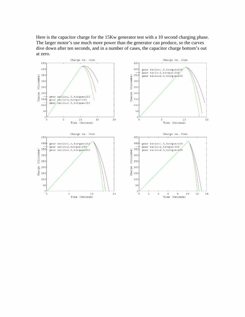
Here is the capacitor charge for the 15Kw generator test with a 10 second charging phase. The larger motor’s use much more power than the generator can produce, so the curves dive down after ten seconds, and in a number of cases, the capacitor charge bottom’s out at zero.

Here are velocity curves for 15kW generator test with a 10 second charging phase. The velocity curves for the large motors show a large decrease in slope when the capacitor run out of charge.

Here are the race results for the 15kW generator with a 10 second charging phase.

This set of test was run using a 30kW generator with a 10 second charging phase. In this case all the motor’s had the required power for the whole run.

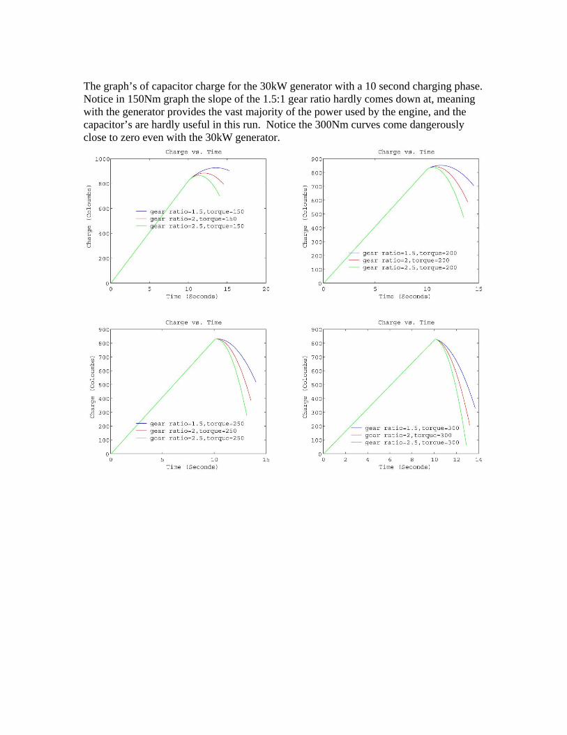
The graph’s of capacitor charge for the 30kW generator with a 10 second charging phase. Notice in 150Nm graph the slope of the 1.5:1 gear ratio hardly comes down at, meaning with the generator provides the vast majority of the power used by the engine, and the capacitor’s are hardly useful in this run. Notice the 300Nm curves come dangerously close to zero even with the 30kW generator.

The velocity curves for a ten second charging phase and a 30kW generator.

The race results for the 30kW generator with a 10 second charging phase.

To show the limitations on maximum rpm, a test was run using a 30kW generator, a 10 second charging period, and the distance covered was extended from 75m to 225m. In all cases the gear ratio of 2.5:1 maxed out the motor rpm. As the motor reaches its maximum rpm, the torque falls of to zero and the acceleration likewise goes to zero as shown in these graphs.

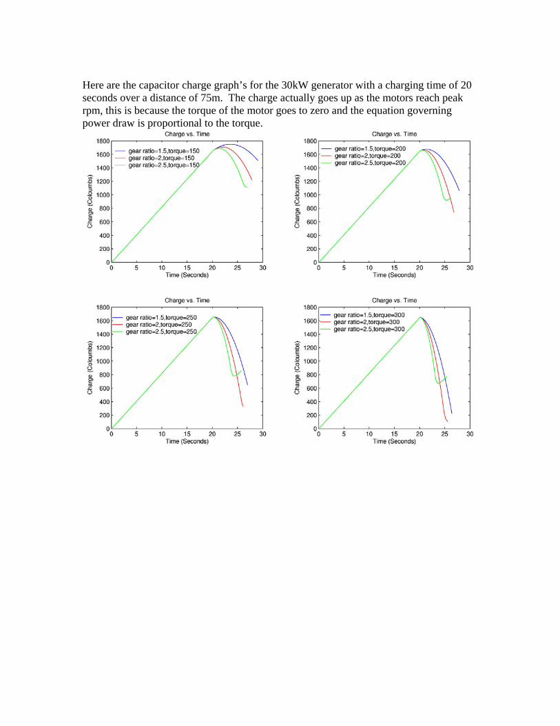
Here are the capacitor charge graph’s for the 30kW generator with a charging time of 20 seconds over a distance of 75m. The charge actually goes up as the motors reach peak rpm, this is because the torque of the motor goes to zero and the equation governing power draw is proportional to the torque.

Here are the capacitor charge graph’s for the 30kW generator with a charging time of 20 seconds over a distance of 75m. All the velocity curves tail off as the motor reaches peak rpms. For the two larger motor’s the higher gear ratio hits a plateau before the lower gear ratio’s and at the end of the run is actually going slower than the lower gear ratio. This is a large reason why we choose a gear ratio of 2:1 rather than a 2.5:1 ratio.

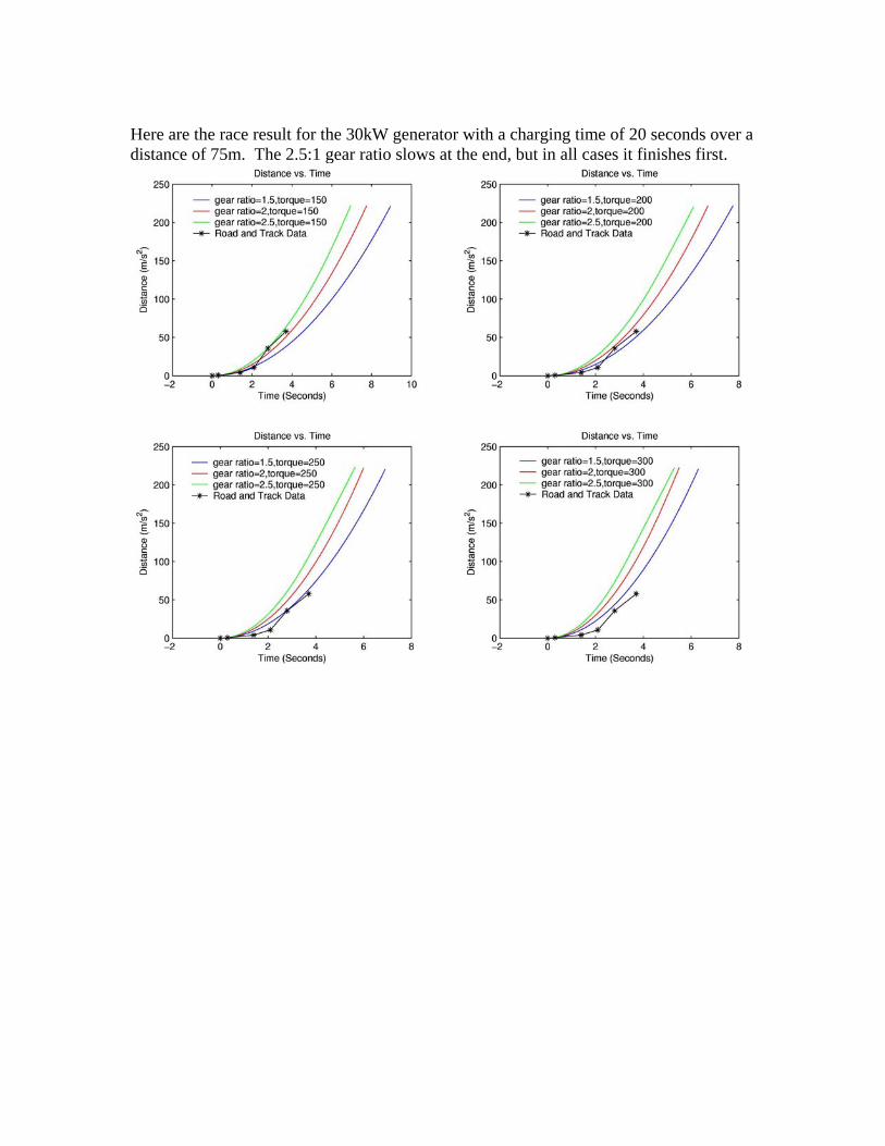
Here are the race result for the 30kW generator with a charging time of 20 seconds over a distance of 75m. The 2.5:1 gear ratio slows at the end, but in all cases it finishes first.

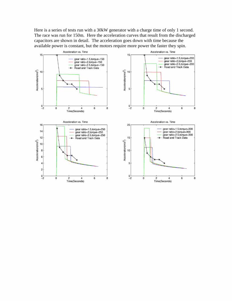
Here is a series of tests run with a 30kW generator with a charge time of only 1 second. The race was run for 150m. Here the acceleration curves that result from the discharged capacitors are shown in detail. The acceleration goes down with time because the available power is constant, but the motors require more power the faster they spin.

Here is a series of tests run with a 30kW generator with a charge time of only 1 second. The race was run for 150m. The capacitor charge is not very exciting since, they discharge quickly and stay at zero for the remainder.

Here is a series of tests run with a 30kW generator with a charge time of only 1 second. The race was run for 150m. The velocity curves level out when the capacitors discharge fully.

Here is a race results with a 30kW generator with a charge time of only 1 second. The race was run for 150m.

Appendix C

Etek Motor Specifications 20 HP Peak, 8 HP continuous Voltage........................50 VDC Max Nonload Current.....6 AMP Max Nonload Speed........3600 RPM MIN Nonload Speed.........3300 RPM Min Speed at 160 Lbln.....3200 RPM Max Current at 160 Lbln...150 AMPS Shaft Size .......................7/8" Voltage Constant: 72 RPM per volt Torque Constant: 1.14 in lbs/Amp Continuous Current: 300 A 30 Sec. Weight: 20.8 lbs Motor Diameter: 7.91" Motor Length: 5.64" Shaft Diameter: 7/8"-3/16" Keyway Price: $335 www.cloudelectric.com

http://www.motorcycle.com/mo/mccompare/01600/mcphotos/01yzfr6dyno.html

Appendix E

PC2500 Ultracapacitor Product Information

• Delivers up to 100 times the energy of conventional capacitors and delivers ten times the power of ordinary batteries

• Is optimized for individual applications through its capacity to repeatedly charge and discharge

• Offers instantaneous ride-through power

Capacitance 2700 Farads (-10%/+30%)

Series Resistance DC 1.0 mohms (-25%/+25%)

1kHz 0.55 mohms (-25%/+25%)

Voltage Continuous 2.5 V

Peak 2.7 V

Rated current1,2 625 A

Dimensions (reference only) 161 x 61.5 x 61.5 mm

Weight 725 g

Volume .6 L

Temperature3 Operating -40°C to 70°C

Storage -40°C to 85°C

Leakage Current (after 72 hours) 6 mA

Price: $50 each

Appendix F

Appendix G

Appendix H

Advanced DC L91-4003 motor

72-120 V 85 lbs

130 Amp continuous $800

13 HP continuous