ENGR 224 - Thermodynamics HW #2 Problem : 3.26 ......Baratuci HW #2 Problem : 3.26 - Steam NIST /...

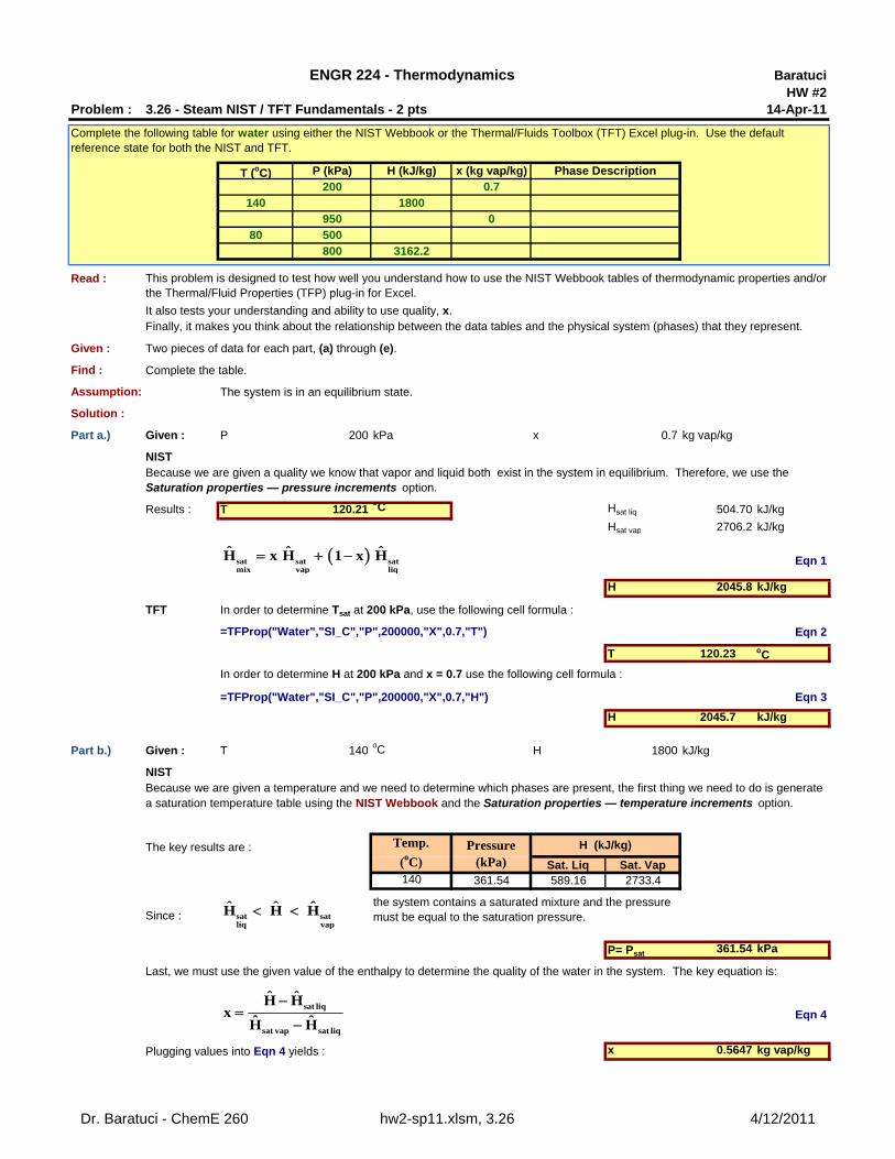
BaratuciHW #2

Problem : 3.26 - Steam NIST / TFT Fundamentals - 2 pts 14-Apr-11

T (oC) P (kPa) H (kJ/kg) x (kg vap/kg)200 0.7

140 1800950 0

80 500800 3162.2

Read :

It also tests your understanding and ability to use quality, x.

Given : Two pieces of data for each part, (a) through (e).

Find : Complete the table.

Assumption: The system is in an equilibrium state.

Solution :

Part a.) Given : P 200 kPa x 0.7 kg vap/kg

NIST

Results : T 120.21oC Hsat liq 504.70 kJ/kg

Hsat vap 2706.2 kJ/kg

Eqn 1

H 2045.8 kJ/kg

TFT In order to determine Tsat at 200 kPa, use the following cell formula :

=TFProp("Water","SI_C","P",200000,"X",0.7,"T") Eqn 2

T 120.23 oC

In order to determine H at 200 kPa and x = 0.7 use the following cell formula :

=TFProp("Water","SI_C","P",200000,"X",0.7,"H") Eqn 3

H 2045.7 kJ/kg

Part b.) Given : T 140oC H 1800 kJ/kg

NIST

The key results are :

Sat. Liq Sat. Vap140 361.54 589.16 2733.4

Since :

P= Psat 361.54 kPa

Eqn 4

Plugging values into Eqn 4 yields : x 0.5647 kg vap/kg

ENGR 224 - Thermodynamics

Complete the following table for water using either the NIST Webbook or the Thermal/Fluids Toolbox (TFT) Excel plug-in. Use the default reference state for both the NIST and TFT.

Because we are given a quality we know that vapor and liquid both exist in the system in equilibrium. Therefore, we use the Saturation properties — pressure increments option.

Because we are given a temperature and we need to determine which phases are present, the first thing we need to do is generate a saturation temperature table using the NIST Webbook and the Saturation properties — temperature increments option.

Phase Description

This problem is designed to test how well you understand how to use the NIST Webbook tables of thermodynamic properties and/or the Thermal/Fluid Properties (TFP) plug-in for Excel.

Finally, it makes you think about the relationship between the data tables and the physical system (phases) that they represent.

the system contains a saturated mixture and the pressure must be equal to the saturation pressure.

Last, we must use the given value of the enthalpy to determine the quality of the water in the system. The key equation is:

Temp.

(oC)Pressure

(kPa)H (kJ/kg)

sat sat satmix vap liq

ˆ ˆ ˆH x H 1 x H

sat satliq vap

ˆ ˆ ˆH H H

sat liq

sat vap sat liq

ˆ ˆH Hx

ˆ ˆH H

Dr. Baratuci - ChemE 260 hw2-sp11.xlsm, 3.26 4/12/2011

TFT

Hsat liq =TFProp("Water","SI_C","T",140,"X",0,"H") Eqn 5Hsat vap =TFProp("Water","SI_C","T",140,"X",1,"H") Eqn 6

Hsat liq 588.72 kJ/kgHsat vap 2733.40 kJ/kg

Since :

P =TFProp("Water","SI_C","T",140,"X",1,"P") Eqn 7

P= Psat 361.29 kPa

x =TFProp("Water","SI_C","T",140,"H",1800,"X") Eqn 7

x 0.5648 kg vap/kg

Part c.) Given : P 950 kPa x 0 kg vap/kg

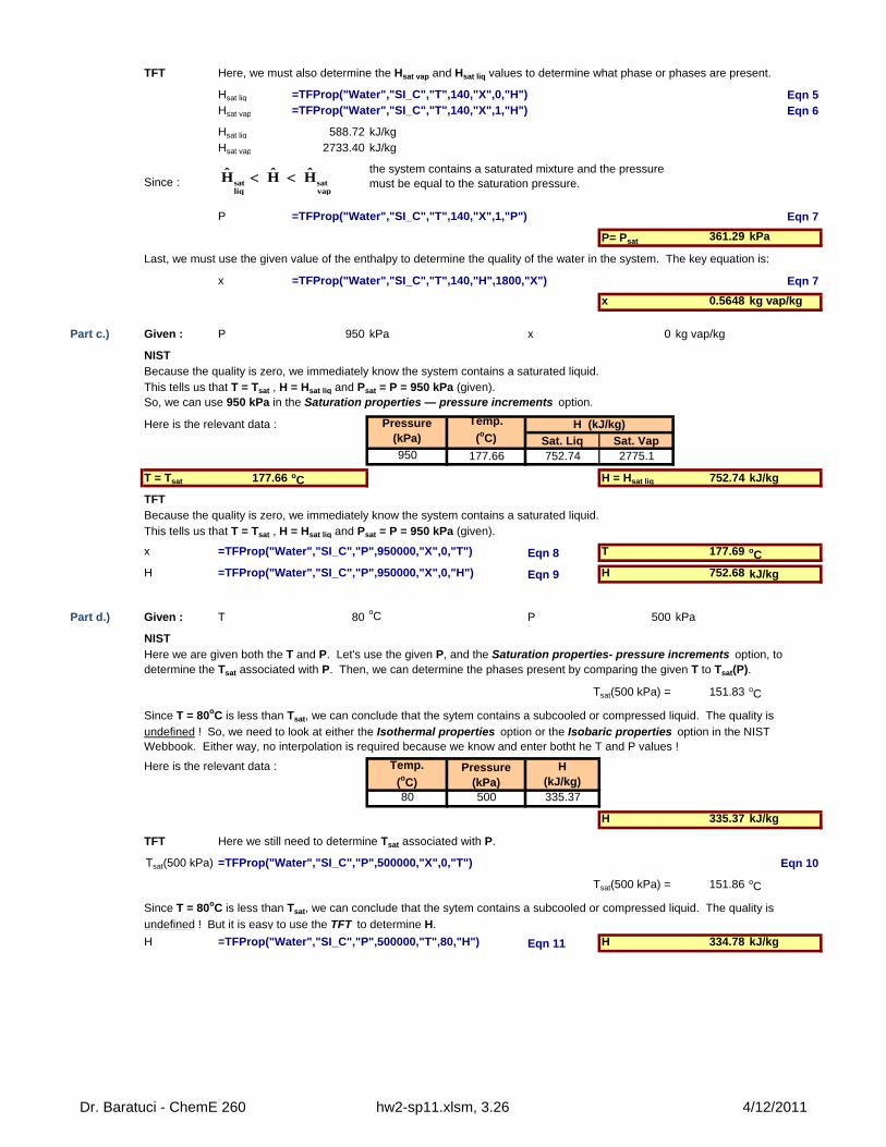
NISTBecause the quality is zero, we immediately know the system contains a saturated liquid.This tells us that T = Tsat , H = Hsat liq and Psat = P = 950 kPa (given).So, we can use 950 kPa in the Saturation properties — pressure increments option.

Here is the relevant data :

Sat. Liq Sat. Vap950 177.66 752.74 2775.1

T = Tsat 177.66 oC H = Hsat liq 752.74 kJ/kg

TFTBecause the quality is zero, we immediately know the system contains a saturated liquid.This tells us that T = Tsat , H = Hsat liq and Psat = P = 950 kPa (given).

x =TFProp("Water","SI_C","P",950000,"X",0,"T") Eqn 8 T 177.69 oC

H =TFProp("Water","SI_C","P",950000,"X",0,"H") Eqn 9 H 752.68 kJ/kg

Part d.) Given : T 80oC P 500 kPa

NIST

Tsat(500 kPa) = 151.83 oC


80 500 335.37

H 335.37 kJ/kg

TFT Here we still need to determine Tsat associated with P.

Tsat(500 kPa) =TFProp("Water","SI_C","P",500000,"X",0,"T") Eqn 10

Tsat(500 kPa) = 151.86 oC

H =TFProp("Water","SI_C","P",500000,"T",80,"H") Eqn 11 H 334.78 kJ/kg


H (kJ/kg)

Here, we must also determine the Hsat vap and Hsat liq values to determine what phase or phases are present.

the system contains a saturated mixture and the pressure must be equal to the saturation pressure.

Pressure(kPa)

Temp.

(oC)H (kJ/kg)

Here we are given both the T and P. Let's use the given P, and the Saturation properties- pressure increments option, to determine the Tsat associated with P. Then, we can determine the phases present by comparing the given T to Tsat(P).

Since T = 80oC is less than Tsat, we can conclude that the sytem contains a subcooled or compressed liquid. The quality is

undefined ! So, we need to look at either the Isothermal properties option or the Isobaric properties option in the NIST Webbook. Either way, no interpolation is required because we know and enter botht he T and P values !

Temp.

(oC)Pressure

(kPa)

Since T = 80oC is less than Tsat, we can conclude that the sytem contains a subcooled or compressed liquid. The quality is

undefined ! But it is easy to use the TFT to determine H.

sat satliq vap

ˆ ˆ ˆH H H


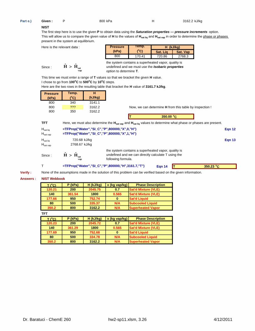
Part e.) Given : P 800 kPa H 3162.2 kJ/kg

NIST


Sat. Liq Sat. Vap800 170.41 720.86 2768.3

Since :

This time we must enter a range of T values so that we bracket the given H value.I chose to go from 100oC to 500oC by 10oC steps.Here are the two rows in the resulting table that bracket the H value of 3161.7 kJ/kg.

800 340 3141.1800 ??? 3162.2800 350 3162.2

T 350.00 oC

TFT

Hsat liq =TFProp("Water","SI_C","P",800000,"X",0,"H") Eqn 12Hsat vap =TFProp("Water","SI_C","P",800000,"X",1,"H")

Hsat liq 720.68 kJ/kg Eqn 13Hsat vap 2768.67 kJ/kg

Since :

T =TFProp("Water","SI_C","P",800000,"H",3161.7,"T") Eqn 14 T 350.23 oC

Verify :

Answers : NIST Webbook

T (oC) P (kPa) H (kJ/kg) x (kg vap/kg)120.21 200 2045.75 0.7

140 361.54 1800 0.565177.66 950 752.74 0

80 500 335.37 N/A350.2 800 3162.2 N/A

TFT

T (oC) P (kPa) H (kJ/kg) x (kg vap/kg)120.23 200 2045.72 0.7

140 361.29 1800 0.565177.69 950 752.68 0

80 500 334.78 N/A350.2 800 3162.2 N/A

Pressure(kPa)

Temp.

(oC)H (kJ/kg)

the system contains a superheated vapor, quality is undefined and we must use the Isobaric properties option to determine T.

The first step here is to use the given P to obtain data using the Saturation properties — pressure increments option.This will allow us to compare the given value of H to the values of Hsat liq and Hsat vap in order to determine the phase or phases present in the system at equilibrium.

None of the assumptions made in the solution of this problem can be verified based on the given information.

Phase DescriptionSat'd Mixture (VLE)Sat'd Mixture (VLE)Sat'd Liquid

the system contains a superheated vapor, quality is undefined and we can directly calculate T using the following formula.

Pressure(kPa)

Temp.

(oC)

Now, we can determine H from this table by inspection !


H (kJ/kg)

Subcooled Liquid

Sat'd LiquidSubcooled LiquidSuperheated Vapor

Superheated Vapor

Phase DescriptionSat'd Mixture (VLE)Sat'd Mixture (VLE)

satvap

ˆ ˆH H

satvap

ˆ ˆH H


BaratuciHW #2

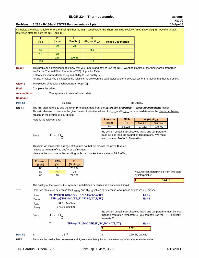
Problem : 3.29E - R-134a NIST/TFT Fundamentals - 2 pts 14-Apr-11

T

(oF)

P(psia)

H(Btu/lbm)

x(lbm vap/lbm)

80 78

15 0.6

10 70180 129.46

110 1.0

Read :

It also tests your understanding and ability to use quality, x.

Given : Two pieces of data for each part, (a) through (e).

Find : Complete the table.

Assumptions: The system is in an equilibrium state.

Solution :

Part a.) P 80 psia H 78 Btu/lbm

NIST :


Sat. Liq Sat. Vap80 65.922 97.162 176.02

Since :

This time we must enter a range of T values so that we bracket the given H value.I chose to go from 0oF to 100oF by 10oF steps.

Here are the two rows in the resulting table that bracket the H value of 78 Btu/lbm .

80 0 75.99480 ??? 7880 10 79.107

T 6.44oF

TFT :

Hsat liq =TFProp("R-134a","EE_F","P",80,"X",0,"H") Eqn 2Hsat vap =TFProp("R-134a","EE_F","P",80,"X",1,"H") Eqn 3

Hsat liq 97.11 Btu/lbmHsat vap 175.90 Btu/lbm

Since :

T =TFProp("R-134a","EE_F","P",80,"H",78,"T") Eqn 4

T 6.62oF

Part b.) T 15oF x 0.60 lbm vap/lbm

NIST :

Now, we can determine T from this table by interpolation.

The quality of the water in the system is not defined because it is a subcooled liquid.


Complete the following table for R-134a using either the NIST Webbook or the Thermal/Fluids Toolbox (TFT) Excel plug-in. Use the default reference state for both the NIST and TFT.

Phase Description

This problem is designed to test how well you understand how to use the NIST Webbook tables of thermodynamic properties and/or the Thermal/Fluid Properties (TFP) plug-in for Excel.

Finally, it makes you think about the relationship between the data tables and the physical system (phases) that they represent.

Pressure(psia)

Temp.

(oF)

H (Btu/lbm)

The first step here is to use the given P to obtain data from the Saturation properties — pressure increments option.


the system contains a subcooled liquid and temperature must be less than the saturation temperature. We can now use the TFT to directly evaluate T.

Because the quality lies between 0 and 1, we immediately know the system contains a saturated mixture.

This will allow us to compare the given value of H to the values of Hsat liq and Hsat vap in order to determine the phase or phases present in the system at equilibrium.

Pressure(psia)

Temp.

(oF)H (Btu/lbm)

the system contains a subcooled liquid and temperature must be less than the saturation temperature. We must interpolate on Isobaric Properties .

satliq

ˆ ˆH H

satliq

ˆ ˆH H

Dr. Baratuci - ChemE 260 hw2-sp11.xlsm, 3.29E 4/12/2011

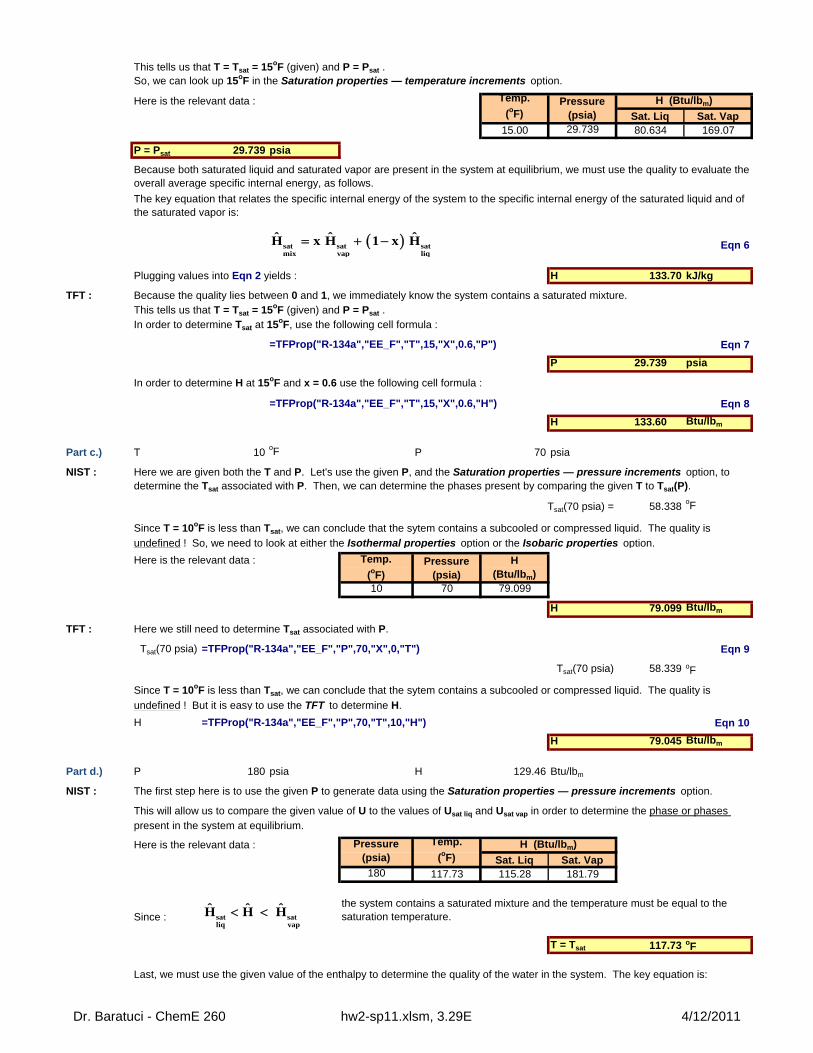
This tells us that T = Tsat = 15oF (given) and P = Psat .So, we can look up 15oF in the Saturation properties — temperature increments option.


Sat. Liq Sat. Vap15.00 29.739 80.634 169.07

P = Psat 29.739 psia

Eqn 6

Plugging values into Eqn 2 yields : H 133.70 kJ/kg

TFT :This tells us that T = Tsat = 15oF (given) and P = Psat .In order to determine Tsat at 15oF, use the following cell formula :

=TFProp("R-134a","EE_F","T",15,"X",0.6,"P") Eqn 7

P 29.739 psia

In order to determine H at 15oF and x = 0.6 use the following cell formula :

=TFProp("R-134a","EE_F","T",15,"X",0.6,"H") Eqn 8

H 133.60 Btu/lbm

Part c.) T 10oF P 70 psia

NIST :

Tsat(70 psia) = 58.338oF


10 70 79.099

H 79.099 Btu/lbm

TFT : Here we still need to determine Tsat associated with P.

Tsat(70 psia) =TFProp("R-134a","EE_F","P",70,"X",0,"T") Eqn 9

Tsat(70 psia) 58.339 oF

H =TFProp("R-134a","EE_F","P",70,"T",10,"H") Eqn 10

H 79.045 Btu/lbm

Part d.) P 180 psia H 129.46 Btu/lbm

NIST :


Sat. Liq Sat. Vap180 117.73 115.28 181.79

Since :

T = Tsat 117.73 oF

Pressure(psia)

H (Btu/lbm)

Here we are given both the T and P. Let's use the given P, and the Saturation properties — pressure increments option, to determine the Tsat associated with P. Then, we can determine the phases present by comparing the given T to Tsat(P).

Since T = 10oF is less than Tsat, we can conclude that the sytem contains a subcooled or compressed liquid. The quality is

undefined ! So, we need to look at either the Isothermal properties option or the Isobaric properties option.

The key equation that relates the specific internal energy of the system to the specific internal energy of the saturated liquid and of the saturated vapor is:

Because the quality lies between 0 and 1, we immediately know the system contains a saturated mixture.

Pressure(psia)

Temp.

(oF)H (Btu/lbm)

Temp.

(oF)

Because both saturated liquid and saturated vapor are present in the system at equilibrium, we must use the quality to evaluate the overall average specific internal energy, as follows.

Temp.

(oF)Pressure

(psia)H (Btu/lbm)

Since T = 10oF is less than Tsat, we can conclude that the sytem contains a subcooled or compressed liquid. The quality is

undefined ! But it is easy to use the TFT to determine H.

The first step here is to use the given P to generate data using the Saturation properties — pressure increments option.

This will allow us to compare the given value of U to the values of Usat liq and Usat vap in order to determine the phase or phases present in the system at equilibrium.

the system contains a saturated mixture and the temperature must be equal to the saturation temperature.



ˆ ˆ ˆH x H 1 x H

sat satliq vap

ˆ ˆ ˆH H H


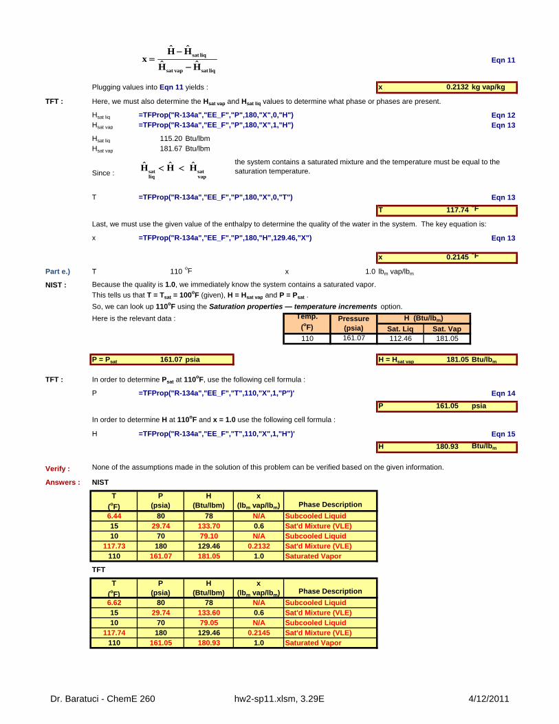
Eqn 11

Plugging values into Eqn 11 yields : x 0.2132 kg vap/kg

TFT :

Hsat liq =TFProp("R-134a","EE_F","P",180,"X",0,"H") Eqn 12Hsat vap =TFProp("R-134a","EE_F","P",180,"X",1,"H") Eqn 13

Hsat liq 115.20 Btu/lbmHsat vap 181.67 Btu/lbm

Since :

T =TFProp("R-134a","EE_F","P",180,"X",0,"T") Eqn 13

T 117.74oF

x =TFProp("R-134a","EE_F","P",180,"H",129.46,"X") Eqn 13

x 0.2145oF

Part e.) T 110oF x 1.0 lbm vap/lbm

NIST : Because the quality is 1.0, we immediately know the system contains a saturated vapor.

This tells us that T = Tsat = 100oF (given), H = Hsat vap and P = Psat .


Sat. Liq Sat. Vap110 161.07 112.46 181.05

P = Psat 161.07 psia H = Hsat vap 181.05 Btu/lbm

TFT : In order to determine Psat at 110oF, use the following cell formula :

P =TFProp("R-134a","EE_F","T",110,"X",1,"P")' Eqn 14

P 161.05 psia

In order to determine H at 110oF and x = 1.0 use the following cell formula :

H =TFProp("R-134a","EE_F","T",110,"X",1,"H")' Eqn 15

H 180.93 Btu/lbm

Verify :

Answers : NIST

T

(oF)

P(psia)

H(Btu/lbm)

x(lbm vap/lbm)

6.44 80 78 N/A15 29.74 133.70 0.610 70 79.10 N/A

117.73 180 129.46 0.2132110 161.07 181.05 1.0

TFT

T

(oF)

P(psia)

H(Btu/lbm)

x(lbm vap/lbm)

6.62 80 78 N/A15 29.74 133.60 0.610 70 79.05 N/A

117.74 180 129.46 0.2145110 161.05 180.93 1.0

So, we can look up 110oF using the Saturation properties — temperature increments option.

Pressure(psia)

H (Btu/lbm)




Saturated Vapor

Subcooled LiquidSat'd Mixture (VLE)Saturated Vapor

Phase Description

Sat'd Mixture (VLE)Subcooled LiquidSat'd Mixture (VLE)

Subcooled LiquidSat'd Mixture (VLE)

Phase Description

Subcooled Liquid


Temp.

(oF)

sat liq

sat vap sat liq

ˆ ˆH Hx

ˆ ˆH H

sat satliq vap

ˆ ˆ ˆH H H


BaratuciHW #2

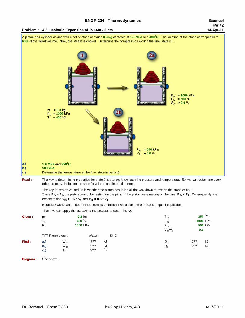
Problem : 4.8 - Isobaric Expansion of R-134a - 6 pts 14-Apr-11

a.) 1.0 MPa and 250oCb.) 500 kPac.) Determine the temperature at the final state in part (b)

Read :

The key for states 2a and 2b is whether the piston has fallen all the way down to rest on the stops or not.

Then, we can apply the 1st Law to the process to determine Q.

Given : m 0.3 kg T2a 250oC

T1 400oC P2a 1000 kPa

P1 1000 kPa P2b 500 kPaV2b/V1 0.6

TFT Parameters : Water SI_C

Find : a.) Wba ??? kJ Qa ??? kJb.) Wbb ??? kJ Qb ??? kJc.) T2b ???

oC

Diagram : See above.

Since P2a = P1, the piston cannot be resting on the pins. If the piston were resting on the pins, P2a < P1. Consequently, we

expect to find V2a > 0.6 * V1 and V2b = 0.6 * V1.

A piston-and-cylinder device with a set of stops contains 0.3 kg of steam at 1.0 MPa and 400oC. The location of the stops corresponds to 60% of the initial volume. Now, the steam is cooled. Determine the compression work if the final state is…

The key to determining properties for state 1 is that we know both the pressure and temperature. So, we can determine every other property, including the specific volume and internal energy.


Boundary work can be determined from its definition if we assume the process is quasi-equilibrium.

m = 0.3 kgP1 = 1000 kPaT1 = 400 oC

P2a = 1000 kPaT2a = 250 oCV2a > 0.6 V1

P2b = 500 kPaV2b = 0.6 V1


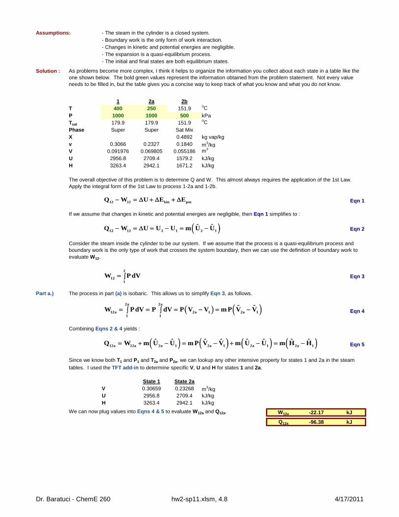
Assumptions: - The steam in the cylinder is a closed system.- Boundary work is the only form of work interaction.- Changes in kinetic and potential energies are negligible.- The expansion is a quasi-equilibrium process.- The initial and final states are both equilibrium states.

Solution :

1 2a 2bT 400 250 151.9

oC

P 1000 1000 500 kPaTsat 179.9 179.9 151.9

oC

Phase Super Super Sat MixX 0.4892 kg vap/kgv 0.3066 0.2327 0.1840 m3/kgV 0.091976 0.069805 0.055186 m3

U 2956.8 2709.4 1579.2 kJ/kgH 3263.4 2942.1 1671.2 kJ/kg

Eqn 1

Eqn 2

Eqn 3

Part a.)

Eqn 4

Eqn 5

State 1 State 2aV 0.30659 0.23268 m3/kgU 2956.8 2709.4 kJ/kgH 3263.4 2942.1 kJ/kg

We can now plug values into Eqns 4 & 5 to evaluate W12a and Q12a. W12a -22.17 kJ

Q12a -96.38 kJ

Combining Eqns 2 & 4 yields :

Since we know both T1 and P1 and T2a and P2a, we can lookup any other intensive property for states 1 and 2a in the steam

tables. I used the TFT add-in to determine specific V, U and H for states 1 and 2a.

If we assume that changes in kinetic and potential energies are negligible, then Eqn 1 simplifies to :

Consider the steam inside the cylinder to be our system. If we assume that the process is a quasi-equilibrium process and boundary work is the only type of work that crosses the system boundary, then we can use the definition of boundary work to evaluate W12.

The process in part (a) is isobaric. This allows us to simplify Eqn 3, as follows.

As problems become more complex, I think it helps to organize the information you collect about each state in a table like the one shown below. The bold green values represent the information obtained from the problem statement. Not every value needs to be filled in, but the table gives you a concise way to keep track of what you know and what you do not know.

The overall objective of this problem is to determine Q and W. This almost always requires the application of the 1st Law. Apply the integral form of the 1st Law to process 1-2a and 1-2b.

12 12 kin potQ W U E E

12 12 2 1 2 1ˆ ˆQ W U U U m U U

2

121

W PdV

2a 2a

12a 2a 1 2a 11 1

ˆ ˆW PdV P dV P V V m P V V

12a 12a 2a 1 2a 1 2a 1 2a 1ˆ ˆ ˆ ˆ ˆ ˆ ˆ ˆQ W m U U m P V V m U U m H H


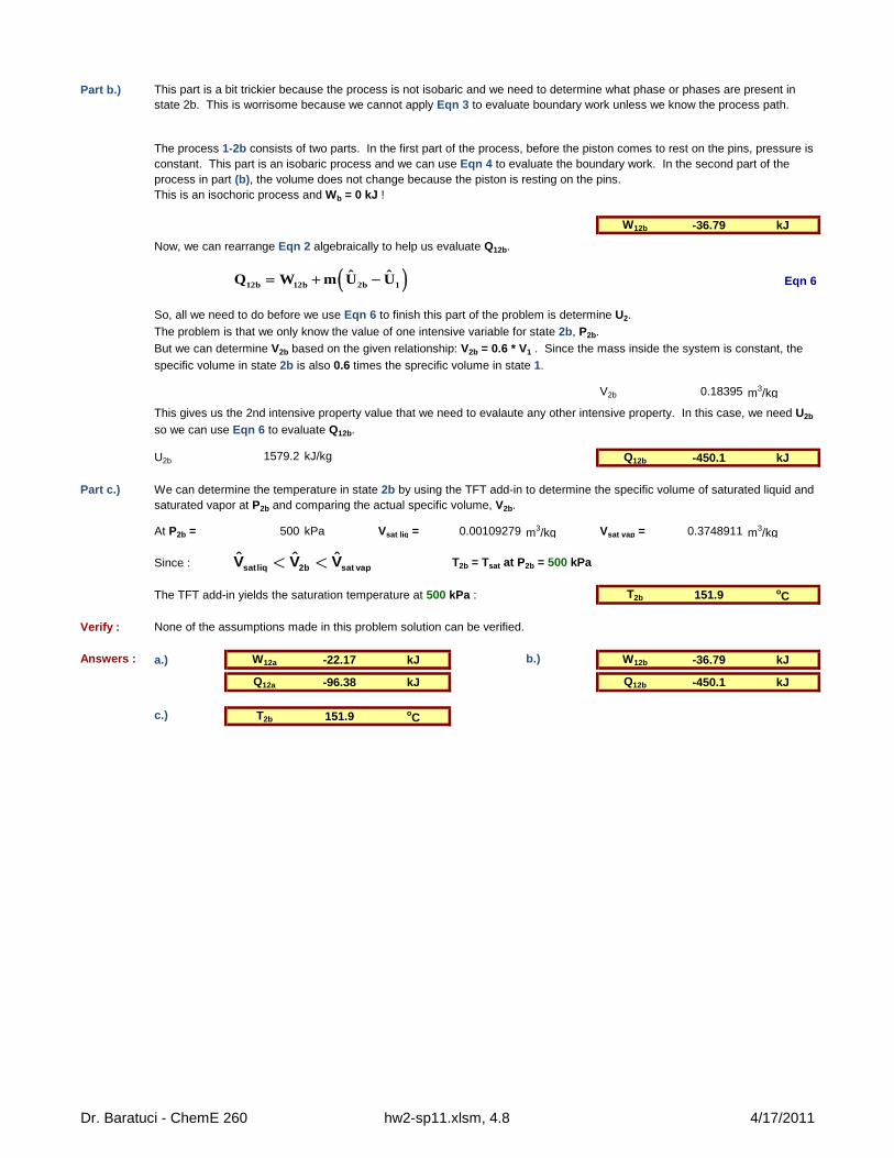
Part b.)

W12b -36.79 kJ

Now, we can rearrange Eqn 2 algebraically to help us evaluate Q12b.

Eqn 6

V2b 0.18395 m3/kg

U2b 1579.2 kJ/kg Q12b -450.1 kJ

Part c.)

At P2b = 500 kPa Vsat liq = 0.00109279 m3/kg Vsat vap = 0.3748911 m3/kg

Since : T2b = Tsat at P2b = 500 kPa

The TFT add-in yields the saturation temperature at 500 kPa : T2b 151.9 oC

Verify : None of the assumptions made in this problem solution can be verified.

Answers : a.) W12a -22.17 kJ b.) W12b -36.79 kJ

Q12a -96.38 kJ Q12b -450.1 kJ

c.) T2b 151.9 oC

We can determine the temperature in state 2b by using the TFT add-in to determine the specific volume of saturated liquid and saturated vapor at P2b and comparing the actual specific volume, V2b.

This part is a bit trickier because the process is not isobaric and we need to determine what phase or phases are present in state 2b. This is worrisome because we cannot apply Eqn 3 to evaluate boundary work unless we know the process path.

The process 1-2b consists of two parts. In the first part of the process, before the piston comes to rest on the pins, pressure is constant. This part is an isobaric process and we can use Eqn 4 to evaluate the boundary work. In the second part of the process in part (b), the volume does not change because the piston is resting on the pins.This is an isochoric process and Wb = 0 kJ !

So, all we need to do before we use Eqn 6 to finish this part of the problem is determine U2.

The problem is that we only know the value of one intensive variable for state 2b, P2b.

But we can determine V2b based on the given relationship: V2b = 0.6 * V1 . Since the mass inside the system is constant, the

specific volume in state 2b is also 0.6 times the sprecific volume in state 1.

This gives us the 2nd intensive property value that we need to evalaute any other intensive property. In this case, we need U2b

so we can use Eqn 6 to evaluate Q12b.

12b 12b 2b 1ˆ ˆQ W m U U

satliq 2b sat vapˆ ˆ ˆV V V< <


BaratuciHW #2

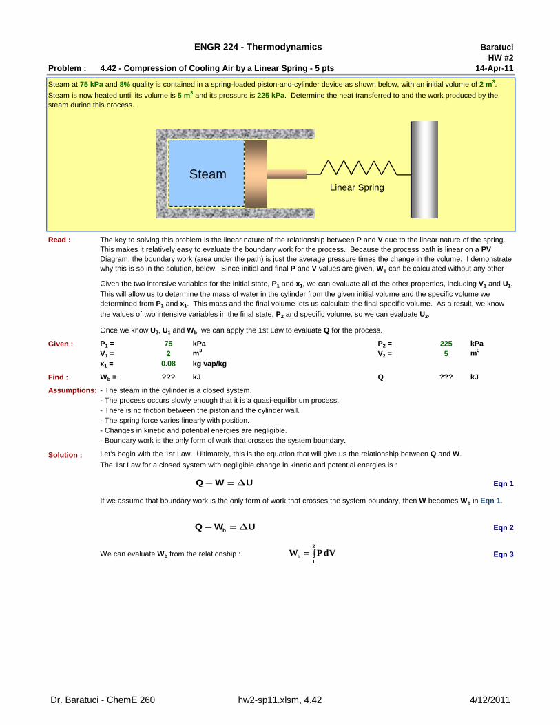
Problem : 4.42 - Compression of Cooling Air by a Linear Spring - 5 pts 14-Apr-11

Read :

Given : P1 = 75 kPa P2 = 225 kPaV1 = 2 m3 V2 = 5 m3

x1 = 0.08 kg vap/kg

Find : Wb = ??? kJ Q ??? kJ

Assumptions: - The steam in the cylinder is a closed system.- The process occurs slowly enough that it is a quasi-equilibrium process.- There is no friction between the piston and the cylinder wall.- The spring force varies linearly with position.- Changes in kinetic and potential energies are negligible.- Boundary work is the only form of work that crosses the system boundary.

Solution :

Eqn 1

Eqn 2

We can evaluate Wb from the relationship : Eqn 3

Let's begin with the 1st Law. Ultimately, this is the equation that will give us the relationship between Q and W.

If we assume that boundary work is the only form of work that crosses the system boundary, then W becomes Wb in Eqn 1.


Steam at 75 kPa and 8% quality is contained in a spring-loaded piston-and-cylinder device as shown below, with an initial volume of 2 m3.

Steam is now heated until its volume is 5 m3 and its pressure is 225 kPa. Determine the heat transferred to and the work produced by the steam during this process.

The key to solving this problem is the linear nature of the relationship between P and V due to the linear nature of the spring. This makes it relatively easy to evaluate the boundary work for the process. Because the process path is linear on a PV Diagram, the boundary work (area under the path) is just the average pressure times the change in the volume. I demonstrate why this is so in the solution, below. Since initial and final P and V values are given, Wb can be calculated without any other

Given the two intensive variables for the initial state, P1 and x1, we can evaluate all of the other properties, including V1 and U1.

This will allow us to determine the mass of water in the cylinder from the given initial volume and the specific volume we determined from P1 and x1. This mass and the final volume lets us calculate the final specific volume. As a result, we know

the values of two intensive variables in the final state, P2 and specific volume, so we can evaluate U2.

Once we know U2, U1 and Wb, we can apply the 1st Law to evaluate Q for the process.

The 1st Law for a closed system with negligible change in kinetic and potential energies is :

SteamLinear Spring

Q W U- = D

bQ W U- =D

2

b1

W PdV


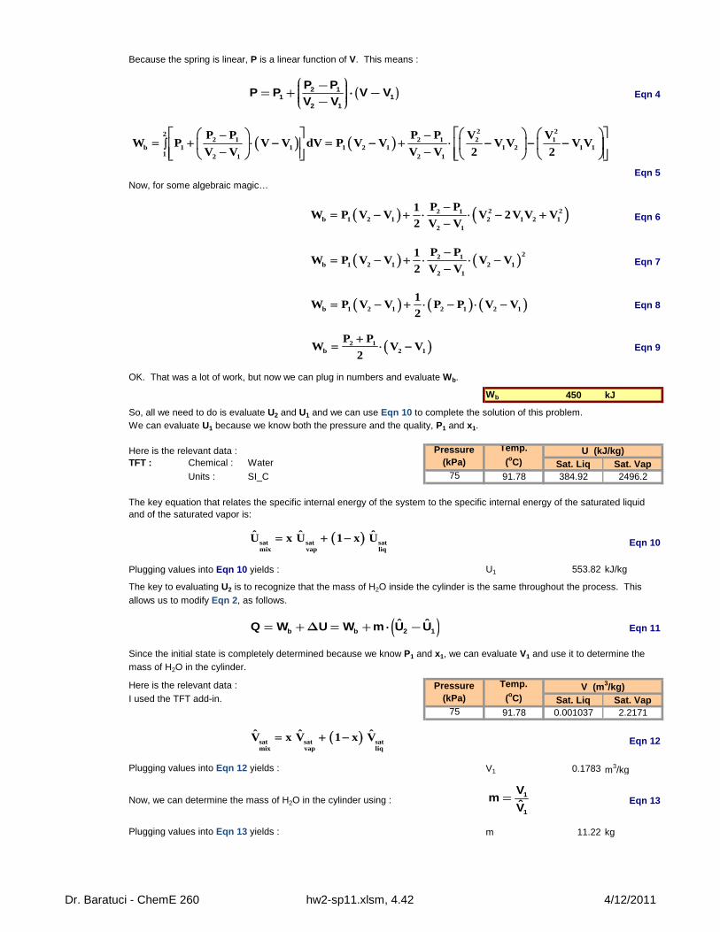
Eqn 4

Eqn 5Now, for some algebraic magic…

Eqn 6

Eqn 7

Eqn 8

Eqn 9

OK. That was a lot of work, but now we can plug in numbers and evaluate Wb.

Wb 450 kJ

So, all we need to do is evaluate U2 and U1 and we can use Eqn 10 to complete the solution of this problem.

Here is the relevant data :TFT : Chemical : Water Sat. Liq Sat. Vap

Units : SI_C 75 91.78 384.92 2496.2

Eqn 10

Plugging values into Eqn 10 yields : U1 553.82 kJ/kg

Eqn 11


I used the TFT add-in. Sat. Liq Sat. Vap75 91.78 0.001037 2.2171

Eqn 12

Plugging values into Eqn 12 yields : V1 0.1783 m3/kg

Now, we can determine the mass of H2O in the cylinder using : Eqn 13

Plugging values into Eqn 13 yields : m 11.22 kg

Since the initial state is completely determined because we know P1 and x1, we can evaluate V1 and use it to determine the

mass of H2O in the cylinder.

Pressure(kPa)

Temp.

(oC)V (m3/kg)

The key to evaluating U2 is to recognize that the mass of H2O inside the cylinder is the same throughout the process. This

allows us to modify Eqn 2, as follows.

We can evaluate U1 because we know both the pressure and the quality, P1 and x1.

Pressure(kPa)

Temp.

(oC)U (kJ/kg)

The key equation that relates the specific internal energy of the system to the specific internal energy of the saturated liquid and of the saturated vapor is:

Because the spring is linear, P is a linear function of V. This means :

2 22

2 1 2 1 2 1b 1 1 1 2 1 1 2 1 1

1 2 1 2 1

P P P P V VW P V V dV P V V V V V V

V V V V 2 2

( )2 11 1

2 1

P PP P V V

V V

æ ö-ç ÷= + ⋅ -ç ÷ç ÷ç ÷-è ø

2 22 1b 1 2 1 2 1 2 1

2 1

P P1W P V V V 2V V V

2 V V

22 1b 1 2 1 2 1

2 1

P P1W P V V V V

2 V V

b 1 2 1 2 1 2 1

1W P V V P P V V

2

2 1b 2 1

P PW V V

2


ˆ ˆ ˆU x U 1 x U


ˆ ˆ ˆV x V 1 x V

1

1

Vm

V=

( )b b 2 1ˆ ˆQ W U W m U U= +D = + ⋅ -


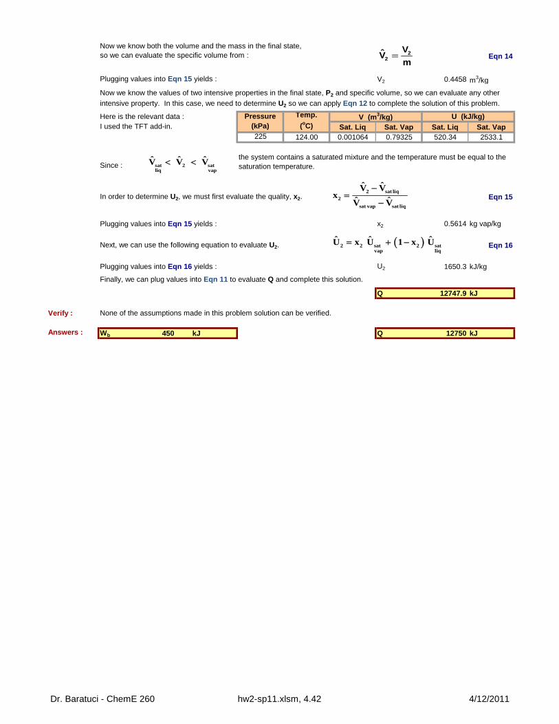
Eqn 14

Plugging values into Eqn 15 yields : V2 0.4458 m3/kg

Here is the relevant data :I used the TFT add-in. Sat. Liq Sat. Vap Sat. Liq Sat. Vap

225 124.00 0.001064 0.79325 520.34 2533.1

Since :

In order to determine U2, we must first evaluate the quality, x2. Eqn 15

Plugging values into Eqn 15 yields : x2 0.5614 kg vap/kg

Next, we can use the following equation to evaluate U2. Eqn 16

Plugging values into Eqn 16 yields : U2 1650.3 kJ/kg

Finally, we can plug values into Eqn 11 to evaluate Q and complete this solution.

Q 12747.9 kJ


Answers : Wb 450 kJ Q 12750 kJ


U (kJ/kg)

Now we know both the volume and the mass in the final state,so we can evaluate the specific volume from :

Now we know the values of two intensive properties in the final state, P2 and specific volume, so we can evaluate any other

intensive property. In this case, we need to determine U2 so we can apply Eqn 12 to complete the solution of this problem.

Pressure(kPa)

Temp.

(oC)V (m3/kg)

22

VV

m=

sat 2 satliq vap

ˆ ˆ ˆV V V

2 sat liq

2

sat vap sat liq

ˆ ˆV Vx

ˆ ˆV V

2 2 sat 2 satvap liq

ˆ ˆ ˆU x U 1 x U


BaratuciHW #2

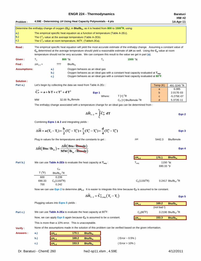
Problem : 4.59E - Determining H Using Heat Capacity Polynomials - 4 pts 14-Apr-11

a.) The empirical specific heat equation as a function of temperature (Table A-2Ec).b.)c.)

Read :

Given : T1 800 oR T2 1500 oR

Find : H1-2 = ??? Btu/lbm

Assumptions: a.) Oxygen behaves as an ideal gasb.) Oxygen behaves as an ideal gas with a constant heat capacity evaluated at Tavg.c.) Oxygen behaves as an ideal gas with a constant heat capacity evaluated at 80oF.

Solution :

Part a.) Let's begin by collecting the data we need from Table A-2Ec : Temp (K) 491-3240 oRa 6.085

Eqn 1 b 2.017E-03Where: T [=] oR c -5.275E-07

MW 32.00 lbm/lbmole CP [=] Btu/lbmole-oR d 5.372E-11

The enthalpy change associated with a temperature change for an ideal gas can be determined from :

Eqn 2

Combining Eqns 1 & 2 and integrating yields :

Eqn 3

Plug in values for the temperatures and the constants to get : H 5442.3 Btu/lbmole

Eqn 4

H1-2 170.1 Btu/lbm

Part b.) We can use Table A-2Eb to evaluate the heat capacity at Tavg : Tavg 1150 oR690.33 oF

T (oF)

CP

Btu/lbm-oR

600 0.239690.33 Cp(1150oR) Cp(1150oR) 0.2417 Btu/lbm-oR

700 0.242

Now we can use Eqn 2 to determine H1-2. It is easier to integrate this time because CP is assumed to be constant.

Eqn 5

Plugging values into Eqns 5 yields : H1-2 169.2 Btu/lbm

(not bad !)

Part c.) We can use Table A-2Ea to evaluate the heat capacity at 80oF: Cp(80oF) 0.2190 Btu/lbm-oR

Now, we can apply Eqn 5 again because CP is assumed to be a constant. H1-2 153.3 Btu/lbm

This is more than a 10% error. This is unacceptable.

Verify :

Answers : a.) H1-2 170.1 Btu/lbm

b.) H1-2 169.2 Btu/lbm ( Error ~ 0.5% )

c.) H1-2 153.3 Btu/lbm ( Error > 10% )



Determine the enthalpy change of oxygen (O2), in Btu/lbm, as it is heated from 800 to 1500oR, using:

The empirical specific heat equation will yield the most accurate estimate of the enthalpy change. Assuming a constant value of Cp determined at the average temperature should yield a reasonable estimate of H as well. Using the Cp value at room

temperature should not be very accurate. We can compare this result to the value we get in part (a).

The CoP value at the average temperature (Table A-2Eb).

The CoP value at room temperature, 80oF, (TableA-2Ea).

2

1

To

1 2 PT

H C dT

o 2 3PC a b T cT d T

m

m

H Btu / lbmoleH Btu / lb

MW lb / lbmole

2 2 3 3 4 42 1 2 1 2 1 2 1

b c dH a(T T ) (T T ) (T T ) (T T )

2 3 4

o1 2 P,avg 2 1

ˆH C T T

Dr. Baratuci - ChemE 260 hw2-sp11.xlsm , 4.59E 4/12/2011

BaratuciHW #2

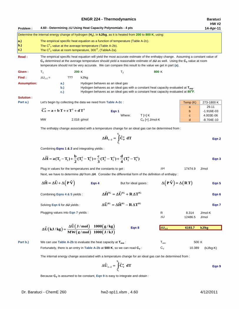
Problem : 4.60 - Determining U Using Heat Capacity Polynomials - 4 pts 14-Apr-11

a.) The empirical specific heat equation as a function of temperature (Table A-2c).b.)c.)

Read :

Given : T1 200 K T2 800 K

Find : U1-2 = ??? kJ/kg

Assumption: a.) Hydogen behaves as an ideal gasb.) Hydogen behaves as an ideal gas with a constant heat capacity evaluated at Tavg.c.) Hydogen behaves as an ideal gas with a constant heat capacity evaluated at 80oF.

Solution :

Part a.) Let's begin by collecting the data we need from Table A-2c : Temp (K) 273-1800 K

a 29.11Eqn 1 b -1.916E-03

Where: T [=] K c 4.003E-06MW 2.016 g/mol CP [=] J/mol-K d -8.704E-10

The enthalpy change associated with a temperature change for an ideal gas can be determined from :

Eqn 2

Combining Eqns 1 & 2 and integrating yields :

Eqn 3

Plug in values for the temperatures and the constants to get : H 17474.9 J/mol

Next, we have to determine U from H. Consider the differential form of the definition of enthalpy :

Eqn 4 But for ideal gases : Eqn 5

Combining Eqns 4 & 5 yields : Eqn 6

Solving Eqn 6 for U yields : Eqn 7

Plugging values into Eqn 7 yields : R 8.314 J/mol-KU 12486.5 J/mol

Eqn 8 U1-2 6193.7 kJ/kg

Part b.) We can use Table A-2b to evaluate the heat capacity at Tavg : Tavg 500 K

Fortunately, there is an entry in Table A-2b at 500 K, so we can read CV : CV 10.389 (kJ/kg-K)

The internal energy change associated with a temperature change for an ideal gas can be determined from :

Eqn 9

Because CV is assumed to be constant, Eqn 9 is easy to integrate and obtain :


Determine the internal energy change of hydrogen (H2), in kJ/kg, as it is heated from 200 to 800 K, using:

The empirical specific heat equation will yield the most accurate estimate of the enthalpy change. Assuming a constant value of CV determined at the average temperature should yield a reasonable estimate of U as well. Using the CV value at room

temperature should not be very accurate. We can compare this result to the value we get in part (a).

The CoV value at the average temperature (Table A-2b).

The CoV value at room temperature, 300 K, (TableA-2a).

U J / mol 1000 g / kgU kJ / kg

MW g / mol 1000 J / kJ

H U P V

IG IG IGH U R T

IG IG IGU H R T

2

1

To

1 2 PT

H C dT

o 2 3PC a b T cT d T

2 2 3 3 4 42 1 2 1 2 1 2 1

b c dH a(T T ) (T T ) (T T ) (T T )

2 3 4

P V R T

2

1

To

1 2 VT

ˆU C dT

Dr. Baratuci - ChemE 260 hw2-sp11.xlsm , 4.60 4/12/2011

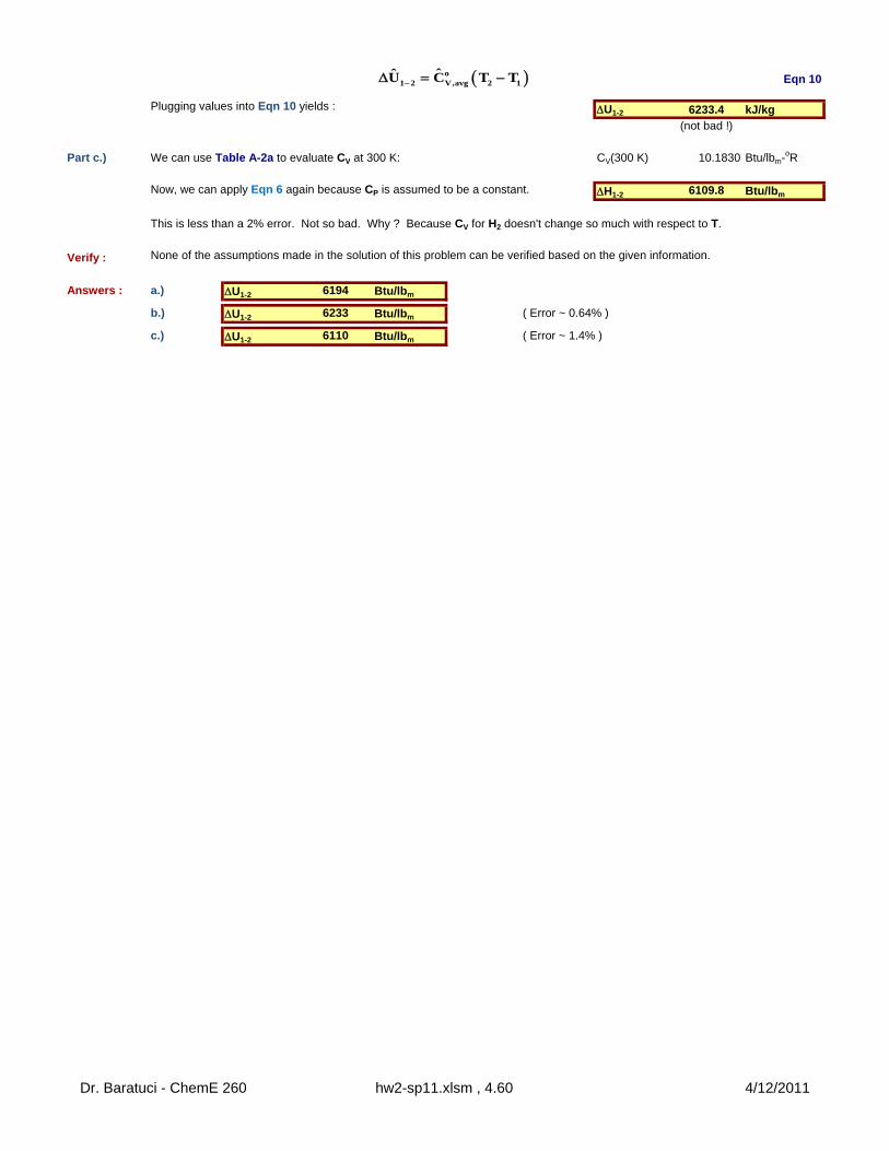
Eqn 10

Plugging values into Eqn 10 yields : U1-2 6233.4 kJ/kg(not bad !)

Part c.) We can use Table A-2a to evaluate CV at 300 K: CV(300 K) 10.1830 Btu/lbm-oR

Now, we can apply Eqn 6 again because CP is assumed to be a constant. H1-2 6109.8 Btu/lbm

This is less than a 2% error. Not so bad. Why ? Because CV for H2 doesn't change so much with respect to T.

Verify :

Answers : a.) U1-2 6194 Btu/lbm

b.) U1-2 6233 Btu/lbm ( Error ~ 0.64% )

c.) U1-2 6110 Btu/lbm ( Error ~ 1.4% )


o1 2 V,avg 2 1

ˆU C T T

Dr. Baratuci - ChemE 260 hw2-sp11.xlsm , 4.60 4/12/2011

BaratuciHW #2

Problem : WB-1 - Clapeyron & Clausius-Clapeyron Equations - 5 pts 14-Apr-11

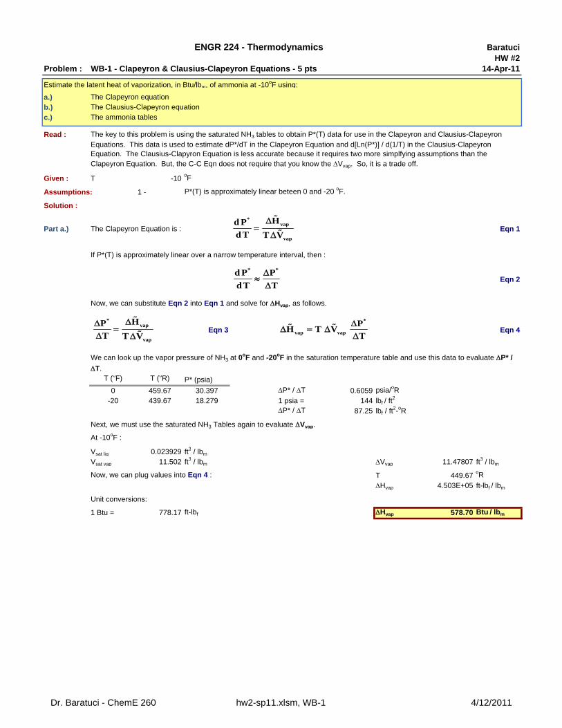
Estimate the latent heat of vaporization, in Btu/lbm, of ammonia at -10oF using:

a.) The Clapeyron equation

b.) The Clausius-Clapeyron equation

c.) The ammonia tables

Read :

Given : T -10oF

Assumptions: 1 - P*(T) is approximately linear beteen 0 and -20 oF.

Solution :

Part a.) The Clapeyron Equation is : Eqn 1

If P*(T) is approximately linear over a narrow temperature interval, then :

Eqn 2

Now, we can substitute Eqn 2 into Eqn 1 and solve for Hvap, as follows.

Eqn 3 Eqn 4

T (oF) T (oR) P* (psia)

0 459.67 30.397 P* / T 0.6059 psia/oR

-20 439.67 18.279 1 psia = 144 lbf / ft2

P* / T 87.25 lbf / ft2-oR

Next, we must use the saturated NH3 Tables again to evaluate Vvap.

At -10oF :

Vsat liq 0.023929 ft3 / lbm

Vsat vap 11.502 ft3 / lbm Vvap 11.47807 ft3 / lbm

Now, we can plug values into Eqn 4 : T 449.67oR

Hvap 4.503E+05 ft-lbf / lbm

Unit conversions:

1 Btu = 778.17 ft-lbf Hvap 578.70 Btu / lbm


The key to this problem is using the saturated NH3 tables to obtain P*(T) data for use in the Clapeyron and Clausius-Clapeyron Equations. This data is used to estimate dP*/dT in the Clapeyron Equation and d[Ln(P*)] / d(1/T) in the Clausius-Clapeyron Equation. The Clausius-Clapyron Equation is less accurate because it requires two more simplfying assumptions than the Clapeyron Equation. But, the C-C Eqn does not require that you know the Vvap. So, it is a trade off.

We can look up the vapor pressure of NH3 at 0oF and -20oF in the saturation temperature table and use this data to evaluate P* /

T.

*vap

vap

Hd P

dT T V

* *d P P

dT T

*vap

vap

HP

T T V

*

vap vap

PH T V

T

Dr. Baratuci - ChemE 260 hw2-sp11.xlsm, WB-1 4/12/2011

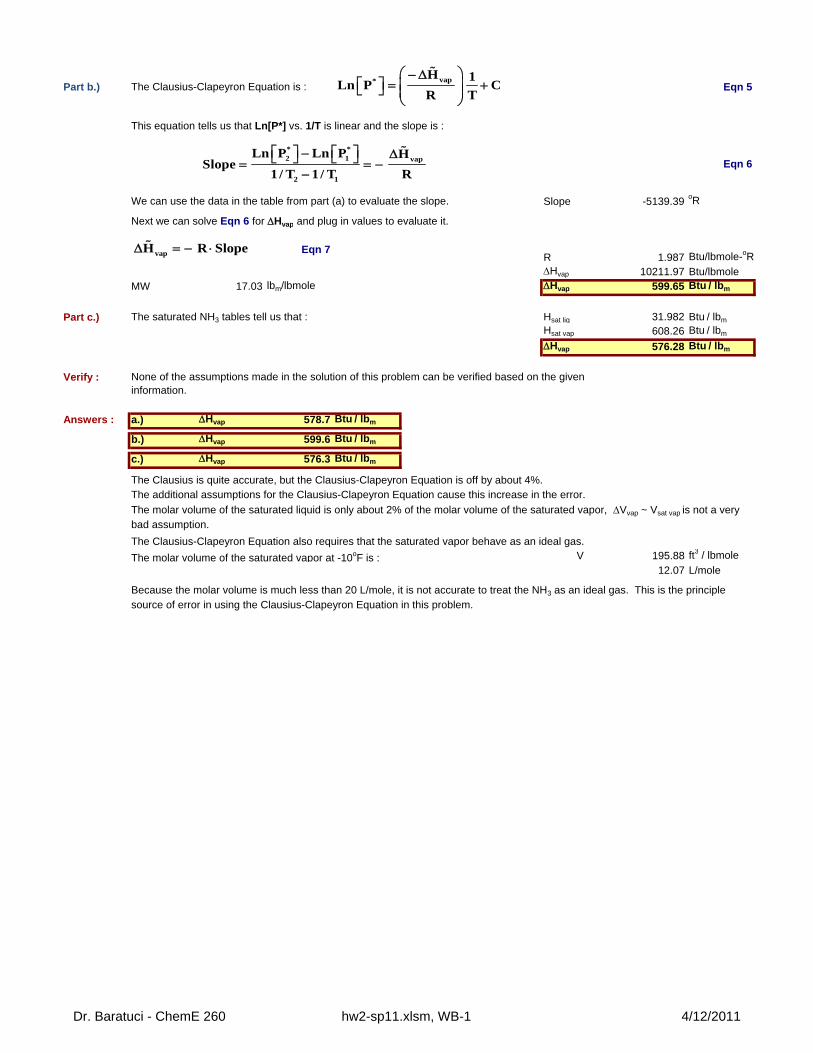
Part b.) The Clausius-Clapeyron Equation is : Eqn 5

This equation tells us that Ln[P*] vs. 1/T is linear and the slope is :

Eqn 6

Slope -5139.39oR

Next we can solve Eqn 6 for Hvap and plug in values to evaluate it.

Eqn 7R 1.987 Btu/lbmole-oRHvap 10211.97 Btu/lbmole

MW 17.03 lbm/lbmole Hvap 599.65 Btu / lbm

Part c.) The saturated NH3 tables tell us that : Hsat liq 31.982 Btu / lbm

Hsat vap 608.26 Btu / lbm

Hvap 576.28 Btu / lbm

Verify :

Answers : a.) Hvap 578.7 Btu / lbm

b.) Hvap 599.6 Btu / lbm

c.) Hvap 576.3 Btu / lbm

The Clausius is quite accurate, but the Clausius-Clapeyron Equation is off by about 4%.The additional assumptions for the Clausius-Clapeyron Equation cause this increase in the error.

The Clausius-Clapeyron Equation also requires that the saturated vapor behave as an ideal gas.

The molar volume of the saturated vapor at -10oF is : V 195.88 ft3 / lbmole

12.07 L/mole

The molar volume of the saturated liquid is only about 2% of the molar volume of the saturated vapor, Vvap ~ Vsat vap is not a very bad assumption.

Because the molar volume is much less than 20 L/mole, it is not accurate to treat the NH3 as an ideal gas. This is the principle source of error in using the Clausius-Clapeyron Equation in this problem.


We can use the data in the table from part (a) to evaluate the slope.

vap*H 1

Ln P CR T

* *2 1 vap

2 1

Ln P Ln P HSlope

1/ T 1/ T R

vapH R Slope


BaratuciHW #2

Problem : WB-2 - Hypothetical Process Paths and the Latent Heat of Vaporization - 8 pts 14-Apr-11

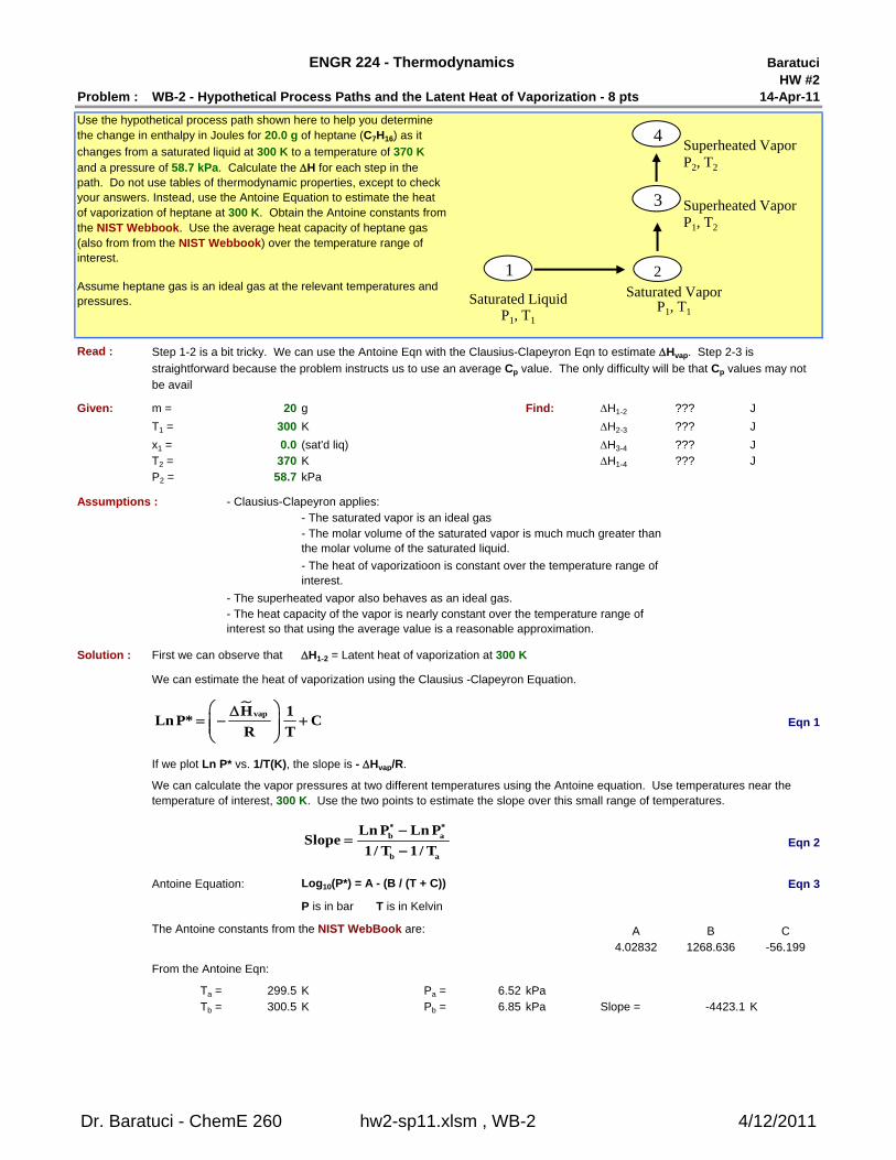
Read :

Given: m = 20 g Find: H1-2 ??? J

T1 = 300 K H2-3 ??? J

x1 = 0.0 (sat'd liq) H3-4 ??? JT2 = 370 K H1-4 ??? JP2 = 58.7 kPa

Assumptions : - Clausius-Clapeyron applies:- The saturated vapor is an ideal gas

- The superheated vapor also behaves as an ideal gas.

Solution : First we can observe that H1-2 = Latent heat of vaporization at 300 K

We can estimate the heat of vaporization using the Clausius -Clapeyron Equation.

Eqn 1

If we plot Ln P* vs. 1/T(K), the slope is - Hvap/R.

Eqn 2

Antoine Equation: Log10(P*) = A - (B / (T + C)) Eqn 3

P is in bar T is in Kelvin

The Antoine constants from the NIST WebBook are: A B C4.02832 1268.636 -56.199

From the Antoine Eqn:

Ta = 299.5 K Pa = 6.52 kPaTb = 300.5 K Pb = 6.85 kPa Slope = -4423.1 K


- The heat capacity of the vapor is nearly constant over the temperature range of interest so that using the average value is a reasonable approximation.

- The molar volume of the saturated vapor is much much greater than the molar volume of the saturated liquid.

- The heat of vaporizatioon is constant over the temperature range of interest.

Step 1-2 is a bit tricky. We can use the Antoine Eqn with the Clausius-Clapeyron Eqn to estimate Hvap. Step 2-3 is

straightforward because the problem instructs us to use an average Cp value. The only difficulty will be that Cp values may not be avail

Assume heptane gas is an ideal gas at the relevant temperatures and pressures.

Use the hypothetical process path shown here to help you determine the change in enthalpy in Joules for 20.0 g of heptane (C7H16) as it

changes from a saturated liquid at 300 K to a temperature of 370 K and a pressure of 58.7 kPa. Calculate the H for each step in the path. Do not use tables of thermodynamic properties, except to check your answers. Instead, use the Antoine Equation to estimate the heat of vaporization of heptane at 300 K. Obtain the Antoine constants from the NIST Webbook. Use the average heat capacity of heptane gas (also from from the NIST Webbook) over the temperature range of interest.

We can calculate the vapor pressures at two different temperatures using the Antoine equation. Use temperatures near the temperature of interest, 300 K. Use the two points to estimate the slope over this small range of temperatures.

Saturated LiquidP1, T1

1 2

3

Saturated VaporP1, T1

Superheated VaporP1, T2

4Superheated VaporP2, T2

vapH 1

Ln P* CR T

b a

b a

Ln P Ln PSlope

1/ T 1/ T

Dr. Baratuci - ChemE 260 hw2-sp11.xlsm , WB-2 4/12/2011

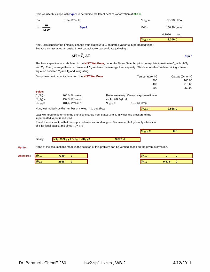
Next we use this slope with Eqn 1 to determine the latent heat of vaporization at 300 K :

R = 8.314 J/mol K Hvap = 36773 J/mol

Eqn 4 MW = 100.20 g/mol

n 0.1996 mol

H(1-2) = 7,340 J

Next, let's consider the enthalpy change from states 2 to 3, saturated vapor to superheated vapor:Because we assumed a constant heat capacity, we can evaluate H using:

Eqn 5

Gas phase heat capacity data from the NIST WebBook: Temperature (K) Cp,gas (J/mol*K)300 165.98400 210.66500 252.09

Solve:Cp(T1) = 166.0 J/mole-KCp(T2) = 197.3 J/mole-KCp, avg = 181.6 J/mole-K H(2-3) = 12,713 J/mol

Now, just multiply by the number of moles, n, to get H2-3 : H(2-3) = 2,538 J

H(3-4) = 0 J

Finally: H1-4 = H1-2 + H2-3 + H3-4 = 9,878 J

Verify :

Answers : H1-2 7340 J H3-4 0 J

H2-3 2538 J H1-4 9,878 J


Last, we need to determine the enthalpy change from states 3 to 4, in which the pressure of the superheated vapor is reduced.

Recall the assumption that the vapor behaves as an ideal gas. Because enthalpy is only a function of T for ideal gases, and since T3 = T4 :

There are many different ways to estimate Cp(T1) and Cp(T2).

The heat capacities are tabulated in the NIST WebBook, under the Name Search option. Interpolate to estimate Cp at both T1

and T2. Then, average these two values of Cp to obtain the average heat capacity. This is equivalent to determining a linear

equation between T1 and T2 and integrating.

pH C T

mn

MW

Dr. Baratuci - ChemE 260 hw2-sp11.xlsm , WB-2 4/12/2011

BaratuciHW #2

Problem : WB-3 - Work and Heat Transfer for a Closed, 3-Step Cycle - 6 pts 14-Apr-11

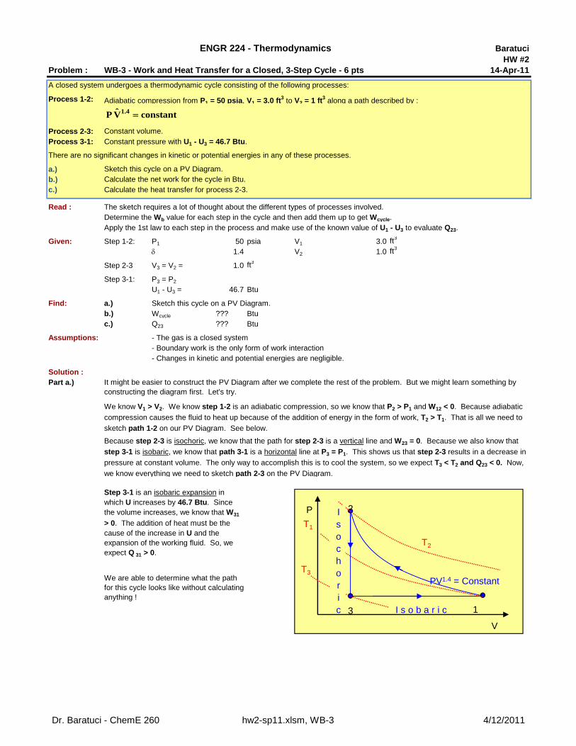
A closed system undergoes a thermodynamic cycle consisting of the following processes:

Process 1-2: Adiabatic compression from P1 = 50 psia, V1 = 3.0 ft3 to V2 = 1 ft3 along a path described by :

Process 2-3: Constant volume.Process 3-1: Constant pressure with U1 - U3 = 46.7 Btu.

There are no significant changes in kinetic or potential energies in any of these processes.

a.) Sketch this cycle on a PV Diagram.b.) Calculate the net work for the cycle in Btu.c.) Calculate the heat transfer for process 2-3.

Read : The sketch requires a lot of thought about the different types of processes involved.Determine the Wb value for each step in the cycle and then add them up to get Wcycle.

Given: Step 1-2: P1 50 psia V1 3.0 ft3

1.4 V2 1.0 ft3

Step 2-3 V3 = V2 = 1.0 ft3

Step 3-1: P3 = P2

U1 - U3 = 46.7 Btu

Find: a.) Sketch this cycle on a PV Diagram.b.) Wcycle ??? Btuc.) Q23 ??? Btu

Assumptions: - The gas is a closed system- Boundary work is the only form of work interaction- Changes in kinetic and potential energies are negligible.

Solution :Part a.)


Apply the 1st law to each step in the process and make use of the known value of U1 - U3 to evaluate Q23.

It might be easier to construct the PV Diagram after we complete the rest of the problem. But we might learn something by constructing the diagram first. Let's try.

We know V1 > V2. We know step 1-2 is an adiabatic compression, so we know that P2 > P1 and W12 < 0. Because adiabatic

compression causes the fluid to heat up because of the addition of energy in the form of work, T2 > T1. That is all we need to

sketch path 1-2 on our PV Diagram. See below.

Because step 2-3 is isochoric, we know that the path for step 2-3 is a vertical line and W23 = 0. Because we also know that

step 3-1 is isobaric, we know that path 3-1 is a horizontal line at P3 = P1. This shows us that step 2-3 results in a decrease in

pressure at constant volume. The only way to accomplish this is to cool the system, so we expect T3 < T2 and Q23 < 0. Now,

we know everything we need to sketch path 2-3 on the PV Diagram.

Step 3-1 is an isobaric expansion in which U increases by 46.7 Btu. Since the volume increases, we know that W31

> 0. The addition of heat must be the cause of the increase in U and the expansion of the working fluid. So, we expect Q 31 > 0.

We are able to determine what the path for this cycle looks like without calculating anything !

1.4ˆP V constant

P

V

1

2

3 I s o b a r i c

PV1.4 = Constant

T1

T2

T3

Isochoric


Part b.)

Eqn 1

All we need to do is determine P2 and then we can use Eqn 1 to evaluate W12.The way to go here is to evaluate the constant, C, from P1 and V1 :

Eqn 2

C 232.777 psia-ft3

Now, apply the polytropic path equation to state 2, as follows.

Eqn 3 Eqn 4

P2 232.8 psia

Now, we can plug values back into Eqn 1 to determine W12 :

1 ft2 144 in2W12 -206.94 psia-ft3

1 Btu 778.17 ft-lbf -38.295 Btu

Step 2-3 is isochoric, so there is no baoundary work: W23 0 Btu

Step 3-1 is isobaric, so we can evaluate W23 from :

Eqn 5

Here, P is either P1 or P3, because they are the same.Plugging in values yields : W31 100.00 psia-ft3

18.505 Btu

Now, we add up the work terms to get : Wcycle = -19.79 Btu

Part c.) In order to determine Q23, we need to apply the 1st Law to the step.

Q23 - W23 = U3 - U2 = 0 Eqn 6

But, W23 = 0, so Eqn 6 becomes : Q23 = U3 - U2 Eqn 7

Next, let's apply the 1st Law to step 1-2. Q12 - W12 = U2 - U1 Eqn 8

Plugging in the value of W12 yields : U2 - U1 = 38.295 Btu

We were given that : U1 - U3 = 46.7 Btu

Therefore : U3 - U2 = - ( U2 - U1 ) - ( U1 - U3 ) Eqn 9

Therefore : U3 - U2 = -84.995 BtuQ23 -84.995 Btu


Answers : a.) See the PV Diagram, above.

b.) Wcycle -19.79 Btu

Applying the 1st Law to step 3-1 yields : Q31 65.205 Btu

COPHP 3.29

What kind of cycle is this ? This is a refrigeration or heat pump cycle because Wcycle < 0. For a cycle, Qcycle = Wcycle, so Qcycle

< 0 as well. The cycle rejects all the heat that is absorbs plus it converts a net amount of input work into heat and also rejects that energy as heat. We cannot tell whether it is a refrigeration or heat pump cycle because the only difference is the goal or desired quantity. If this cycle were a refrigerator, the goal would be to absorb Q23 from the refrigerated space. If the cycle

were a heat pump, the goal would be to reject Q31 to the heated space. Notice that more energy would be removed from the

refrigerated space than the net amount of work put into the cycle. If this cycle were a heat pump, it would deliver Q31 to the

heated space and Q31 is MUCH larger than Wcycle. This advantage is why heat pumps are ofter preferred to electrical

resistance heaters.

In step 1-2: P V = C. We can use V or specific V here because the system is closed and the mass inside is constant. The boundary work for a polytropic process is :

Since Wcycle = W12 + W23 + W31, we will work our way around the cycle and calculate each work term along the way.

2 22 2 1 1

121 1

P V P VdVW P dV C

1V

1 1P V C

2 2P V C 22

CP

V

1 1

31 1 33 3

W PdV P dV P V V P V


BaratuciHW #2

Problem : WB-4 - Heat Conduction Through a Composite Wall - 3 pts 14-Apr-11

Brick InsulationData : k 1.4 0.05 Btu/h-ft-oR

Read : This problem is an application of Fourier's Law of Conduction.

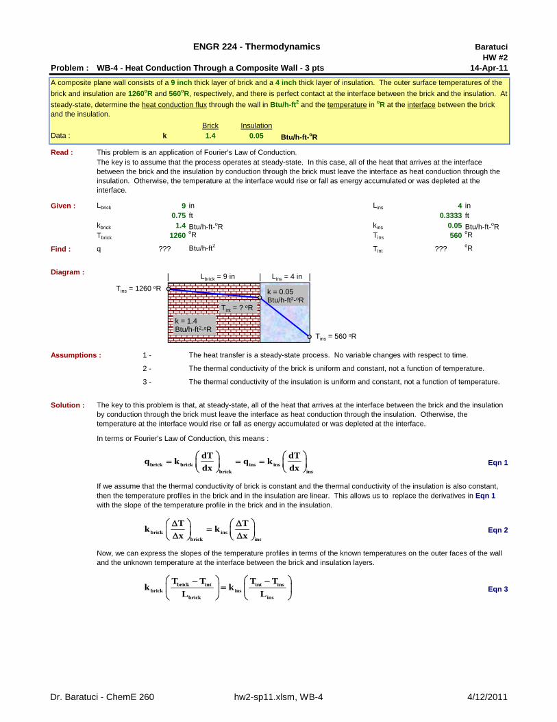
Given : Lbrick 9 in Lins 4 in0.75 ft 0.3333 ft

kbrick 1.4 Btu/h-ft-oR kins 0.05 Btu/h-ft-oRTbrick 1260

oR Tins 560oR

Find : q ??? Btu/h-ft2 Tint ???oR

Diagram :

Assumptions : 1 -

2 -

3 -

Solution :

In terms or Fourier's Law of Conduction, this means :

Eqn 1

Eqn 2

Eqn 3


A composite plane wall consists of a 9 inch thick layer of brick and a 4 inch thick layer of insulation. The outer surface temperatures of the

brick and insulation are 1260oR and 560oR, respectively, and there is perfect contact at the interface between the brick and the insulation. At

steady-state, determine the heat conduction flux through the wall in Btu/h-ft2 and the temperature in oR at the interface between the brick and the insulation.

If we assume that the thermal conductivity of brick is constant and the thermal conductivity of the insulation is also constant, then the temperature profiles in the brick and in the insulation are linear. This allows us to replace the derivatives in Eqn 1 with the slope of the temperature profile in the brick and in the insulation.

Now, we can express the slopes of the temperature profiles in terms of the known temperatures on the outer faces of the wall and the unknown temperature at the interface between the brick and insulation layers.

The key is to assume that the process operates at steady-state. In this case, all of the heat that arrives at the interface between the brick and the insulation by conduction through the brick must leave the interface as heat conduction through the insulation. Otherwise, the temperature at the interface would rise or fall as energy accumulated or was depleted at the interface.

The heat transfer is a steady-state process. No variable changes with respect to time.

The thermal conductivity of the brick is uniform and constant, not a function of temperature.

The thermal conductivity of the insulation is uniform and constant, not a function of temperature.

The key to this problem is that, at steady-state, all of the heat that arrives at the interface between the brick and the insulation by conduction through the brick must leave the interface as heat conduction through the insulation. Otherwise, the temperature at the interface would rise or fall as energy accumulated or was depleted at the interface.

Lbrick = 9 in Lins = 4 in

k = 1.4Btu/h-ft2-oR

k = 0.05Btu/h-ft2-oR

Tins = 560 oR

Tins = 1260 oR

Tint = ? oR

brick brick ins insbrick ins

dT dTq k q k

dx dx

brick insbrick ins

T Tk k

x x

brick int int insbrick ins

brick ins

T T T Tk k

L L


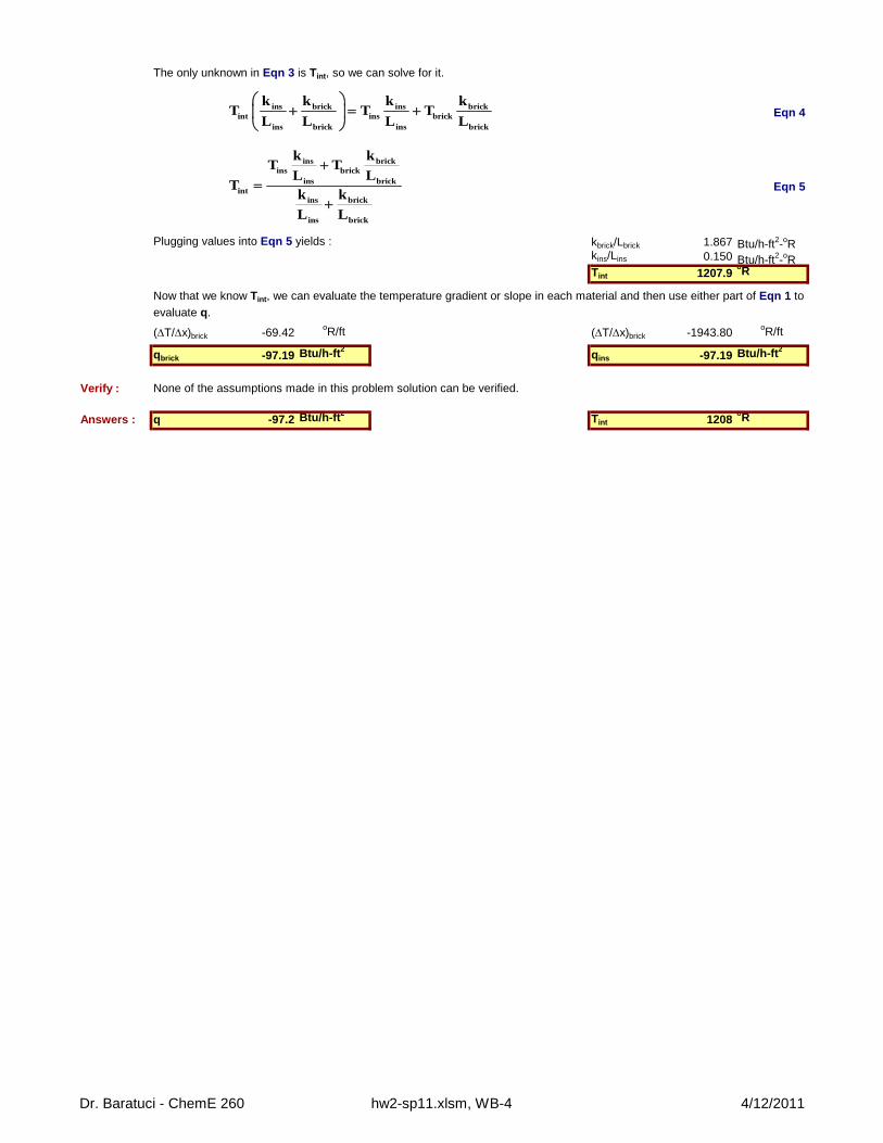
The only unknown in Eqn 3 is Tint, so we can solve for it.

Eqn 4

Eqn 5

Plugging values into Eqn 5 yields : kbrick/Lbrick 1.867 Btu/h-ft2-oRkins/Lins 0.150 Btu/h-ft2-oRTint 1207.9

oR

(T/x)brick -69.42oR/ft (T/x)brick -1943.80

oR/ft

qbrick -97.19 Btu/h-ft2qins -97.19 Btu/h-ft2


Answers : q -97.2 Btu/h-ft2Tint 1208

oR

Now that we know Tint, we can evaluate the temperature gradient or slope in each material and then use either part of Eqn 1 to

evaluate q.

ins brick ins brickint ins brick

ins brick ins brick

k k k kT T T

L L L L

ins brickins brick

ins brickint

ins brick

ins brick

k kT T

L LT

k k

L L


BaratuciHW #2

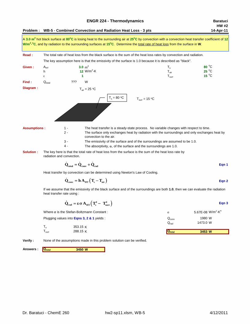
Problem : WB-5 - Combined Convection and Radiation Heat Loss - 3 pts 14-Apr-11

Read :

Given : AHT 3.0 m2 Ts 80oC

h 12 W/m2-K Tair 25oC

1 Tsurr 15oC

Find : Qtotal ??? W

Diagram :

Assumptions : 1 -2 -

3 -4 - The absorptivity, , of the surface and the surroundings are 1.0.

Solution :

Eqn 1

Heat transfer by convection can be determined using Newton's Law of Cooling.

Eqn 2

Eqn 3

Where is the Stefan-Boltzmann Constant : 5.67E-08 W/m2-K4

Plugging values into Eqns 3, 2 & 1 yields : Qconv 1980 WQrad 1473.0 W

Ts 353.15 KTsurr 288.15 K Qtotal 3453 W


Answers : Qtotal 3450 W

The emissivity of the surface and of the surroundings are assumed to be 1.0.

The surface only exchanges heat by radiation with the surroundings and only exchanges heat by convection to the air.

If we assume that the emissivity of the black surface and of the surroundings are both 1.0, then we can evaluate the radiation heat transfer rate using :


The key here is that the total rate of heat loss from the surface is the sum of the heat loss rate by radiation and convection.

A 3.0 m2 hot black surface at 80oC is losing heat to the surrounding air at 25oC by convection with a convection heat transfer coefficient of 12

W/m2-oC, and by radiation to the surrounding surfaces at 15oC. Determine the total rate of heat loss from the surface in W.

The total rate of heat loss from the black surface is the sum of the heat loss rates by convection and radiation.

The key assumption here is that the emissivity of the surface is 1.0 because it is described as "black".

The heat transfer is a steady-state process. No variable changes with respect to time.

Tsurr = 15 oC

Tair = 25 oC

Ts = 80 oC

total conv radQ Q Q

conv HT s airQ h A T T

4 4rad HT s surrQ A T T


BaratuciHW #2

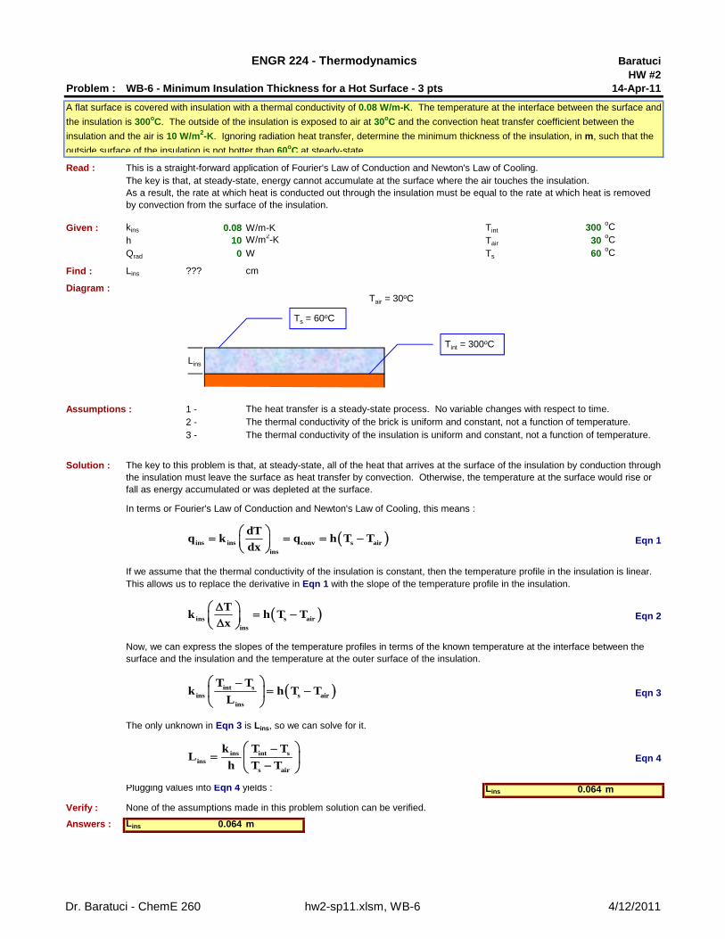
Problem : WB-6 - Minimum Insulation Thickness for a Hot Surface - 3 pts 14-Apr-11

Read : This is a straight-forward application of Fourier's Law of Conduction and Newton's Law of Cooling.

Given : kins 0.08 W/m-K Tint 300oC

h 10 W/m2-K Tair 30oC

Qrad 0 W Ts 60oC

Find : Lins ??? cm

Diagram :

Assumptions : 1 -2 -3 -

Solution :

In terms or Fourier's Law of Conduction and Newton's Law of Cooling, this means :

Eqn 1

Eqn 2

Eqn 3

The only unknown in Eqn 3 is Lins, so we can solve for it.

Eqn 4

Plugging values into Eqn 4 yields : Lins 0.064 m


Answers : Lins 0.064 m

Now, we can express the slopes of the temperature profiles in terms of the known temperature at the interface between the surface and the insulation and the temperature at the outer surface of the insulation.

The key is that, at steady-state, energy cannot accumulate at the surface where the air touches the insulation.As a result, the rate at which heat is conducted out through the insulation must be equal to the rate at which heat is removed by convection from the surface of the insulation.

The thermal conductivity of the insulation is uniform and constant, not a function of temperature.

The key to this problem is that, at steady-state, all of the heat that arrives at the surface of the insulation by conduction through the insulation must leave the surface as heat transfer by convection. Otherwise, the temperature at the surface would rise or fall as energy accumulated or was depleted at the surface.

If we assume that the thermal conductivity of the insulation is constant, then the temperature profile in the insulation is linear. This allows us to replace the derivative in Eqn 1 with the slope of the temperature profile in the insulation.


A flat surface is covered with insulation with a thermal conductivity of 0.08 W/m-K. The temperature at the interface between the surface and

the insulation is 300oC. The outside of the insulation is exposed to air at 30oC and the convection heat transfer coefficient between the

insulation and the air is 10 W/m2-K. Ignoring radiation heat transfer, determine the minimum thickness of the insulation, in m, such that the

outside surface of the insulation is not hotter than 60oC at steady-state

The heat transfer is a steady-state process. No variable changes with respect to time.The thermal conductivity of the brick is uniform and constant, not a function of temperature.

Lins

Tint = 300oC

Ts = 60oC

Tair = 30oC

ins ins conv s airins

dTq k q h T T

dx

ins s airins

Tk h T T

x

int sins s air

ins

T Tk h T T

L

ins int sins

s air

k T TL

h T T


BaratuciHW #2

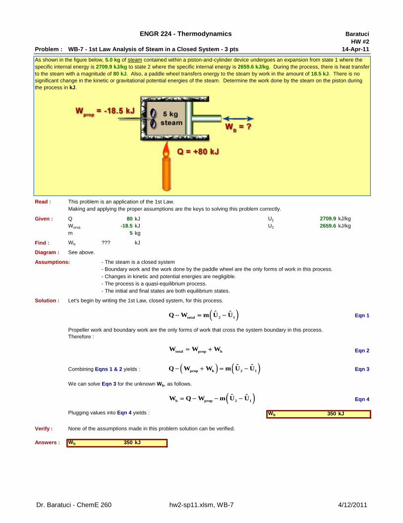
Problem : WB-7 - 1st Law Analysis of Steam in a Closed System - 3 pts 14-Apr-11

Read : This problem is an application of the 1st Law.Making and applying the proper assumptions are the keys to solving this problem correctly.

Given : Q 80 kJ U1 2709.9 kJ/kgWprop -18.5 kJ U2 2659.6 kJ/kgm 5 kg

Find : Wb ??? kJ

Diagram : See above.

Assumptions: - The steam is a closed system

- Changes in kinetic and potential energies are negligible.- The process is a quasi-equilibrium process.- The initial and final states are both equilibrium states.

Solution : Let's begin by writing the 1st Law, closed system, for this process.

Eqn 1

Eqn 2

Combining Eqns 1 & 2 yields : Eqn 3

We can solve Eqn 3 for the unknown Wb, as follows.

Eqn 4

Plugging values into Eqn 4 yields : Wb 350 kJ


Answers : Wb 350 kJ


As shown in the figure below, 5.0 kg of steam contained within a piston-and-cylinder device undergoes an expansion from state 1 where the specific internal energy is 2709.9 kJ/kg to state 2 where the specific internal energy is 2659.6 kJ/kg. During the process, there is heat transfer to the steam with a magnitude of 80 kJ. Also, a paddle wheel transfers energy to the steam by work in the amount of 18.5 kJ. There is no significant change in the kinetic or gravitational potential energies of the steam. Determine the work done by the steam on the piston during the process in kJ.

- Boundary work and the work done by the paddle wheel are the only forms of work in this process.

Propeller work and boundary work are the only forms of work that cross the system boundary in this process.Therefore :

total 2 1ˆ ˆQ W m U U

total prop bW W W

prop b 2 1ˆ ˆQ W W m U U

b prop 2 1ˆ ˆW Q W m U U


BaratuciHW #2

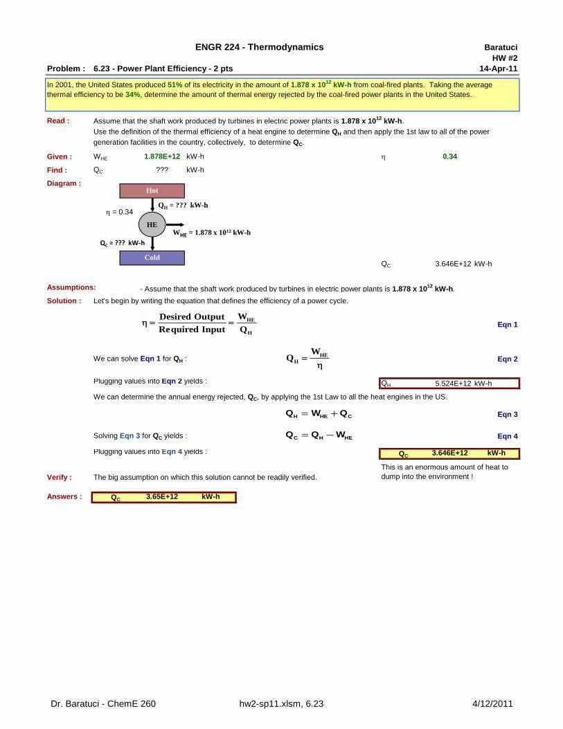
Problem : 6.23 - Power Plant Efficiency - 2 pts 14-Apr-11

Read :

Given : WHE 1.878E+12 kW-h 0.34

Find : QC ??? kW-h

Diagram :

QC 3.646E+12 kW-h

Assumptions:

Solution : Let's begin by writing the equation that defines the efficiency of a power cycle.

Eqn 1

We can solve Eqn 1 for QH : Eqn 2

Plugging values into Eqn 2 yields : QH 5.524E+12 kW-h

We can determine the annual energy rejected, QC, by applying the 1st Law to all the heat engines in the US.

Eqn 3

Solving Eqn 3 for QC yields : Eqn 4

Plugging values into Eqn 4 yields : QC 3.646E+12 kW-h

Verify : The big assumption on which this solution cannot be readily verified.

Answers : QC 3.65E+12 kW-h

This is an enormous amount of heat to dump into the environment !


In 2001, the United States produced 51% of its electricity in the amount of 1.878 x 1012 kW-h from coal-fired plants. Taking the average thermal efficiency to be 34%, determine the amount of thermal energy rejected by the coal-fired power plants in the United States.

Assume that the shaft work produced by turbines in electric power plants is 1.878 x 1012 kW-h.

Use the definition of the thermal efficiency of a heat engine to determine QH and then apply the 1st law to all of the power

generation facilities in the country, collectively, to determine QC.

- Assume that the shaft work produced by turbines in electric power plants is 1.878 x 1012 kW-h.

Hot

Cold

HE

QH = ??? kW-h

QC = ??? kW‐h

WHE = 1.878 x 1012 kW-h

= 0.34

HE

H

WDesired Output

Required Input Q

HEH

WQ

H HE CQ W Q= +

C H HEQ Q W= -


BaratuciHW #2

Problem : 6.41 - Work, Heat and COP in a Refrigeration Cycle - 2 pts 14-Apr-11

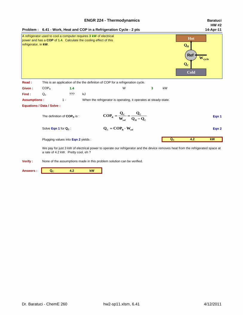
Read : This is an application of the the definiton of COP for a refrigeration cycle.

Given : COPR 1.4 W 3 kW

Find : QC ??? kJ

Assumptions : 1 - When the refrigerator is operating, it operates at steady-state.

Equations / Data / Solve :

The definition of COPR is : Eqn 1

Solve Eqn 1 for QC : Eqn 2

Plugging values into Eqn 2 yields : QC 4.2 kW


Answers : QC 4.2 kW


A refrigerator used to cool a computer requires 3 kW of electrical power and has a COP of 1.4. Calculate the cooling effect of this refrigerator, in kW.

We pay for just 3 kW of electrical power to operate our refrigerator and the device removes heat from the refrigerated space at a rate of 4.2 kW. Pretty cool, eh ?

Ref

Hot

Cold

QH

QC

Wcycle

C CR

ref H C

Q QCOP

W Q Q

C R refQ COP W


BaratuciHW #2

Problem : 6.55 - Heat Pump COP and Monthly Operating Cost - 2 pts 14-Apr-11

Read :

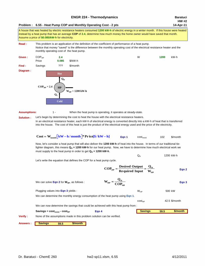
Given : COPHP 2.4 W 1200 kW-hPrice 0.085 $/kW-h

Find : Savings ??? $/month

Diagram :

Assumptions: 1 - When the heat pump is operating, it operates at steady-state.

Solution :

Eqn 1 costresist 102 $/month

QH 1200 kW-h

Let's write the equation that defines the COP for a heat pump cycle.

Eqn 2

We can solve Eqn 2 for WHP, as follows : Eqn 3

Plugging values into Eqn 3 yields : WHP 500 kW

costHP 42.5 $/month

Savings = costresist - costHP Eqn 4 Savings 59.5 $/month


Answers : Savings 59.5 $/month

We can determine the monthly energy consumption of the heat pump using Eqn 1.

We can now determine the savings that could be achieved with this heat pump from :


A house that was heated by electric resistance heaters consumed 1200 kW-h of electric energy in a winter month. If this house were heated instead by a heat pump that has an average COP of 2.4, determine how much money the home owner would have saved that month. Assume a price of $0.085/kW-h for electricity.

This problem is an application of the definition of the coefficient of performance of a heat pump.Notice that money "saved" is the difference between the monthly operating cost of the electrical resistance heater and the monthly operating cost of the heat pump.

Let's begin by determining the cost to heat the house with the electrical resistance heaters.

In an electrical resistance heater, each kW-h of electrical energy is converted directly into a kW-h of heat that is transferred into the house. The cost of this heat is just the product of the electrical energy used and the price of the electricity.

Now, let's consider a heat pump that will also deliver the 1200 kW-h of heat into the house. In terms of our traditional tie-fighter diagram, this means QH = 1200 kW-h for our heat pump. Now, we have to determine how much electrical work we

must supply to the heat pump in order to get QH = 1200 kW-h.

Hot

Cold

HP

QH

QC

WHP = 1200 kW-h

COPHP = 2.4

HHP

HP

QDesired OutputCOP

Required Input W

HHP

HP

QW

COP

month kW h / montCost W * Pr ich [$ / W h]e k


ENGR 224 - Thermodynamics HW #2 Problem : 3.26 ......Baratuci HW #2 Problem : 3.26 - Steam NIST /...

Documents

Transcript of ENGR 224 - Thermodynamics HW #2 Problem : 3.26 ......Baratuci HW #2 Problem : 3.26 - Steam NIST /...