Engineering Materials Design

Lecture . 2

2Failure Prevention

By

Dr. Mohammed Ramidh

1. Failures Resulting from Static Loading A static load is a stationary force or couple applied to a member. To be

stationary, the force or couple must be unchanging in magnitude, point or points

of application, and direction. A static load can produce axial tension or

compression, a shear load, a bending load, a torsional load, or any combination of

these. To be considered static, the load cannot change in any manner. In this chapter we consider the relations between strength and static

loading in order to make the decisions concerning material and its treatment,

fabrication, and geometry for satisfying the requirements of functionality, safety,

reliability, competitiveness, usability, manufacturability, and marketability. How

far we go down this list is related to the scope of the examples. ―Failure‖ is the first word in the chapter title. Failure can mean a part has

separated into two or more pieces; has become permanently distorted, thus

ruining its geometry; has had its reliability downgraded; or has had its function

compromised, whatever the reason.

Stress Concentration

Stress concentration is a highly localized effect. In some instances it may be

due to a surface scratch. If the material is ductile and the load static, the design

load may cause yielding in the critical location in the notch. This yielding can

involve strain strengthening of the material and an increase in yield strength at

the small critical notch location. Since the loads are static and the material is

ductile, that part can carry the loads satisfactorily with no general yielding. In

these cases the designer sets the geometric (theoretical) stress concentration

factor Kt to unity.

When using this rule for ductile materials with static loads, be careful to

assure yourself that the material is not susceptible to brittle fracture in the

environment of use.

Brittle materials do not exhibit a plastic range. A brittle material ―feels‖ the

stress concentration factor Kt or Kts.

An exception to this rule is a brittle material that inherently contains

microdiscontinuity stress concentration, worse than the macrodiscontinuity that

the designer has in mind. Sand molding introduces sand particles, air, and water

vapor bubbles. The grain

structure of cast iron contains graphite flakes (with little strength), which are

literally cracks introduced during the solidification process. When a tensile test

on a cast iron is performed, the strength reported in the literature includes this

stress concentration. In such cases Kt or Kts need not be applied.

1-1. Failure Theories

Unfortunately, there is no universal theory of failure for the general case of

material properties and stress state. Instead, over the years several hypotheses

have been formulated and tested, leading to today’s accepted practices. Being

accepted, we will characterize these ―practices‖ as theories as most designers do.

Structural metal behavior is typically classified as being ductile or brittle,

although under special situations, a material normally considered ductile can fail

in a brittle manner. Ductile materials are normally classified such that ≥ 0.05

and have an identifiable yield strength that is often the same in compression as in

tension ( = = ). Brittle materials, < 0.05, do not exhibit an

identifiable yield strength, and are typically classified by ultimate tensile and

compressive strengths, and, respectively (where is given as a

positive quantity). The generally accepted theories are:

Ductile materials (yield criteria)

• Maximum shear stress (MSS),

• Distortion energy (DE),

• Ductile Coulomb-Mohr (DCM),

Brittle materials (fracture criteria)

• Maximum normal stress (MNS),

• Brittle Coulomb-Mohr (BCM),

• Modified Mohr (MM),

Ductile materials (yield criteria)

1-2. Maximum-Shear-Stress Theory for Ductile Materials

The maximum-shear-stress theory predicts that yielding begins

whenever the maximum shear stress in any element equals or

exceeds the maximum shear stress in a tensiontest specimen of the

same material when that specimen begins to yield.

the maximum-shear-stress theory predicts yielding when

…………(2-1)

Where is the yielding stress, and n is the factor of safety.

Note that this implies that the yield strength in shear is given by

………… (2-2) The MSS theory is also referred to as the Tresca or Guest theory.

1-3 Distortion-Energy Theory for Ductile Materials

The distortion-energy theory predicts that yielding occurs when the

distortion strain energy per unit volume reaches or exceeds the

distortion strain energy per unit volume for yield in simple tension

or compression of the same material.

The distortion-energy theory is also called:

• The von Mises or von Mises–Hencky theory

• The shear-energy theory

• The octahedral-shear-stress theory

The distortion-energy theory predicts yielding when

……………… (2-3)

Where is usually called the von Mises stress, named after Dr. R.

von Mises, who contributed to the theory. where the von Mises

stress is

√

………….. (2-4)

the shear yield strength predicted by the distortion-energy theory is

………… (2-5)

EXAMPLE 3–1:

A hot-rolled steel has a yield strength of Syt =Syc = 100 kpsi and a true

strain at fracture of εf = 0.55. Estimate the factor of safety for the

following principal stress states:

(a) 70, 70, 0 kpsi.

(b) 30, 70, 0 kpsi.

(c) 0, 70, −30 kpsi.

(d) 0, −30, −70 kpsi.

(e) 30, 30, 30 kpsi.

Solution :

Since εf > 0.05 and Syc and Syt are equal, the material is ductile

and the distortion energy (DE) theory applies. The maximum-shear-

stress (MSS) theory will also be applied and compared to the DE

results. Note that cases a to d are plane stress states.

(a) The ordered principal stresses are σ1 = 70,σ2 = 70, σ3 = 0

kpsi.

DE : From Eqs. (2-3) and (2-4).

√

= 70 kpsi

=

MSS : From Eq. (2-1) with a factor of safety,

=

(b) The ordered principal stresses are σ1 = 70,σ2 = 30, σ3 = 0

kpsi.

DE: From Eqs. (2-3) and (2-4).

√

= 60.8 kpsi

=

MSS: From Eq. (2-1)

=

(c) The ordered principal stresses are σ1 = 70,σ2 = 0,σ3 = −30 kpsi.

DE : From Eqs. (2-3) and (2-4).

√

= 88.9 kpsi

=

MSS: From Eq. (2-1),

=

(d) The ordered principal stresses are σ1 = 0,σ2 = −30,σ3 = −70 kpsi.

DE: From Eqs. (2-3) and (2-4).

√

= 60.8 kpsi

=

MSS: From Eq. (2-1),

=

(e) The ordered principal stresses are σ1 = 30,σ2 = 30,σ3 = 30 kpsi

DE: From Eqs. (2-3) and (2-4).

√

= 0

=

MSS: From Eq. (2-1),

=

A tabular summary of the factors of safety is included for comparisons.

1–4 Coulomb-Mohr Theory for Ductile Materials

A variation of Mohr’s theory, called the Coulomb-Mohr theory or the

internal-friction theory,

Not all materials have compressive strengths equal to their corresponding

tensile values. For example, the yield strength of magnesium alloys in

compression may be as little as 50 percent of their yield strength in

tension. The ultimate strength of gray cast irons in compression varies

from 3 to 4 times greater than the ultimate tensile strength. So, in this

section, we are primarily interested in those theories that can be used to

predict failure for materials whose strengths in tension and compression

are not equal.

This is can be expressed as a design equation with a factor of safety ,n ,

can be written as.

………….( 2-6 )

Where either yield strength or ultimate strength can be used.

The torsional yield strength occurs when = . Then

…………… (2-7)

EXAMPLE 4–1 A 25-mm-diameter shaft is statically torqued to 230 N ? m. It is

made of cast 195-T6 aluminum, with a yield strength in tension of

160 MPa and a yield strength in compression of 170 MPa. It is

machined to final diameter. Estimate the factor of safety of the shaft.

Solution The maximum shear stress is given by

The two nonzero principal stresses are 75 and −75 MPa, making the

ordered principal stresses σ1 = 75, σ2 = 0, and σ3 = −75 MPa.

From Eq. (2–6), for yield,

EXAMPLE 4–2

This example illustrates the use of a failure theory to determine the

strength of a mechanical element or component. The example may

also clear up any confusion existing between the phrases strength of

a machine part, strength of a material, and strength of a part at a

point.

A certain force F applied at D near the end of the 15-in lever shown

in Fig.(1-1) , which is quite similar to a socket wrench, results in

certain stresses in the cantilevered bar OABC. This bar (OABC) is of

AISI 1035 steel, forged and heat-treated so that it has a minimum

(ASTM) yield strength of 81 kpsi. We presume that this component

would be of no value after yielding. Thus the force F required to

initiate yielding can be regarded as the strength of the component

part. Find this force.

Figure 1–1

Solution We will assume that lever DC is strong enough and hence not a

part of the problem. A 1035 steel, heat-treated, will have a reduction in

area of 50 percent or more and hence is a ductile material at normal

temperatures. This also means that stress concentration at shoulder A need

not be considered. A stress element at A on the top surface will be

subjected to a tensile bending stress and a torsional stress. This point, on

the 1-in-diameter section, is the weakest section, and governs the strength

of the assembly. The two stresses are

the distortion-energy theory, we find, from lower Eq. or Eq. (2-4)

Eq. (2-3) , then

the MSS theory, Eq.

or from lower Eq.

Brittle materials (fracture criteria)

1–5 Maximum-Normal-Stress Theory for Brittle Materials The maximum-normal-stress (MNS) theory states that failure occurs

whenever one of the three principal stresses equals or exceeds the

strength. Again we arrange the principal stresses for a general stress

state in the ordered form σ1 ≥ σ2 ≥ σ3. This theory then predicts

that failure occurs whenever

……….(2-8)

where Sut and Suc are the ultimate tensile and compressive strengths,

respectively, given as positive quantities.

For

For

1–6 Modifications of the Mohr Theory for Brittle Materials We will discuss two modifications of the Mohr theory for brittle materials:

the Brittle-Coulomb-Mohr (BCM) theory and the modified Mohr (MM)

theory. The equations provided for the theories will be restricted to plane

stress and be of the design type incorporating the factor of safety.

Brittle-Coulomb-Mohr (BCM)

For 2-9a

For 2-9b

For 2-9c

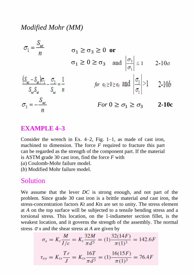
Modified Mohr (MM)

or

For 2-10c

EXAMPLE 4–3

Consider the wrench in Ex. 4–2, Fig. 1–1, as made of cast iron,

machined to dimension. The force F required to fracture this part

can be regarded as the strength of the component part. If the material

is ASTM grade 30 cast iron, find the force F with

(a) Coulomb-Mohr failure model.

(b) Modified Mohr failure model.

Solution

We assume that the lever DC is strong enough, and not part of the

problem. Since grade 30 cast iron is a brittle material and cast iron, the

stress-concentration factors Kt and Kts are set to unity. The stress element

at A on the top surface will be subjected to a tensile bending stress and a

torsional stress. This location, on the 1-indiameter section fillet, is the

weakest location, and it governs the strength of the assembly. The normal

stress σx and the shear stress at A are given by

From Eq. (6) the nonzero principal stresses and are

, =

(a) For BCM, Eq. (2–9b) applies with n = 1 for failure.

(b) For MM, the slope of the load line is Then , Eq. (2–10a) applies. ,

1–7 Selection of Failure Criteria For ductile behavior the preferred criterion is the distortion-energy

theory, although some designers also apply the maximum-shear-

stress theory because of its simplicity and conservative nature. In the

rare case when Syt = Syc , the ductile Coulomb-Mohr method is

employed.

For brittle behavior, the original Mohr hypothesis, constructed with

tensile, compression, and torsion tests, with a curved failure locus is

the best hypothesis we have. However, the difficulty of applying it

without a computer leads engineers to choose modifications, namely,

Coulomb Mohr, or modified Mohr. A lower Figure provides a

summary flowchart for the selection of an effective procedure for

analyzing or predicting failures from static loading for brittle or

ductile behavior.

Homework 1. A ductile hot-rolled steel bar has a minimum yield strength in

tension and compression of 50 kpsi. Using the distortion-energy and

maximum-shear-stress theories determine the factors of safety for

the following plane stress states: (a) σx = 12 kpsi, σy = 6 kpsi

(b) σx = 12 kpsi, τx y = −8 kpsi

(c) σx = −6 kpsi, σy = −10 kpsi, τx y = −5 kpsi

(d) σx = 12 kpsi, σy = 4 kpsi, τx y = 1 kpsi

2. An ASTM cast iron has minimum ultimate strengths of 30 kpsi in

tension and 100 kpsi in compression. Find the factors of safety using

the MNS, BCM, and MM theories for each of the following stress

states. (a) σx = 20 kpsi, σy = 6 kpsi

(b) σx = 12 kpsi, τx y = −8 kpsi

(c) σx = −6 kpsi, σy = −10 kpsi, τx y = −5 kpsi

(d) σx = −12 kpsi, τx y = 8 kpsi 3. Repeat question, 1 for:

(a) σ1 = 12 kpsi, σ3 = 12 kpsi

(b) σ1 = 12 kpsi, σ3= 6 kpsi

(c) σ1= 12 kpsi, σ3= −12 kpsi

(d) σ1 = −6 kpsi, σ3= −12 kpsi 4. Repeat question, 1 for a bar of AISI 1020 cold-drawn steel and:

(a) σx = 180 MPa, σy = 100 MPa

(b) σx = 180 MPa, τx y = 100 MPa

(c) σx = −160 MPa, τx y = 100 MPa

(d) τx y = 150 MPa 5. Among the decisions a designer must make is selection of the

failure criteria that is applicable to the material and its static loading.

A 1020 hot-rolled steel has the following properties: Sy = 42 kpsi,

Sut = 66.2 kpsi, and true strain at fracture εf = 0.90. estimate the

factor of safety.

(a) σx = 9 kpsi, σy = −5 kpsi.

(b) σx = 12 kpsi, τx y = 3 kpsi ccw.

(c) σx = −4 kpsi, σy = −9 kpsi, τx y = 5 kpsi cw.

(d) σx = 11 kpsi, σy = 4 kpsi, τx y = 1 kpsi cw.

6. This problem illustrates that the factor of safety for a machine

element depends on the particular point selected for analysis. Here

you are to compute factors of safety, based upon the distortion-

energy theory, for stress elements at A and B of the member shown

in the figure. This bar is made of AISI 1006 cold-drawn steel and is

loaded by the forces F = 0.55 kN, P = 8.0 kN, and T = 30 N ? m.

7. The figure shows a crank loaded by a force F = 190 lbf which causes

twisting and bending of the

-in-diameter shaft fixed to a support at the

origin of the reference system. In actuality, the support may be an inertia

which we wish to rotate, but for the purposes of a strength analysis we

can consider this to be a statics problem. The material of the shaft AB is

hot-rolled AISI 1018 steel (Table A–20). Using the maximum-shear-stress

theory, find the factor of safety based on the stress at point A.

8. A light pressure vessel is made of 2024-T3 aluminum alloy

tubing with suitable end closures. This cylinder has a 3 -in OD, a

0.065-in wall thickness, and ν = 0.334. The purchase order

specifies a minimum yield strength of 46 kpsi. What is the factor of

safety if the pressure-release valve is set at 500 psi?

2.Fatigue Failure Resulting from Variable Loading

In this section we shall examine how parts fail under variable loading

and how to proportion them to successfully resist such conditions.

2–1 Introduction to Fatigue In most testing of those properties of materials that relate to the stress-strain

diagram, the load is applied gradually, to give sufficient time for the strain to

fully develop. Furthermore, the specimen is tested to destruction, and so the

stresses are applied only once. Testing of this kind is applicable, to what are

known as static conditions; such conditions closely approximate the actual

conditions to which many structural and machine members are subjected.

The condition frequently arises, however, in which the stresses vary with

time or they fluctuate between different levels. For example, a particular

fiber on the surface of a rotating shaft subjected to the action of bending

loads undergoes both tension and compression for each revolution of the

shaft. If the shaft is part of an electric motor rotating at 1725 rev/min, the

fiber is stressed in tension and compression 1725 times eachminute. If, in

addition, the shaft is also axially loaded (as it would be, for example, by a

helical or worm gear), an axial component of stress is superposed upon the

bending component. In this case, some stress is always present in any one

fiber, but now the level of stress is fluctuating. These and other kinds of

loading occurring in machine members produce stresses that are called

variable, repeated, alternating, or fluctuating stresses.

Often, machine members are found to have failed under the action of

repeated or fluctuating stresses; yet the most careful analysis reveals that the

actual maximum stresses were well below the ultimate strength of the

material, and quite frequently even below the yield strength. The most

distinguishing characteristic of these failures is that the stresses have been

repeated a very large number of times. Hence the failure is called a fatigue

failure. When machine parts fail statically, they usually develop a very large

deflection, because the stress has exceeded the yield strength, and the part is

replaced before fracture actually occurs. Thus many static failures give visible

warning in advance. But a fatigue failure gives no warning! It is sudden and

total, and hence dangerous. It is relatively simple to design against a static

failure, because our knowledge is comprehensive. Fatigue is amuchmore

complicated phenomenon, only partially understood, and the engineer seeking

competence must acquire as much knowledge of the subject as possible. Fatigue failure is due to crack formation and propagation. A fatigue crack

will typically initiate at a discontinuity in the material where the cyclic stress

is a maximum. Discontinuities can arise because of: • Design of rapid changes in cross section, keyways, holes, etc. where

stress concentrations occur.

• Elements that roll and/or slide against each other (bearings, gears, cams,

etc.) under high contact pressure, developing concentrated subsurface

contact stresses that can cause surface pitting or spalling after many cycles

of the load.

• Carelessness in locations of stamp marks, tool marks, scratches, and

burrs; poor joint design; improper assembly; and other fabrication faults.

• Composition of the material itself as processed by rolling, forging,

casting, extrusion, drawing, heat treatment, etc. Microscopic and

submicroscopic surface and subsurface discontinuities arise, such as

inclusions of foreign material, alloy segregation, voids, hard precipitated

particles, and crystal discontinuities. Various conditions that can accelerate crack initiation include residual tensile

stresses, elevated temperatures, temperature cycling, a corrosive environment,

and high-frequency cycling.

Approach to Fatigue Failure in Analysis and Design As noted in the previous section, there are a great many factors to be

considered, even for very simple load cases. The methods of fatigue failure

analysis represent a combination of engineering and science. Often science

fails to provide the complete answers that are needed. But the airplane must

still be made to fly—safely. And the automobile must be manufactured with a

reliability that will ensure a long and troublefree life and at the same time

produce profits for the stockholders of the industry. Thus, while science has

not yet completely explained the complete mechanism of fatigue, the engineer

must still design things that will not fail. In a sense this is a classic example of

the true meaning of engineering as contrasted with science. Engineers use

science to solve their problems if the science is available. But available or not,

the problem must be solved, and whatever form the solution takes under these

conditions is called engineering.

2-2 Fatigue-Life Methods The three major fatigue life methods used in design and analysis are the

stress-life method, the strain-life method, and the linear-elastic fracture

mechanics method.

The Stress-Life Method To determine the strength of materials under the action of fatigue loads,

specimens are subjected to repeated or varying forces of specified magnitudes

while the cycles or stress reversals are counted to destruction. To establish the fatigue strength of a material, quite a number of tests are

necessary because of the statistical nature of fatigue. the results are plotted as

an S-N diagram (Fig. 2–1).

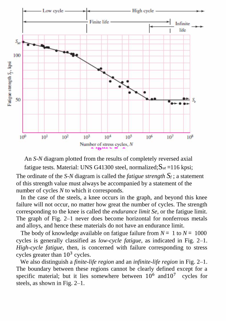
Figure 2–1

An S-N diagram plotted from the results of completely reversed axial

fatigue tests. Material: UNS G41300 steel, normalized;Sut =116 kpsi;

The ordinate of the S-N diagram is called the fatigue strength Sf ; a statement

of this strength value must always be accompanied by a statement of the

number of cycles N to which it corresponds. In the case of the steels, a knee occurs in the graph, and beyond this knee

failure will not occur, no matter how great the number of cycles. The strength

corresponding to the knee is called the endurance limit Se, or the fatigue limit.

The graph of Fig. 2–1 never does become horizontal for nonferrous metals

and alloys, and hence these materials do not have an endurance limit. The body of knowledge available on fatigue failure from N = 1 to N = 1000

cycles is generally classified as low-cycle fatigue, as indicated in Fig. 2–1.

High-cycle fatigue, then, is concerned with failure corresponding to stress

cycles greater than cycles. We also distinguish a finite-life region and an infinite-life region in Fig. 2–1.

The boundary between these regions cannot be clearly defined except for a

specific material; but it lies somewhere between and cycles for

steels, as shown in Fig. 2–1.

2–3 The Endurance Limit The determination of endurance limits by fatigue testing is now routine,

though a lengthy procedure. Generally, stress testing is preferred to strain

testing for endurance limits. There are great quantities of data in the literature on the results of rotating-

beam tests and simple tension tests of specimens taken from the same bar or

ingot. the endurance limit ranges from about 40 to 60 percent of the tensile

strength for steels up to about 210 kpsi (1450 MPa). For steels, the endurance

limit may be estimate as ………… (2-1)

where Sut is the minimum tensile strength. The prime mark on in this

equation refers to the rotating-beam specimen. When designs include detailed

heat-treating specifications to obtain specific microstructures, it is possible to

use an estimate of the endurance limit based on test data for the particular

microstructure; such estimates are much more reliable and indeed should be

used.

2–4 Endurance Limit Modifying Factors Joseph Marin, identified factors that quantified the effects of surface condition,

size, loading, temperature, and miscellaneous items. A Marin equation is

therefore written as

……………. (2-2)

where ka = surface condition modification factor

kb = size modification factor

kc = load modification factor

kd = temperature modification factor

ke = reliability factor

kf = miscellaneous-effects modification factor

= rotary-beam test specimen endurance limit

= endurance limit at the critical location of a machine

part in the geometry and condition of use.

When endurance tests of parts are not available, estimations are made by

applying Marin factors to the endurance limit.

Surface Factor ka:

The surface of a rotating-beam specimen is highly polished, The surface

modification factor depends on the quality of the finish of the actual part

surface and on the tensile strength of the part material. The data can be

represented by

……………… (2-3)

where Sut is the minimum tensile strength and a and b are to be found in

Table2–1.

EXAMPLE 2–1: A steel has a minimum ultimate strength of 520 MPa and a

machine surface Estimate ka.

Solution From Table 2–1, a = 4.51 and b =−0.265. Then, from Eq. (2–3)

ka = 4.51 = 0.860

Again, it is important to note that this is an approximation as the data is

typically quite scattered. Furthermore, this is not a correction to take lightly.

For example, if in the previous example the steel was forged, the correction

factor would be 0.540, a significant reduction of strength.

Size Factor kb: The size factor has been evaluated using 133 sets of data points. The

results for bending and torsion may be expressed as

……… (2-4)

the effective size of a round corresponding to a nonrotating solid or hollow

round. de = 0.370d ……… (2-5)

A rectangular section of dimensions h b, Using the same approach as before,

de = 0.808( …………. (2-6)

For axial loading there is no size effect, so

kb = 1 ……….. (2-7)

EXAMPLE 2–2 A steel shaft loaded in bending is 32 mm in diameter, abutting a filleted

shoulder 38 mm in diameter. The shaft material has a mean ultimate tensile

strength of 690 MPa. Estimate theMarin size factor kb if the shaft is used in

(a) A rotating mode.

(b) A nonrotating mode.

Solution: (a) From Eq. (2–4)

b) From Table 2–5,

From Eq. (2–4),

Loading Factor kc: When fatigue tests are carried out with rotating bending, axial (push-

pull), and torsional loading, the endurance limits differ with Sut. The

average values of the load factor as

…… (2-8)

Temperature Factor kd: When operating temperatures are below room temperature, brittle fracture is

a strong possibility and should be investigated first. When the operating

temperatures are higher than room temperature, yielding should be

investigated first because the yield strength drops off so rapidly with

temperature; see Fig. 2–2. Any stress will induce creep in a material

operating at high temperatures; so this factor must be considered too.

Finally, it may be true that there is no fatigue limit for materials operating

at high temperatures. Because of the reduced fatigue resistance, the failure

process is, to some extent, dependent on time.

Figure 2–2 A plot of the results of 145 tests of 21 carbon and alloy steels

showing the effect of operating temperature on the yield

strength Sy and the ultimate strength Sut . The ordinate is the

ratio of the strength at the operating temperature to the

strength at room temperature

Table 2–2 has been obtained from Fig. 2–2 by using only the tensile-strength

data. Note that the table represents 145 tests of 21 different carbon and alloy

steels. A fourthorder polynomial curve fit to the data underlying Fig. 2–2

gives …….. (2-9)

Where 70 ہ F Table 2–2

Effect of Operating Temperature on the Tensile Strength of

Steel.* (ST = tensile strength at operating temperature;

SRT = tensile strength at room temperature;

Two types of problems arise when temperature is a consideration. If the

rotating beam endurance limit is known at room temperature, then use

…………… (2-10)

from Table 2–2 or Eq. (2–9) and proceed as usual. If the rotating-beam

endurance limit is not given, then compute it using Eq. (2–1) and the

temperature-corrected tensile strength obtained by using the factor from

Table 2–2. Then use kd = 1.

EXAMPLE 2–3: A 1035 steel has a tensile strength of 70 kpsi and is to be used for a part

that sees 450°F in service. Estimate the Marin temperature modification

factor and (Se)450◦ if

(a) The room-temperature endurance limit by test is( 70◦= 39.0 kpsi.

(b) Only the tensile strength at room temperature is known.

Solution (a) First, from Eq. (2–9),

(b) Interpolating from Table 2–2 gives

Thus, the tensile strength at 450°F is estimated as

From Eq. (2–1) then,

Part a gives the better estimate due to actual testing of the particular material.

Reliability Factor ke:

The reliability modification factor can be determined from Table 2–3 as Table 2–3

Reliability Factors ke Corresponding to 8 Percent Standard

Deviation of the Endurance Limit

Miscellaneous-Effects Factor kf: Though the factor kf is intended to account for the reduction in endurance

limit due to all other effects, it is really intended as a reminder that these

must be accounted for, because actual values of kf are not always available. Residual stresses may either improve the endurance limit or affect it

adversely. Generally, if the residual stress in the surface of the part is

compression, the endurance limit is improved. Fatigue failures appear to be

tensile failures, or at least to be caused by tensile stress, and so anything that

reduces tensile stress will also reduce the possibility of a fatigue failure. Operations such as shot peening, hammering, and cold rolling build

compressive stresses into the surface of the part and improve the endurance

limit significantly. Of course, the material must not be worked to exhaustion. The endurance limits of parts that are made from rolled or drawn sheets or

bars, as well as parts that are forged, may be affected by the so-called

directional characteristics of the operation. Rolled or drawn parts, for

example, have an endurance limit in the transverse direction that may be 10

to 20 percent less than the endurance limit in the longitudinal direction.

Homework:

1. A in drill rod was heat-treated and ground. The measured hardness was

found to be 490 Brinell. Estimate the endurance strength if the rod is used in

rotating bending.

2. Estimate for the following materials:

(a) AISI 1020 CD steel.

(b) AISI 1080 HR steel.

(c) 2024 T3 aluminum.

(d) AISI 4340 steel heat-treated to a tensile strength of 250 kpsi.

3. Estimate the fatigue strength of a rotating-beam specimen made of

AISI 1020 hot-rolled steel corresponding to a life of 12.5 kilocycles of

stress reversal. Also, estimate the life of the specimen corresponding to a

stress amplitude of 36 kpsi. The known properties are Sut = 66.2 kpsi, σ0 =

115 kpsi, m = 0.22, and εf = 0.90.

4. Estimate the endurance strength of a 32-mm-diameter rod of AISI 1035

steel having a machined finish and heat-treated to a tensile strength of 710

MPa.

5. Bearing reactions R1 and R2 are exerted on the shaft shown in the figure,

which rotates at 1150 rev/min and supports a 10-kip bending force. Use a 1095

HR steel. Specify a diameter d using a design factor of nd =1.6 for a life of 3

min. The surfaces are machined.

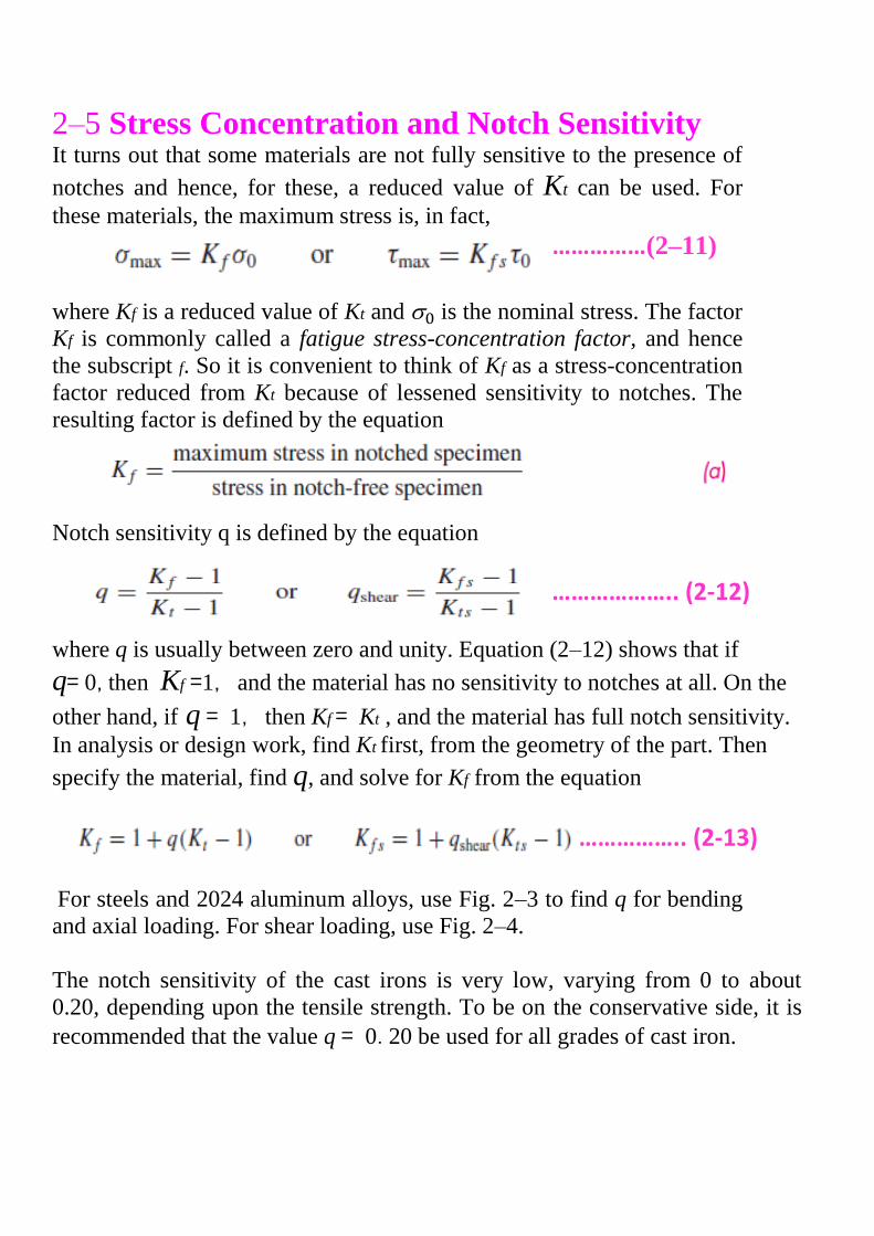
2–5 Stress Concentration and Notch Sensitivity It turns out that some materials are not fully sensitive to the presence of

notches and hence, for these, a reduced value of Kt can be used. For

these materials, the maximum stress is, in fact,

……………(2–11)

where Kf is a reduced value of Kt and is the nominal stress. The factor

Kf is commonly called a fatigue stress-concentration factor, and hence

the subscript f. So it is convenient to think of Kf as a stress-concentration

factor reduced from Kt because of lessened sensitivity to notches. The

resulting factor is defined by the equation Notch sensitivity q is defined by the equation

……………….. (2-12) where q is usually between zero and unity. Equation (2–12) shows that if q= 0,then Kf =1, and the material has no sensitivity to notches at all. On the

other hand, if q = 1, then Kf = Kt , and the material has full notch sensitivity.

In analysis or design work, find Kt first, from the geometry of the part. Then

specify the material, find q, and solve for Kf from the equation

…………….. (2-13) For steels and 2024 aluminum alloys, use Fig. 2–3 to find q for bending

and axial loading. For shear loading, use Fig. 2–4.

The notch sensitivity of the cast irons is very low, varying from 0 to about

0.20, depending upon the tensile strength. To be on the conservative side, it is

recommended that the value q = 0.20 be used for all grades of cast iron.

Figure 2–3 Notch-sensitivity charts for steels and UNS A92024-T wrought

aluminum alloys subjected to reversed bending or reversed axial

loads. For larger notch radii, use the values of q corresponding

to the r = 0.16-in (4-mm)

Figure 2–4

Notch-sensitivity curves for materials in reversed torsion.

For larger notch radii, use the values of q shear

corresponding to r = 0.16 in (4 mm).

EXAMPLE 2–4: A steel shaft in bending has an ultimate strength of 690 MPa and a shoulder

with a fillet radius of 3 mm connecting a 32-mm diameter with a 38-mm

diameter. Estimate Kf

Solution: From table.A-15 Fig. A–15–9, using D/d = 38/32 = 1.1875, r/d = 3/32 =

0.093 75, we read the graph to find Kt = 1.65.

From table.A-23, for Sut = 690 MPa = 100 kpsi, and r = 3 mm, and from

Fig. (2–3), obtain q = 0.84. Thus, from Eq. (2–13)

Answer Kf = 1 + q(Kt − 1)= 1 + 0.84(1.65 − 1) = 1.55

EXAMPLE 2–5: A 1015 hot-rolled steel bar has been machined to a diameter of 1 in. It is to be

placed in reversed axial loading for 70 000 cycles to failure in an operating

environment of 550°F. Using ASTM minimum properties, and a reliability of

99 percent, estimate the endurance limit.

Solution: From Table A–20, Sut =50 kpsi at 70°F. Since the rotating-

beam specimen endurance limit is not known at room temperature, we

determine the ultimate strength at the elevated temperature first, using

Table 2–2. From Table 2–2,

The ultimate strength at 550°F is then

The rotating-beam specimen endurance limit at 550°F is then estimated

from Eq. (2–1) as

Next, we determine the Marin factors. For the machined surface,

Eq. (2–3) with Table 2–1 gives

For axial loading, from Eq. (2–7), the size factor kb = 1, and from Eq. (2–8)

the loading factor is kc = 0.85. The temperature factor kd = 1, since we

accounted for the temperature in modifying the ultimate strength and

consequently the endurance limit. For 99 percent reliability, from Table 2–

3, ke = 0.814. Finally, since no other conditions were given, the

miscellaneous factor is kf = 1. The endurance limit for the part is estimated

by Eq. (2-2) as

Table.(A-20)

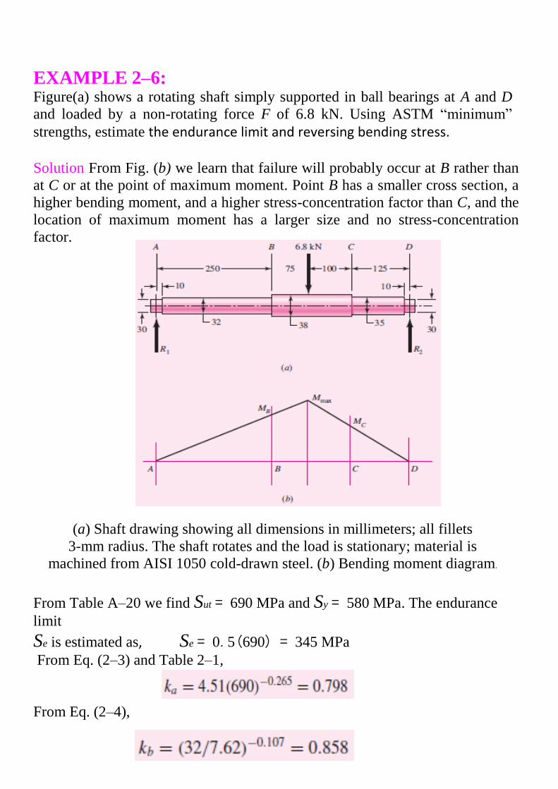
EXAMPLE 2–6: Figure(a) shows a rotating shaft simply supported in ball bearings at A and D

and loaded by a non-rotating force F of 6.8 kN. Using ASTM ―minimum‖

strengths, estimate the endurance limit and reversing bending stress. Solution From Fig. (b) we learn that failure will probably occur at B rather than

at C or at the point of maximum moment. Point B has a smaller cross section, a

higher bending moment, and a higher stress-concentration factor than C, and the

location of maximum moment has a larger size and no stress-concentration

factor.

(a) Shaft drawing showing all dimensions in millimeters; all fillets

3-mm radius. The shaft rotates and the load is stationary; material is

machined from AISI 1050 cold-drawn steel. (b) Bending moment diagram.

From Table A–20 we find Sut = 690 MPa and Sy = 580 MPa. The endurance

limit

Se is estimated as, Se = 0.5(690) = 345 MPa From Eq. (2–3) and Table 2–1,

From Eq. (2–4),

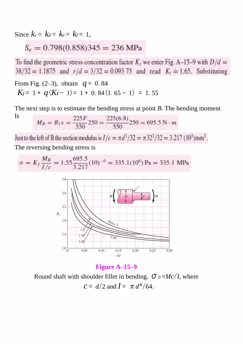
Since kc = kd = ke = kf = 1,

From Fig. (2–3), obtain q = 0.84

Kf = 1 + q(Kt − 1)= 1 + 0.84(1.65 − 1) = 1.55

The next step is to estimate the bending stress at point B. The bending moment

Is The reversing bending stress is

Figure A–15–9

Round shaft with shoulder fillet in bending. σ0 =Mc/I, where

c = d/2 and I = π /64.

2–6 Characterizing Fluctuating Stresses: Fluctuating stresses in machinery often take the form of a sinusoidal pattern

because of the nature of some rotating machinery. the shape of the wave is not

important, but the peaks on both the high side (maximum) and the low side

(minimum) are important. Thus Fmax and Fmin in a cycle of force can be used to

characterize the force pattern. then a steady component and an alternating component can be constructed

as follows:

where Fm is the midrange steady component of force, and Fa is the amplitude

of the alternating component of force.

Figure 2–5

The following relations are evident from Fig. 2–5: …………………… (2-14) The components of stress, some of which are shown in Fig. 6–23d, are

In addition to Eq. (6–36), the stress ratio …………………… (2-15) and the amplitude ratio ……………………. (2-16) are also defined and used in connection with fluctuating stresses.

. Equations (2–14) utilize symbols and as the stress components at

the location under scrutiny. This means, in the absence of a notch, and

are equal to the nominal stresses and induced by loads Fa

and Fm, respectively; in the presence of a notch they are Kf and

Kf , respectively, as long as the material remains without plastic strain.

In other words, the fatigue stress concentration factor Kf is applied to both

components.

2–7 Fatigue Failure Criteria for Fluctuating Stress Five criteria of failure are diagrammed in Fig. 2–6: the Soderberg, the modified

Goodman, the Gerber, the ASME-elliptic, and yielding. The diagram shows

that only the Soderberg criterion guards against any yielding, but is biased low. Considering the modified Goodman line as a criterion, point A represents a

limiting point with an alternating strength Sa and midrange strength Sm. The

slope of the load line shown is defined as r = Sa/Sm.

Figure 2–6

The criterion equation for the Soderberg line is …………………….. (2-17) Similarly, we find the modified Goodman relation to be …………………….. (2-18)

The Gerber failure criterion is written as ……………………… (2-19) and the ASME-elliptic is written as …………………….. (2-20) The Langer static yield ………………………. (2-21)

The stresses and can replace Sa and Sm, where n is the design

factor or factor of safety. Then, Eq. (2–17), the Soderberg line, becomes Soderberg ……………………… (2-22) mod-Goodman …………………….. (2-23) Gerber …………………….. (2-24) ASME-elliptic ……………………… (2-25) Langer static yield ………………….. (2-26)

the Gerber and ASME-elliptic for fatigue failure criterion and the Langer for

first-cycle yielding. However, conservative designers often use the modified

Goodman criterion,

The failure criteria are used in conjunction with a load line, r = Sa/Sm =

/ . Principal intersections are tabulated in Tables 2–4 to 2–6. Formal

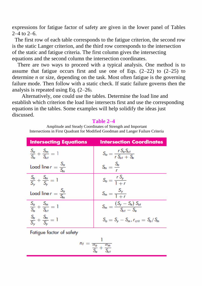
expressions for fatigue factor of safety are given in the lower panel of Tables

2–4 to 2–6. The first row of each table corresponds to the fatigue criterion, the second row

is the static Langer criterion, and the third row corresponds to the intersection

of the static and fatigue criteria. The first column gives the intersecting

equations and the second column the intersection coordinates. There are two ways to proceed with a typical analysis. One method is to

assume that fatigue occurs first and use one of Eqs. (2–22) to (2–25) to

determine n or size, depending on the task. Most often fatigue is the governing

failure mode. Then follow with a static check. If static failure governs then the

analysis is repeated using Eq. (2–26). Alternatively, one could use the tables. Determine the load line and

establish which criterion the load line intersects first and use the corresponding

equations in the tables. Some examples will help solidify the ideas just

discussed. Table 2–4

Amplitude and Steady Coordinates of Strength and Important

Intersections in First Quadrant for Modified Goodman and Langer Failure Criteria

Table 2–5 Amplitude and Steady Coordinates of Strength and Important

Intersections in First Quadrant for Gerber and Langer Failure

Criteria

Table 2–6 Amplitude and Steady Coordinates of Strength and Important

Intersections in First Quadrant for ASME -Elliptic and Langer

Failure Criteria

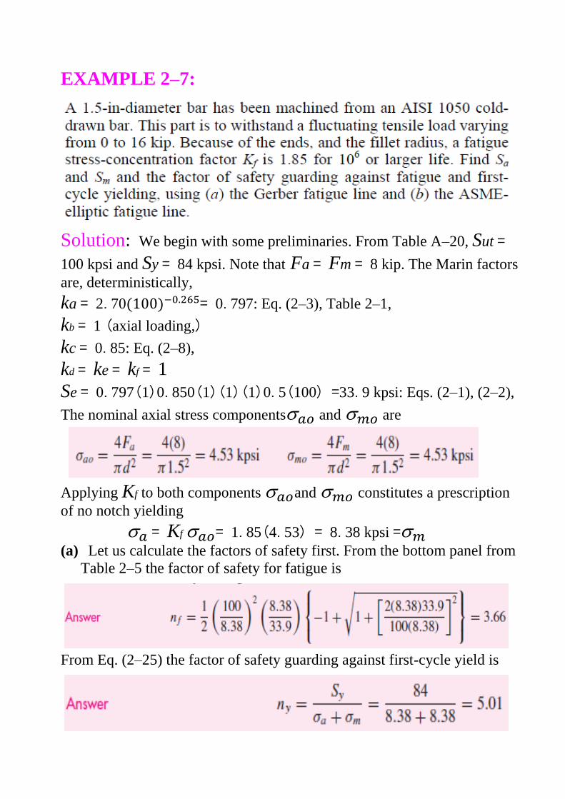
EXAMPLE 2–7:

Solution: We begin with some preliminaries. From Table A–20, Sut =

100 kpsi and Sy = 84 kpsi. Note that Fa = Fm = 8 kip. The Marin factors

are, deterministically,

ka = 2.70 = 0.797: Eq. (2–3), Table 2–1,

kb = 1 (axial loading,)

kc = 0.85: Eq. (2–8),

kd = ke = kf = 1

Se = 0.797(1)0.850(1)(1)(1)0.5(100) =33.9 kpsi: Eqs. (2–1), (2–2),

The nominal axial stress components and are

Applying Kf to both components and constitutes a prescription

of no notch yielding

= Kf = 1.85(4.53) = 8.38 kpsi = (a) Let us calculate the factors of safety first. From the bottom panel from

Table 2–5 the factor of safety for fatigue is From Eq. (2–25) the factor of safety guarding against first-cycle yield is

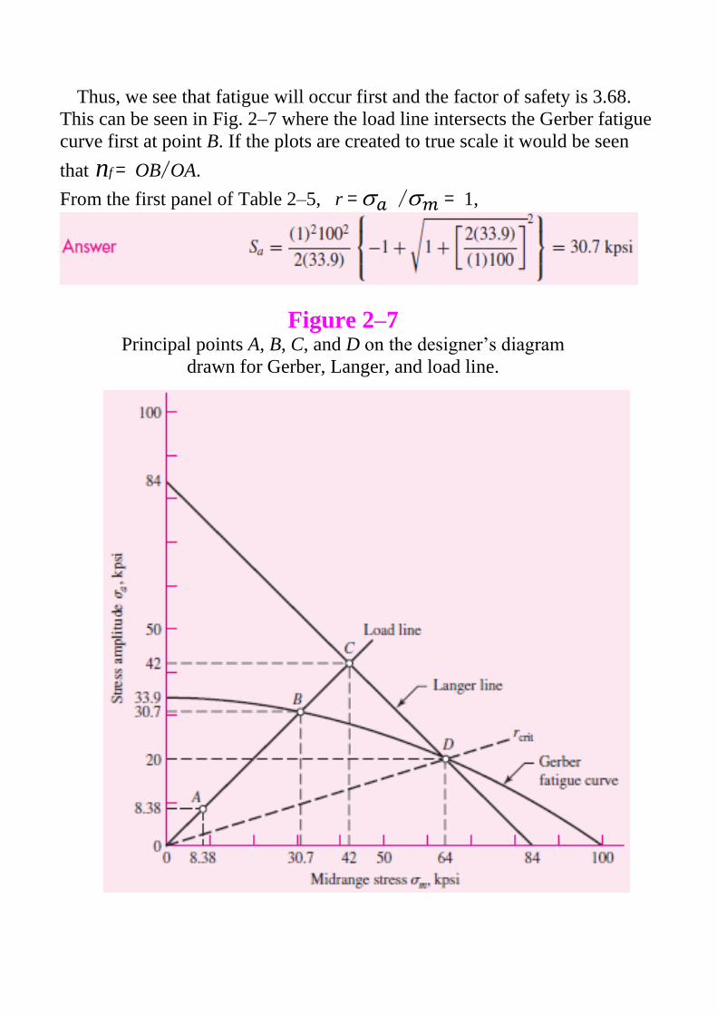
Thus, we see that fatigue will occur first and the factor of safety is 3.68.

This can be seen in Fig. 2–7 where the load line intersects the Gerber fatigue

curve first at point B. If the plots are created to true scale it would be seen

that nf = OB/OA.

From the first panel of Table 2–5, r = / = 1,

Figure 2–7 Principal points A, B, C, and D on the designer’s diagram

drawn for Gerber, Langer, and load line.

We could have detected that fatigue failure would occur first without

drawing Fig.2 –7 by calculating . From the third row third column

panel of Table 2–5, the intersection point between fatigue and first-cycle

yield is The critical slope is thus

which is less than the actual load line of r = 1. This indicates that fatigue

occurs before first-cycle-yield.

(b) Repeating the same procedure for the ASME-elliptic line, for fatigue

Again, this is less than ny =5.01 and fatigue is predicted to occur first.

From the first row second column panel of Table 2–6, with r =1, we

obtain the coordinates Sa and Sm of point B in Fig. 2–8 as

To verify the fatigue factor of safety, nf = Sa/ = 31.4/8.38 = 3.75.

Figure 2–8 Principal points A, B, C, and D on the designer’s diagram

drawn for ASME-elliptic, Langer, and load lines.

As before, let us calculate . From the third row second column panel

of Table 2–6,

which again is less than r = 1, verifying that fatigue occurs first with

nf = 3.75.

For many brittle materials, the first quadrant fatigue failure criteria

follows a concave upward Smith-Dolan locus represented by

…………. (2-27)

or as a design equation,

………….. (2-28)

For a radial load line of slope r, we substitute Sa/r for Sm in Eq. (2–27)

and solve for Sa , obtaining

…………. (2-29)

The most likely domain of designer use is in the range from −Sut ≤ ≤

Sut . The locus in the first quadrant is Goodman, Smith-Dolan, or

something in between. The portion of the second quadrant that is used is

represented by a straight line between the points −Sut , Sut and 0, Se,

which has the equation

………… (2-30)

EXAMPLE2–8: A grade 30 gray cast iron is subjected to a load F applied to a 1 by

-in

cross-section link with a

-in-diameter hole drilled in the center as

depicted in Fig. 2–9a. The surfaces are machined. In the neighborhood of

the hole, what is the factor of safety guarding against failure under the

following conditions:

(a) The load F = 1000 lbf tensile, steady.

(b) The load is 1000 lbf repeatedly applied.

(c) The load fluctuates between −1000 lbf and 300 lbf without column

action. Use the Smith-Dolan fatigue locus.

Figure 2–9

The grade 30 cast-iron part in axial fatigue with (a) its geometry

displayed and (b) its designer’s fatigue diagram for the

circumstances of Ex. 2–8.

0.25/1 = 0.25, and Kt = 2.45. The notch sensitivity for cast iron is

0.20 (it is recommended that the value q = 0.20 be used for all grades of

cast iron.). so

From Eq. (2–29), From Eq. (2–30),

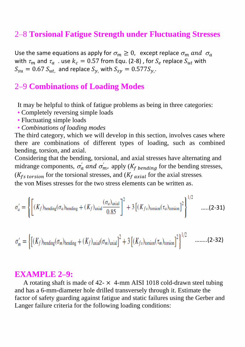
2–8 Torsional Fatigue Strength under Fluctuating Stresses Use the same equations as apply for except replace with and . use from Equ. (2-8) , for replace with and replace with .

2–9 Combinations of Loading Modes It may be helpful to think of fatigue problems as being in three categories:

• Completely reversing simple loads

• Fluctuating simple loads

• Combinations of loading modes The third category, which we will develop in this section, involves cases where

there are combinations of different types of loading, such as combined

bending, torsion, and axial. Considering that the bending, torsional, and axial stresses have alternating and

midrange components,

apply ( for the bending stresses,

( for the torsional stresses, and ( for the axial stresses.

the von Mises stresses for the two stress elements can be written as. …..(2-31) ……..(2-32)

EXAMPLE 2–9: A rotating shaft is made of 42- 4-mm AISI 1018 cold-drawn steel tubing

and has a 6-mm-diameter hole drilled transversely through it. Estimate the

factor of safety guarding against fatigue and static failures using the Gerber and

Langer failure criteria for the following loading conditions:

(a) The shaft is subjected to a completely reversed torque of 120 N .m in

phase with a completely reversed bending moment of 150 N.m.

(b) The shaft is subjected to a pulsating torque fluctuating from 20 to 160

N .m and a steady bending moment of 150 N .m.

Solution : Here we follow the procedure of estimating the strengths and

then the stresses, followed by relating the two.

From Table A–20 we find the minimum strengths to be Sut = 440 MPa and Sy

= 370 MPa. The endurance limit of the rotating-beam specimen is

0.5(440) = 220 MPa. The surface factor, obtained from Eq. (2–3) and Table 2–

1, is From Eq. (2–4) the size factor is The remaining Marin factors are all unity, so the modified endurance strength

Se is

(a) Theoretical stress-concentration factors are found from Table A–16. Using a/D = 6/42 = 0.143 and d/D = 34/42 = 0.810, and using

linear interpolation, we obtain A = 0.798 and Kt = 2.366 for bending;

and A = 0.89 and Kts = 1.75 for torsion. Thus, for bending, and for torsion Next, using Figs. 2–3 and 2–4,with a notch radius of 3 mm we find the notch

sensitivities to be 0.78 for bending and 0.96 for torsion. The two corresponding

fatigue stress-concentration factors are obtained from Eq. (2–13) as.

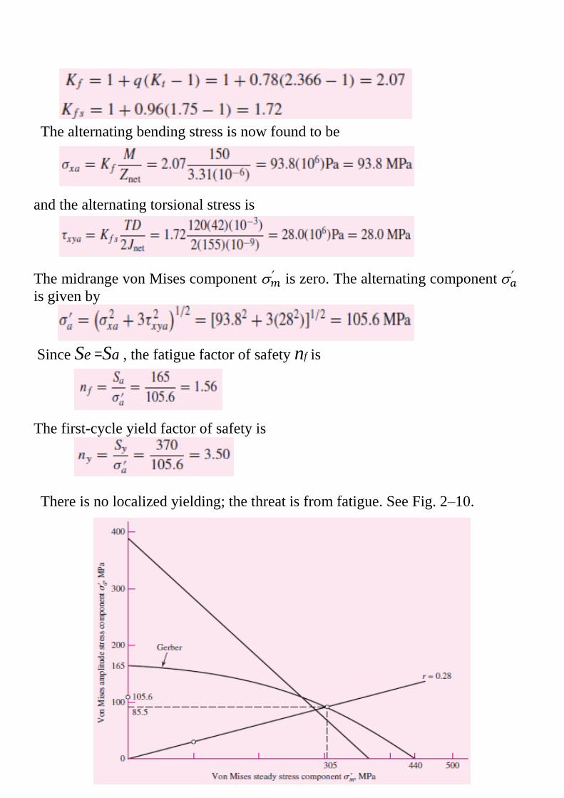
The alternating bending stress is now found to be and the alternating torsional stress is The midrange von Mises component

is zero. The alternating component

is given by

Since Se =Sa , the fatigue factor of safety nf is The first-cycle yield factor of safety is There is no localized yielding; the threat is from fatigue. See Fig. 2–10.

Figure 2–10

Designer’s fatigue diagram for Ex. 2–9.

(b) This part asks us to find the factors of safety when the alternating component is due

(b) This part asks us to find the factors of safety when the alternating

component is due to pulsating torsion, and a steady component is due to both

torsion and bending. We have

Ta = (160 − 20)/2 = 70 N .m and Tm = (160 + 20)/2 = 90 N .m

Corresponding amplitude and steady-stress components are

The steady bending stress component xm is

The von Mises components and

are From Table 2–5, the fatigue factor of safety is

From the same table, with r =

= 28.2/100.6 = 0.280, the strengths can be

shown to be Sa = 85.5 MPa and Sm = 305 MPa. See the plot in Fig. 2–10.

The first-cycle yield factor of safety ny is There is no notch yielding. The likelihood of failure may first come from first-

cycle yielding at the notch. See the plot in Fig. 2–9.

Homework: 1. A bar of steel has the minimum properties Se = 276 MPa, Sy = 413 MPa,

and Sut = 551 MPa. The bar is subjected to a steady torsional stress of 103

MPa and an alternating bending stress of 172 MPa. Find the factor of safety

guarding against a static failure, and either the factor of safety guarding

against a fatigue failure or the expected life of the part. For the fatigue

analysis use:

(a) Modified Goodman criterion.

(b) Gerber criterion.

(c) ASME-elliptic criterion.

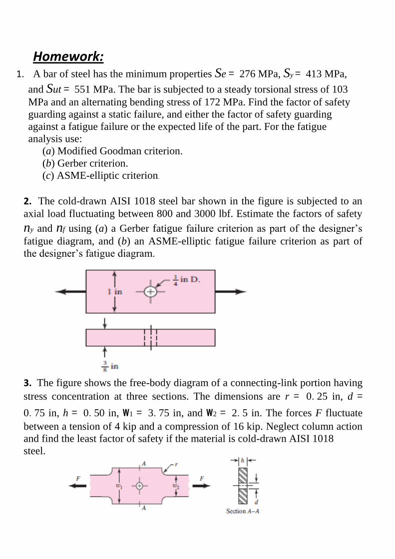
2. The cold-drawn AISI 1018 steel bar shown in the figure is subjected to an

axial load fluctuating between 800 and 3000 lbf. Estimate the factors of safety

ny and nf using (a) a Gerber fatigue failure criterion as part of the designer’s

fatigue diagram, and (b) an ASME-elliptic fatigue failure criterion as part of

the designer’s fatigue diagram. 3. The figure shows the free-body diagram of a connecting-link portion having

stress concentration at three sections. The dimensions are r = 0.25 in, d =

0.75 in, h = 0.50 in, w1 = 3.75 in, and w2 = 2.5 in. The forces F fluctuate

between a tension of 4 kip and a compression of 16 kip. Neglect column action

and find the least factor of safety if the material is cold-drawn AISI 1018

steel.

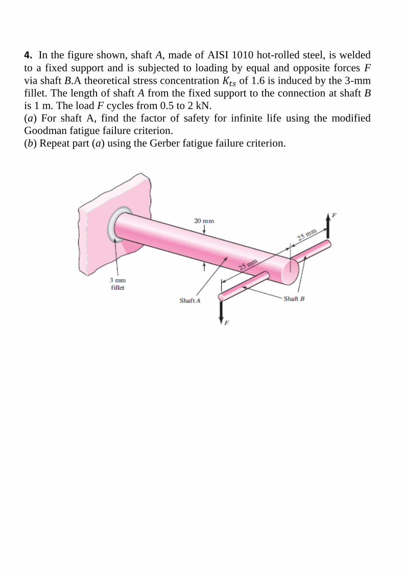
4. In the figure shown, shaft A, made of AISI 1010 hot-rolled steel, is welded

to a fixed support and is subjected to loading by equal and opposite forces F

via shaft B.A theoretical stress concentration of 1.6 is induced by the 3-mm

fillet. The length of shaft A from the fixed support to the connection at shaft B

is 1 m. The load F cycles from 0.5 to 2 kN.

(a) For shaft A, find the factor of safety for infinite life using the modified

Goodman fatigue failure criterion.

(b) Repeat part (a) using the Gerber fatigue failure criterion.