ENGINEERING GUIDELINES FOR THE EVALUATION OF HYDROPOWER … · engineering guidelines for the...
100
ENGINEERING GUIDELINES FOR THE EVALUATION OF HYDROPOWER PROJECTS CHAPTER 13 – EVALUATION OF EARTHQUAKE GROUND MOTIONS MAY 30, 2018 FEDERAL ENERGY REGULATORY COMMISSION 888 First Street, NC Washington, DC 20426
Transcript of ENGINEERING GUIDELINES FOR THE EVALUATION OF HYDROPOWER … · engineering guidelines for the...

ENGINEERING GUIDELINES FOR THE EVALUATION OF HYDROPOWER
PROJECTS
CHAPTER 13 – EVALUATION OF EARTHQUAKE GROUND MOTIONS
MAY 30, 2018 FEDERAL ENERGY REGULATORY COMMISSION
888 First Street, NC Washington, DC 20426

EVALUATION OF EARTHQUAKE GROUND MOTIONS
Prepared by
I. M. Idriss, Professor Emeritus, Univ. of California at Davis Consulting Geotechnical Engineer, Santa Fe, NM
e-mail: [email protected]
Ralph J. Archuleta, Professor Emeritus Department of Earth Science & Earth Research Institute
University of California at Santa Barbara e-mail: [email protected]
and Norman A. Abrahamson
Consulting Engineering Seismologist, Piedmont, CA e-mail: [email protected] & [email protected]
Prepared for
Division of Dam Safety and Inspections Office of Energy Projects
Federal Energy Regulatory Commission (FERC) 888 First Street, N.E.
Washington, D.C. 20426
May 30, 2018

Evaluation of Earthquake Ground Motions Page i May 30, 2018 For The Federal Energy Regulatory Commission (FERC) by I. M. Idriss, R. J. Archuleta and N. A. Abrahamson
TABLE OF CONTENTS Page 1.0 INTRODUCTION 1 1.1 Introductory Comments 1 1.2 Organization of the Report 2 2.0 EARTHQUAKE HAZARDS AND CONSEQUENCES
2
2.1 General
2
2.2 Fault Rupture
2
2.3 Soil Failure
5
2.4 Seiches 11 3.0 GEOLOGIC AND SEISMOLOGIC CONSIDERATIONS
12
3.1 Historical Seismicity
12
3.2 Seismographic Record
12
3.3 Geologic Studies
13
3.4 Earthquake Recurrence Models
22
3.5 Other Seismic Sources 27 4.0 SEISMIC HAZARD EVALUATION
28
4.1 Deterministic Seismic Hazard Evaluation
28
4.2 Probabilistic Seismic Hazard Evaluation
30
5.0 ESTIMATION OF EARTHQUAKE GROUND MOTIONS AT A ROCK OUTCROP
32
5.1 General
32
5.2 Empirical Procedures
33
5.3 Analytical Procedures 33 6.0 GUIDELINES
34
6.1 Required Geologic Studies
34

Evaluation of Earthquake Ground Motions Page ii May 30, 2018 For The Federal Energy Regulatory Commission (FERC) by I. M. Idriss, R. J. Archuleta and N. A. Abrahamson
6.2 Required Seismologic Studies
34
6.3 Deterministic Development of Earthquake Ground Motions
35
6.4 Probabilistic Development of Earthquake Ground Motions
35
6.5 Minimum Required Parameters for Controlling Events(s)
36
7.0 REFERENCES 37 APPENDIX A: METHODS FOR ESTIMATING MAXIMUM EARTHQUAKE MAGNITUDE
APPENDIX B: SELECTION OF APPROPRIATE PERCENTILE GROUND MOTION LEVEL IN A DETERMINISTIC SEISMIC HAZARD EVALUATION
APPENDIX C: EXAMPLES – PROBABILISTIC SEISMIC HAZARD ANALYSIS
APPENDIX D: EARTHQUAKE GROUND MOTIONS MODELS
APPENDIX E: ANALYTICAL SIMULATIONS TO GENERATE ACCELEROGRAMS AT A ROCK SITE
APPENDIX F: SELECTION OF ACCELEROGRAMS FOR SEISMIC ANALYSIS

Evaluation of Earthquake Ground Motions Page iii May 30, 2018 For The Federal Energy Regulatory Commission (FERC) by I. M. Idriss, R. J. Archuleta and N. A. Abrahamson
LIST OF TABLES Table 1 Examples of Slip Rates
LIST OF FIGURES Figure 2-1 Horizontal (Strike-Slip) Fault Offset of the Imperial Fault in 1940 across the All-
America Canal Caused by the 1940 El Centro Earthquake
Figure 2-2 Red Canyon Fault Scarp East of Blarney Stone Ranch Caused by the 1959Montana Earthquake
Figure 2-3 Fault Rupture of San Fernando Fault in 1971; the late Professor H. Bolton Seedwas Standing on the Hanging Wall and Lloyd Cluff was Standing on the Footwall(Photograph: Courtesy of Professor Clarence Allen)
Figure 2-4 View of Dam in Taiwan Prior to the Occurrence of the 1999 Chi Chi Earthquake
Figure 2-5 View of Dam after the 1999 Chi-Chi Earthquake Showing Damage to Portion ofDam due to Fault Rupture
Figure 2-6 View of fault rupture adjacent to bridge downstream of the dam, shown in Figures 2-4 and 2-5, resulting in formation of falls in river and damage to bridge structure.
Figure 2-7 Aerial View of Austrian Dam
Figure 2-8 Longitudinal and Transverse Cracks in Austrian Dam Caused by Shaking duringthe 1989 Loma Prieta Earthquake (after Vrymoed & Lam, 1991)
Figure 2-9 Vertical and Horizontal Displacements, in feet, of the Crest of Austrian Dam atStation 6+00 (after Vrymoed & Lam, 1991)
Figure 2-10 Vertical and Horizontal Displacements, in feet, of the Crest of Austrian Dam at Station 2+50 (after Vrymoed & Lam, 1991)
Figure 2-12 San Fernando Dam Complex shortly after the Occurrence of the 1971 SanFernando Earthquake
Figure 2-13 View of Upper San Fernando Dam Showing Horizontal and Vertical Deformationsand Cracks in the Upstream Face of the Dam
Figure 2-14 Close-up View of Cracks in the Upstream Face of Upper San Fernando Dam
Figure 2-15 Aerial View Lower San Fernando Dam before the occurrence of the 1971 SanFernando Earthquake showing the Extensive Number of Residences that WouldHave Been Affected by a Breach of the Dam (Photograph: Courtesy of DavidGutierrez)
Figure 2-16 Photograph of the Lower San Fernando Dam taken a few Hours after theOccurrence of the 1971 San Fernando Earthquake

Evaluation of Earthquake Ground Motions Page iv May 30, 2018 For The Federal Energy Regulatory Commission (FERC) by I. M. Idriss, R. J. Archuleta and N. A. Abrahamson
Figure 2-17 Photograph of the Lower San Fernando Dam taken after Partial Emptying the
Reservoir Showing the Extent of Lateral Flow of the Upstream Shell and Crest ofthe Dam
Figure 2-18 View of the Madison River Slide from Earthquake Lake Side; Slide occurred during the 1959 Montana Earthquake
Figure 3-1 Aerial View of San Andreas Fault near Palmdale Reservoir in Southern California (From Richter, 1958)
Figure 3-2 Log of Trench across Fault on which the 1968 Borrego Mountain, California, Earthquake Occurred (From Clark et al., 1972)
Figure 3-3 Schematic Illustration of Four Types of Faults
Figure 3-4 Relation between Moment Magnitude and Various Magnitude Scales (after Heaton et al., 1982)
Figure 3-5 Relationship between M and bLgm
Figure 3-6 Location Map of the South-Central Segment of the San Andreas Fault
Figure 3-7 Plot of Instrumental Seismicity Data for the Period of 1900 – 1980 Along the
South-Central Segment of the San Andreas Fault; the Box in the Figure Represents Range of Recurrence for M = 7.5 – 8, Based on Geologic Data (from Schwartz and Coppersmith, 1984)
Figure 3-8 Characteristic Earthquake Recurrence Model for South Central Segment of San Andreas Fault

Evaluation of Earthquake Ground Motions Page 1 May 30, 2018 For The Federal Energy Regulatory Commission (FERC) by I. M. Idriss, R. J. Archuleta and N. A. Abrahamson
EVALUATION OF EARTHQUAKE GROUND MOTIONS
by
I. M. Idriss, Ralph J. Archuleta and Norman A. Abrahamson 1.0 INTRODUCTION 1.1 Introductory Comments The Division of Dam Safety and Inspections of the Office of Energy Projects at the Federal Energy Regulatory Commission (FERC) is responsible for the safety of power-generating stations throughout the USA. This responsibility includes concern with the effects of earthquakes at these stations, which typically include dams and appurtenant structures. Accordingly, FERC requested that the writers prepare this document on "Evaluation of Earthquake Ground Motions" that contains the main elements that could be utilized by FERC to establish "Seismic Design Criteria" for all facilities under its jurisdiction. The purpose of seismic design criteria is to provide guidelines and procedures for obtaining earthquake ground motion parameters for use in evaluating the seismic response of a given structure or facility. Presently, there are three ways by which the earthquake ground motion parameters can be ascertained: (i) use of local building codes; (ii) conducting a deterministic seismic hazard analysis (DSHA); and (iii) conducting a probabilistic seismic hazard analysis (PSHA). Typically, local building codes are intended to mitigate collapse of buildings and loss of life, and do not apply to structures covered in this document. Both deterministic and probabilistic seismic hazard analyses and evaluations are covered in this document. The earthquake ground motion parameters discussed in this document pertain to a "rock outcrop". Thus, these parameters are intended for use as input to an analytical model that would include the structure under consideration, e.g., a dam-foundation system. Any effects of local site conditions on earthquake ground motions would then be explicitly accounted for in the analyses. Accordingly, the effects of local site conditions on earthquake ground motions, which can be very significant, are not addressed in this document. To provide the needed basis for estimating earthquake ground motion parameters at a particular "rock outcrop", it is necessary to incorporate the appropriate geologic and seismologic input and to utilize the most relevant available procedures for estimating these parameters. The remaining pages of this document cover these aspects and the appendices include more details regarding specific aspects of the seismic hazard evaluation procedures.

Evaluation of Earthquake Ground Motions Page 2 May 30, 2018 For The Federal Energy Regulatory Commission (FERC) by I. M. Idriss, R. J. Archuleta and N. A. Abrahamson
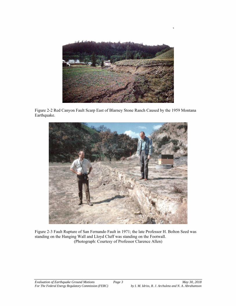
1.2 Organization of the Report In addition to this introductory section, the report includes six sections and six appendices and a list of references. The appendices are structured so that they can be updated periodically as new developments and publications pertinent to each appendix become available. 2.0 EARTHQUAKE HAZARDS AND CONSEQUENCES 2.1 General This section is included in this document merely to highlight why seismic hazards can be very important to facilities under the jurisdiction of FERC. Hazards that may affect such facilities include fault rupture, soil failure, and seiches. Other hazards, such as tsunamis, are not discussed in this document because all of the facilities under FERC's jurisdiction are inland and are unlikely to be affected by tsunamis. 2.2 Fault Rupture Fault rupture is a hazard that must be dealt with whenever a fault traverses a dam site. The potential for the presence of a fault, or fault traces, at a particular site should be fully investigated to assess the location, orientation, type, sense of movement … etc. Typical examples of fault rupturing in historic earthquakes are presented in Figures 2-1 through 2-6. Possible approaches to allowing for the effects of fault rupture on embankment dams are offered, for example, in Sherard et al. (1974) and other regulatory documents. The exact method that the licensee uses must be appropriately documented.
Figure 2-1 Horizontal (Strike-Slip) fault offset of the Imperial Fault in 1940 across the All-America Canal caused by the 1940 El Centro earthquake.
Evaluation of Earthquake Ground Motions Page 3 May 30, 2018 For The Federal Energy Regulatory Commission (FERC) by I. M. Idriss, R. J. Archuleta and N. A. Abrahamson
Figure 2-2 Red Canyon Fault Scarp East of Blarney Stone Ranch Caused by the 1959 Montana Earthquake.
Figure 2-3 Fault Rupture of San Fernando Fault in 1971; the late Professor H. Bolton Seed was standing on the Hanging Wall and Lloyd Cluff was standing on the Footwall.
(Photograph: Courtesy of Professor Clarence Allen)

Evaluation of Earthquake Ground Motions Page 4 May 30, 2018 For The Federal Energy Regulatory Commission (FERC) by I. M. Idriss, R. J. Archuleta and N. A. Abrahamson
Figure 2-4 View of dam in Taiwan prior to the occurrence of the 1999 Chi-Chi earthquake.
Figure 2-5 View of dam after the 1999 Chi-Chi Earthquake showing damage to portion of the dam due to fault rupture.

Evaluation of Earthquake Ground Motions Page 5 May 30, 2018 For The Federal Energy Regulatory Commission (FERC) by I. M. Idriss, R. J. Archuleta and N. A. Abrahamson
Figure 2-6 View of fault rupture adjacent to bridge downstream of the dam, shown in Figures 2-4 and 2-5, resulting in formation of falls in river and damage to bridge structure.
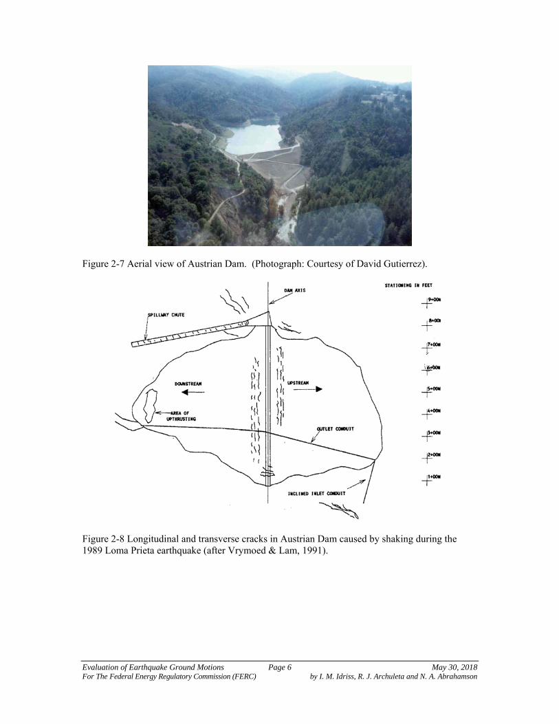
2.3 Soil Failure 2.3.1 Foundation and/or Embankment Soils Strong earthquake ground motions can induce high pore water pressures and/or high strains in these soils that could have serious consequences, including:
Settlements, which are mostly abrupt and non-uniform and often lead to longitudinal as well as transverse cracks.
Loss of bearing support. Floatation of buried structures, such as underground tanks or pipes. Increased lateral pressures against retaining structures. Lateral spreads (limited lateral movements). Lateral flows (extensive lateral movements).
Examples of settlements leading to cracks coupled with limited lateral movements are illustrated by the performance of Austrian Dam in California during the 1989 Loma Prieta earthquake as shown in Figures 2-7 through 2-10.
Evaluation of Earthquake Ground Motions Page 6 May 30, 2018 For The Federal Energy Regulatory Commission (FERC) by I. M. Idriss, R. J. Archuleta and N. A. Abrahamson
Figure 2-7 Aerial view of Austrian Dam. (Photograph: Courtesy of David Gutierrez).
Figure 2-8 Longitudinal and transverse cracks in Austrian Dam caused by shaking during the 1989 Loma Prieta earthquake (after Vrymoed & Lam, 1991).

Evaluation of Earthquake Ground Motions Page 7 May 30, 2018 For The Federal Energy Regulatory Commission (FERC) by I. M. Idriss, R. J. Archuleta and N. A. Abrahamson
Figure 2-9 Vertical and horizontal displacements, in feet, of the crest of Austrian Dam at Station 6+00 (after Vrymoed & Lam, 1991).
Figure 2-10 Vertical and horizontal Displacements, in feet, of the crest of Austrian Dam at Station 2+50 (after Vrymoed & Lam, 1991).
Among the consequences of increased pore water pressure is the possibility of triggering liquefaction in cohesionless soils, such as sands, silty sands and very low plasticity or non-plastic sandy silt. An example of liquefaction "in progress" is shown in Figure 2-11 – a view captured during the magnitude 7½ 1978 Miyagi-Ken-Oki earthquake in Japan.
Figure 2-11 Surface evidence of liquefaction triggered during the 1978 Miyagi-Ken-Oki earthquake in Japan.

Evaluation of Earthquake Ground Motions Page 8 May 30, 2018 For The Federal Energy Regulatory Commission (FERC) by I. M. Idriss, R. J. Archuleta and N. A. Abrahamson
Examples of lateral spreads (limited lateral movements) and lateral flows (extensive lateral movements) are provided by what happened to the Upper and Lower San Fernando Dams during the 1971 San Fernando earthquake, as shown in Figure 2-12. Figures 2-13 and 2-14 provide more details of the relatively limited lateral movements (lateral spreads) of the embankment of the Upper San Fernando Dam.
Figure 2-12 San Fernando Dam Complex shortly after the occurrence of the 1971 San Fernando earthquake.
Figure 2-13 View of Upper San Fernando Dam showing horizontal and vertical deformations and cracks in the upstream face of the dam.
UPPER DAM
LOWER DAM

Evaluation of Earthquake Ground Motions Page 9 May 30, 2018 For The Federal Energy Regulatory Commission (FERC) by I. M. Idriss, R. J. Archuleta and N. A. Abrahamson
Figure 2-14 Close-up View of Cracks in the Upstream Face of Upper San Fernando Dam.
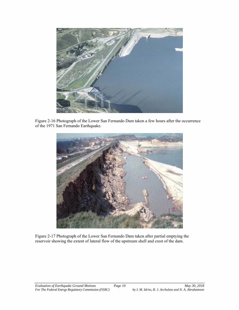
An aerial view of the Lower San Fernando Dam before the occurrence of the 1971 San Fernando earthquake is shown in Figure 2-15. The devastating effects of the earthquake on this dam are presented in Figures 2-16 and 2-17. Note that the lateral flows caused by the ground shaking were initiated because of the liquefaction of the soils in the upstream shell of the dam and the resulting loss of strength of these soils.
Figure 2-15 Aerial view Lower San Fernando Dam before the occurrence of the 1971 San Fernando Earthquake showing the extensive number of residences that would have been affected by a breach of the dam (Photograph: Courtesy of David Gutierrez).
Evaluation of Earthquake Ground Motions Page 10 May 30, 2018 For The Federal Energy Regulatory Commission (FERC) by I. M. Idriss, R. J. Archuleta and N. A. Abrahamson
Figure 2-16 Photograph of the Lower San Fernando Dam taken a few hours after the occurrence of the 1971 San Fernando Earthquake.
Figure 2-17 Photograph of the Lower San Fernando Dam taken after partial emptying the reservoir showing the extent of lateral flow of the upstream shell and crest of the dam.

Evaluation of Earthquake Ground Motions Page 11 May 30, 2018 For The Federal Energy Regulatory Commission (FERC) by I. M. Idriss, R. J. Archuleta and N. A. Abrahamson
2.3.2 Reservoir Rim Landslides along the rim of the reservoir can be triggered by the ground shaking during an earthquake. Such landslides could impact the body of dam negatively, e.g., blocking an intake tower, generating a wave that may overtop the crest etc. An example of a landslide is the Madison River Slide in the 1959 Montana earthquake shown in Figure 2-18.
Figure 2-18 View of the Madison River Slide from earthquake lake side; Slide occurred during the 1959 Montana Earthquake. (from USGS 1964)
2.4 Seiches A seiche is a standing wave in an enclosed or partly enclosed body of water. Seiches are normally caused by earthquake activity, and can affect reservoirs, harbors, bays, lakes, rivers and canals. In the majority of instances, earthquake-induced seiches do not occur close to the source of an earthquake, but some distance away (possibly as far as 100s of kilometers). This is due to the fact that earthquake seismic waves close to the source are richer in high frequencies, while those at greater distances are of lower frequency content which can enhance the rhythmic movement in a body of water. The biggest seiches develop when the period of the ground shaking matches the period of oscillation of the water body. In 1891, an earthquake near Port Angeles caused an eight-foot seiche in Lake Washington; such a rise in reservoir level could result in overtopping if the free board is not sufficient at the time. The 1964 Alaska earthquake created seiches on 14 inland bodies of water in the state of Washington, including Lake Union where several pleasure craft, houseboats and floats sustained some damage. Inland areas, though not vulnerable to tsunamis, are vulnerable to seiches caused by earthquakes. Additional vulnerabilities include water storage tanks, and containers of liquid hazardous materials that are also affected by the rhythmic motion.

Evaluation of Earthquake Ground Motions Page 12 May 30, 2018 For The Federal Energy Regulatory Commission (FERC) by I. M. Idriss, R. J. Archuleta and N. A. Abrahamson
Seiches create a "sloshing" effect on bodies of water and liquids in containers. This primary effect can cause damage to moored boats, piers and facilities close to the water. Secondary problems, including landslides and floods, are related to accelerated water movements and elevated water levels. The above description was obtained from text available from the following web site: https://earthquake.usgs.gov/learn/topics/seiche.php 3.0 GEOLOGIC AND SEISMOLOGIC CONSIDERATIONS Earthquake ground motions at a particular site are estimated through a seismic hazard evaluation. The geologic and seismologic inputs needed for completing a seismic hazard evaluation consist of acquiring information regarding the following key elements:
a. The seismic sources on which future earthquakes are likely to occur;
b. The size of the possible earthquakes and the frequency with which an earthquake is likely to occur on each source; and
c. The distance and orientation of each source with respect to the site.
This information is obtained from the following sources of data in the region in which the site is located: (1) The historical seismicity record; (2) the seismographic, or instrumental, record of earthquake activity in the region; and (3) the geologic history, especially within the past few thousand to several hundred thousand years. 3.1 Historical Seismicity A necessary first step in a seismic hazard evaluation is the compilation and documentation of the historical seismicity record pertinent to the region in which the site is located. It is essential in assessing this historical seismicity record that local sources of data (e.g., newspaper accounts, manuscripts written about a specific earthquake, etc.) be critically reviewed and that conflicting information be resolved. The historical seismicity record in the USA is relatively brief as it extends only over the past 200 to 400 years. It may be noted, however, that a good deal of the available historical records for many parts of the country have been compiled and can be accessed. It is also important to note that much of the historic seismicity record relies heavily (if not exclusively) on reports of felt ground motions or patterns of damage. Important as the historical seismicity record is, however, it is not sufficient by itself to estimate the future seismic activity in a region. 3.2 Seismographic Record The seismographic, or instrumental, record in a region is also an important tool in a seismic hazard evaluation. Instrumental records augment the historical records by providing quantitative data (e.g., size, location, depth, mechanism, and time of occurrence of earthquakes) that are not available from reports of felt ground motions or patterns of damage. The seismographic record is available only since the year 1900 and, until recently, only from a limited number of stations in selected areas worldwide. Significant increases in the number of
Evaluation of Earthquake Ground Motions Page 13 May 30, 2018 For The Federal Energy Regulatory Commission (FERC) by I. M. Idriss, R. J. Archuleta and N. A. Abrahamson
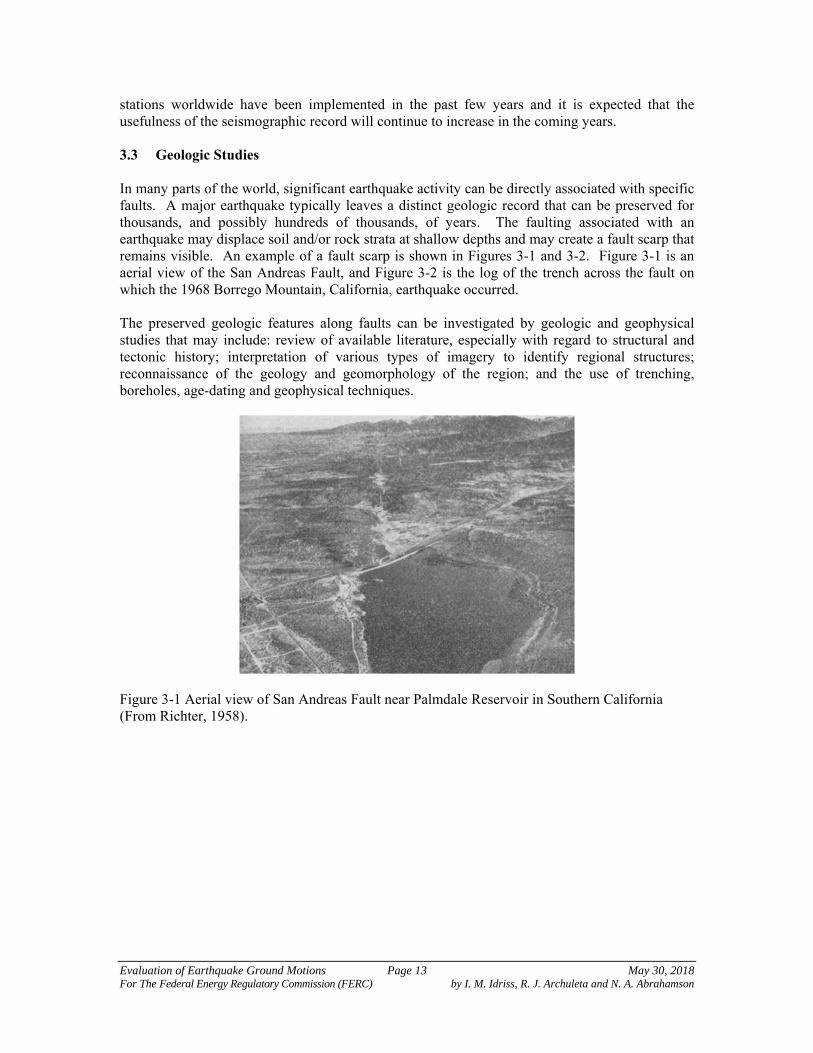
stations worldwide have been implemented in the past few years and it is expected that the usefulness of the seismographic record will continue to increase in the coming years. 3.3 Geologic Studies In many parts of the world, significant earthquake activity can be directly associated with specific faults. A major earthquake typically leaves a distinct geologic record that can be preserved for thousands, and possibly hundreds of thousands, of years. The faulting associated with an earthquake may displace soil and/or rock strata at shallow depths and may create a fault scarp that remains visible. An example of a fault scarp is shown in Figures 3-1 and 3-2. Figure 3-1 is an aerial view of the San Andreas Fault, and Figure 3-2 is the log of the trench across the fault on which the 1968 Borrego Mountain, California, earthquake occurred. The preserved geologic features along faults can be investigated by geologic and geophysical studies that may include: review of available literature, especially with regard to structural and tectonic history; interpretation of various types of imagery to identify regional structures; reconnaissance of the geology and geomorphology of the region; and the use of trenching, boreholes, age-dating and geophysical techniques.
Figure 3-1 Aerial view of San Andreas Fault near Palmdale Reservoir in Southern California (From Richter, 1958).

Evaluation of Earthquake Ground Motions Page 14 May 30, 2018 For The Federal Energy Regulatory Commission (FERC) by I. M. Idriss, R. J. Archuleta and N. A. Abrahamson
Figure 3-2 Log of Trench across fault on which the 1968 Borrego Mountain, California, earthquake occurred (From Clark et al., 1972).
There are various types of faults, as shown in Figure 3-3. In a thrust (or a reverse) fault, the offset is along an inclined plane and occurs in response to a compressive tectonic strain environment as shown in Figure 3-3a; examples of major earthquakes on such faults are the 1952 Kern County and the 1971 San Fernando earthquakes in California, and the 1999 Chi-Chi earthquake in Taiwan. The offset on a normal fault is also along an inclined plane, but it occurs in response to extensional strain (Figure 3-3b); examples are the 1954 Dixie Valley, Nevada, and the 1959 Hebgen Lake, Montana, earthquakes. Offset along a strike slip fault is essentially lateral and occurs along a vertical, or near-vertical, plane as illustrated in Figure 3-3c; examples are the 1906 San Francisco earthquake in Northern California and the 1992 Landers earthquake in Southern California. The types of faults illustrated in Figures 3-3a, 3-3b and 3-3c are designated as crustal faults and the illustrations presented in the figure indicate that rupture had extended to the ground surface. Earthquakes have also occurred on crustal faults on which rupture did not extend to the ground surface; these faults are designated as "blind". Examples of earthquakes occurring on "blind" faults are the 1983 Coalinga, the 1987 Whittier-Narrows, and the 1994 Northridge earthquakes in California. The mechanism of each of these earthquakes was a thrust mechanism and the fault involved is designated as a "blind thrust" (Stein and Yeats 1989) Subduction zones (Figure 3-3d) occur at the interface between tectonic plates. Examples of earthquakes occurring in subduction zones are the magnitude 9.2 Alaska earthquake in 1964, the magnitude 9.5 Chilean earthquake in 1960, the magnitude 8.1 Michoacán, Mexico, and numerous earthquakes in Japan such the magnitude 8.3 Hokkaido earthquake off the eastern shore of Hokkaido in 2003, and the magnitude 9.1 Tohoku earthquake off the eastern shore of Japan in 2011.

Evaluation of Earthquake Ground Motions Page 15 May 30, 2018 For The Federal Energy Regulatory Commission (FERC) by I. M. Idriss, R. J. Archuleta and N. A. Abrahamson
a. Thrust faulting under
horizontal compressive strains b. Normal faulting resulting
from extensional strains
c. Strike-slip displacement on a vertical fault plane
d. Under thrust faulting in a subduction zone
Figure 3-3 Schematic illustration of four types of faults.
Over the years, geologists and seismologists have studied the detailed characteristics of faults, and, until recently, designated each as being a potentially active fault or an inactive fault. This designation is based on recency of fault displacement, which leads to rigid legal definitions of fault activity based on a specified time criterion. Typically, the more critical the facility, the longer is the time criterion specified. For example, the US Nuclear Regulatory Commission considers, for nuclear plants, a fault active if it shows evidence of multiple displacements in the past 500,000 years, or evidence of a single displacement in the past 35,000 years. For dams, the US Bureau of Reclamation specifies 100,000 years, and the US Army Corps of Engineers uses 35,000 years. Faults that have had displacements within these time spans are considered active and those that have not had displacements are considered inactive. Classifying faults as either "active" or "inactive" does not provide sufficient information about the nature of the fault. Instead, geologists and seismologists have recognized that significant differences exist in the degrees of activity of various faults. These differences are manifested by several key fault parameters, which are briefly described below. 3.3.1 Key Fault Parameters The key fault parameters that appear most significant include: rate of strain release, or fault slip rate; amount of fault displacement in each event; length (and area) of fault rupture; earthquake size; and earthquake recurrence interval. Slip Rate: The geologic slip rate provides a measure of the average rate of deformation on a fault. The slip rate is estimated by dividing the amount of cumulative displacement, measured from displaced geologic or geomorphic features, by the estimated age of the geological material or feature. The geologic slip rate is an average value over a geologic time period, and reliable to the

Evaluation of Earthquake Ground Motions Page 16 May 30, 2018 For The Federal Energy Regulatory Commission (FERC) by I. M. Idriss, R. J. Archuleta and N. A. Abrahamson
extent that strain accumulation and release over this time period has been uniform and responding to the same tectonic stress environment. Examples of ranges of slip rates of a few well-known faults are listed in Table 1.
Table 1 – Examples of slip rates on a number of well-known faults Fault Slip Rate (mm/year)
Fairweather, Alaska 38 to 74 San Andreas, California 20 to 53
Hayward Fault, Northern California 7 to 11 Wasatch, Utah 0.9 to 1.8
Newport-Inglewood, Southern California
0.1 to 1.2
Atlantic Coast faults 0.0002 The information in Table 1 leads to the following observations: (i) prominent and highly active faults, such as the San Andreas Fault, have a much higher slip rate than minor faults; and (ii) uncertainties exist regarding the slip rate and a range of values needs to be considered in specific application. Observation (ii) pertains to various segments of the fault as well as to a specific segment of the fault. Slip Per Event: The amount of fault displacement for each fault rupture event differs among faults and fault segments and provides another indication of relative differences in degrees of fault activity. The differences in displacement are influenced by the tectonic environment, fault type and geometry, pattern of faulting, and the amount of accumulated strain released. The amount of slip per event can be directly measured in the field during studies of historical faulting and is usually reported in terms of a maximum and an average value for the entire fault or for segments of the fault. Displacements for prehistoric rupture events can be estimated for some faults from detailed surface and subsurface seismic geologic investigations (e.g., Sieh, 1978; Swan et al., 1980). It is often difficult to ascertain what value of maximum or average displacement is most accurate and representative from data available in the literature. Often, reported displacements represent apparent displacement or separation across a fault. For normal faulting events, scarp height has typically been reported as a measurement of the tectonic displacement. The scarp height, however, often exceeds the net tectonic displacement across a fault by as much as two times, due to graben formation and other effects near the fault (Swan et al., 1980). In the case of thrust faults, the reported vertical displacement often is actually the measure of vertical separation, and the net slip on the fault can be underestimated by a significant amount (e.g., Cluff and Cluff, 1984). Thus, it is very important that the database, from which displacements are determined, be carefully evaluated before selecting the best estimate of maximum or average displacement from data available in the literature. Fault Area: The fault area is critical for both deterministic and probabilistic methods that are used to estimate the earthquake ground motions. The geometry of the fault controls the distance between the fault and the site and is used in estimating the magnitude (seismic moment) of the maximum earthquake.

Evaluation of Earthquake Ground Motions Page 17 May 30, 2018 For The Federal Energy Regulatory Commission (FERC) by I. M. Idriss, R. J. Archuleta and N. A. Abrahamson
Earthquake Size: The earliest measures of earthquake size were based on the maximum intensity and areal extent of perceptible ground shaking (most of the non-instrumental historical seismicity record is expressed in terms of these two observations). Instrumental recordings of ground shaking led to the development of the magnitude scale (Richter, 1935). The magnitude was intended to represent a measure of the energy released by the earthquake, independent of the place of observation. As stated by Richter (1958): "Magnitude was originally defined as the logarithm of the maximum amplitude on a seismogram written by an instrument of specific standard type at a distance of 100 km. … Tables were constructed empirically to deduce from any given distance to 100 km. … The zero of the scale is fixed arbitrarily to fit the smallest recorded earthquakes." Mathematically, the magnitude is expressed as follows:
10 10 oMagnitude M Log A Log A [1]
in which A is the recorded trace amplitude for a given earthquake at a given distance as written by the standard type of instrument, and Ao is the amplitude for a particular earthquake selected as standard. For local earthquakes, A and Ao are measured in millimeters and the standard instrument is the Wood-Anderson torsion seismograph which has a natural period of 0.8 sec, a damping factor of 0.8 (i.e., 80 percent of critical) and static magnification of 2800. A magnitude determined in this way is designated the local magnitude, ML. For purposes of determining magnitudes for teleseisms, Gutenberg and Richter (1956) devised the surface wave magnitude, MS, and the body wave magnitudes, mb and mB. The local magnitude is determined at a period of 0.8 sec, the body wave magnitudes are determined at periods between 1 and 5 sec, and the surface wave magnitude is determined at a period of 20 sec. In the past 30 or so years, the use of seismic moment, Mo, has provided a physically more meaningful measure of the size of a faulting event. Seismic moment, with units of force times length (dyne-cm or N-m) is expressed by the equation:
o fM A D [2]
in which µ is the shear modulus of the material along the fault plane and is typically equal to 3×10¹¹ dyne/cm2 for crustal rocks, Af is the area, in square centimeters, of the fault plane undergoing slip, and D, in cm, is the average slip over the surface of the fault that had non-zero slip. Seismic moment provides a basic link between the physical parameters that characterize the faulting and the seismic waves radiated due to rupturing along the fault. Seismic moment is, therefore, a more useful measure of the size of an earthquake. Kanamori (1977) and Hanks and Kanamori (1979) introduced a moment-magnitude scale, M M , in which magnitude is calculated from seismic moment using the following formula:
10 1.5 16.05oLog M M
or
102 3 16.05oM Log M [3]

Evaluation of Earthquake Ground Motions Page 18 May 30, 2018 For The Federal Energy Regulatory Commission (FERC) by I. M. Idriss, R. J. Archuleta and N. A. Abrahamson
where seismic moment is given in dyne-cm. The moment magnitude is different from other magnitude scales because it is directly related to average slip and ruptured fault area, while the other magnitude scales reflect the amplitude of a particular type of seismic wave. The relationships between moment magnitude and the other magnitude scales, shown in Figure 3-4, were presented by Heaton et al. (1982) based on both empirical and theoretical considerations as well as previous work by others. The following observations can be made from the results shown in Figure 3-4:
1. Except for moment magnitude, all magnitude scales exhibit a limiting value, or a saturation level, with increasing moment magnitude. Saturation appears to occur when the ruptured fault dimension becomes much larger than the wave length of seismic waves that are used in measuring the magnitude. Moment magnitude does not saturate because it is derived from seismic moment as opposed to an amplitude on a seismogram.
2. The local magnitude, ML, and the short-period body wave magnitude, mb, are essentially equal to moment magnitude up to M = 6.
3. The long period body-wave magnitude, mB, is essentially equal to moment magnitude up to M = 7.5.
4. The surface wave magnitude, MS, is essentially equal to moment magnitude in the range of M = 6 to 8.
Moment Magnitude, M
2 3 4 5 6 7 8 9 10
Mag
nit
ud
e
2
3
4
5
6
7
8
9
mb
ML
MS
mB
MSM L
Magnitude Scale
ML - Local
MS - Surface Wave
mb - Short-Period Body Wave
mB - Long-Period Body Wave
Figure 3-4 Relation between Moment Magnitude and Various Magnitude Scales (after Heaton et al., 1982) Typically, the size of an earthquake is reported in terms of local magnitude, surface wave magnitude, or body wave magnitude, or in terms of all these magnitude scales. Based on the observations made from Figure 3-4, the use of local magnitude for magnitudes smaller than 6, and surface wave magnitude for magnitudes greater than 6 but less than 8 is equivalent to using the moment magnitude. For great earthquakes, such as the 1960 Chilean earthquake (M = 9.5) and the

Evaluation of Earthquake Ground Motions Page 19 May 30, 2018 For The Federal Energy Regulatory Commission (FERC) by I. M. Idriss, R. J. Archuleta and N. A. Abrahamson
1964 Alaska earthquake (M = 9.2), however, it is important to use the moment magnitude to express the size of the earthquake. In fact, it is best to use the moment magnitude scale for all events. It should be noted that the magnitude derived using Eq. [3] is defined as the moment magnitude and given the designation M. This moment magnitude is devised in a way that it is equivalent to ML for 3 < ML < 6. Another, slightly different magnitude is the energy magnitude, MW, which is given by the following relationship (Kanamori, 1977):
10 1.5 16.1o WLog M M
or
102 3 16.1W oM Log M [4]
The magnitudes M and MW are nearly equal and have been used interchangeably in many applications. The magnitude scale most often used for central and eastern US earthquakes is mbLg, which was developed by Nuttli (1973). It is based on measuring the maximum amplitude, in microns, of 1-sec period Lg waves and was devised to be equivalent to mb. Nuttli initially called this magnitude mb. To avoid confusion with the true mb, however, this magnitude is usually referred to as mbLg. It is also called Nuttli magnitude and designated mN (Atkinson and Boore, 1987); it is referred to as such in the Canadian network. Boore and Atkinson (1987) derived the following relationship between Nuttli's magnitude and moment magnitude:
22.689 0.252 0.127N NM m m [4]
Frankel et al. (1996) also derived a relationship between moment magnitude and mbLg, namely:
22.45 0.473 0.145bLg bLgM m m [5]
Equations [4] and [5] provide nearly identical values of moment magnitude, M, for the same values of mbLg as illustrated in Figure 3-5.

Evaluation of Earthquake Ground Motions Page 20 May 30, 2018 For The Federal Energy Regulatory Commission (FERC) by I. M. Idriss, R. J. Archuleta and N. A. Abrahamson
Magnitude mbLg
4 5 6 7 8 9
Mo
men
t M
agn
itu
de,
M
4
5
6
7
8
9
Atkinson & Boore (1987)
Frankel et al (1996)
Figure 3-5 Relationship between M and mbLg The use of magnitude or seismic moment as a criterion for the comparison of fault activity requires the choice of the magnitude or moment value that is characteristic of the fault. In many instances, it is not possible to ascertain whether historical seismic activity is characteristic of the fault through geologic time, unless evidence of the sizes of past earthquakes is available from seismic geology studies of paleo seismicity. As noted earlier, even a long historical seismic record is not enough by itself (Allen, 1976). In a few cases, detailed seismic geology studies have provided data on the sizes of past surface faulting earthquakes (e.g., Sieh, 1978). In general, these data involve measurements of prehistoric rupture length and/or displacement, and a derived magnitude can be estimated probably within one-half magnitude. Methods for Estimating Maximum Earthquake Magnitude: There are several available methods for assigning a maximum earthquake magnitude to a given fault (e.g., Wyss, 1979; Slemmons, 1982; Schwartz et al., 1984; Wells and Coppersmith, 1994). These methods are based on empirical correlations between magnitude and some key fault parameter such as: fault rupture length and surface fault displacement measured following surface faulting earthquakes; and fault length and width estimated from studies of aftershock sequences. Data from worldwide earthquakes have been used in regression analyses of magnitude on length, magnitude on displacement, and magnitude on rupture area. In addition, magnitude can be calculated from seismic moment and a relationship between magnitude and slip rate has also been proposed. Each method has some limitations, which may include: non-uniformity in the quality of the empirical data, a somewhat limited data set, and a possible inconsistent grouping of data from different tectonic environments. A number of these methods are summarized in Appendix A. Geological and seismological studies can define fault length, fault width, amount of displacement per event, and slip rate for potential earthquake sources. These data provide estimates of maximum magnitude on each source. Selection of a maximum magnitude for each source is ultimately a judgment that incorporates understanding of specific fault characteristics, the regional tectonic environment, similarity to other faults in the region, and data on regional seismicity.

Evaluation of Earthquake Ground Motions Page 21 May 30, 2018 For The Federal Energy Regulatory Commission (FERC) by I. M. Idriss, R. J. Archuleta and N. A. Abrahamson
Use of a number of magnitude estimation methods can result in more reliable estimates of maximum magnitude than the use of any one single method. In this way, a wide range of fault parameters can be included and the selected maximum magnitude will be the estimate substantiated by the best available data. To evaluate the possible range of maximum magnitude estimates for a source, uncertainties in the fault parameters and in the magnitude relationships need to be identified and evaluated. Recurrence Interval of Significant Earthquakes: Faults having different degrees of activity differ significantly in the average recurrence intervals of significant earthquakes. Comparisons of recurrence provide a useful means of assessing the relative activity of faults, because the recurrence interval provides a direct link between slip rate and earthquake size. Recurrence intervals can be calculated directly from slip-rate, as discussed later in this report, and displacement-per-event data. In some cases, where the record of instrumental seismicity and/or historical seismicity is sufficiently long compared to the average recurrence interval, seismicity data can be incorporated when estimating recurrence. In, many regions of the world, however, the instrumental as well as the historical seismicity record is too brief; some active faults have little or no historical seismicity and the recurrence time between significant earthquakes is longer than the available historical record along the fault of interest. Plots of frequency of occurrence versus magnitude can be prepared for small to moderate earthquakes and extrapolations to larger magnitudes can provide estimates of the mean rate of occurrence of larger magnitude earthquakes. This technique has limitations, however, because it is based on regional seismicity, and often cannot result in reliable recurrence intervals for specific faults. The impact of such extrapolation on hazard evaluations is discussed in the following section. 3.4 Earthquake Recurrence Models A key element in a seismic hazard evaluation is estimating recurrence intervals for various magnitude earthquakes. A general equation that describes earthquake recurrence may be expressed as follows:
,N m f m t [6]
in which N(m) is the number of earthquakes with magnitude greater than or equal to m, and t is time. The simplest form of Eq. [6] that has been used in most applications is the well-known Richter's law of magnitudes (Gutenberg and Richter, 1956; Richter, 1958) which states that the occurrence of earthquakes during a given period of time can be approximated by the relationship:
10Log N m a bm [7]
in which 10a is the total number of earthquakes with magnitude greater than zero and b is the slope. This equation assumes spatial and temporal independence of all earthquakes, i.e., it has the properties of a Poisson Model. For engineering applications, the recurrence is limited to a range of magnitudes between mo and mu. The magnitude mo is the smallest magnitude of concern in the specific application; in most cases mo can be limited to magnitude 5 because little or no damage has occurred from earthquakes with magnitudes less than 5. The magnitude mu is the largest magnitude the fault is considered capable of producing; the value of mu depends on the geologic and seismologic considerations summarized earlier. The cumulative distribution is then given by:

Evaluation of Earthquake Ground Motions Page 22 May 30, 2018 For The Federal Energy Regulatory Commission (FERC) by I. M. Idriss, R. J. Archuleta and N. A. Abrahamson
|
o uM
o
o u
F m P M m m m m
N m N m
N m N m
[8]
The probability density function is equal to:
M M
df m F m
dm [9]
In Equations [6] through [9], the letters m or M refer to magnitude; the upper case denotes a random variable, and the lower case denotes a specific value of magnitude. When the recurrence relationship is expressed by Richter's law of magnitudes, the following expression is obtained by substituting Eq. [7] into Eq. [8]:
1 10
11 10
o
u o
b m m
o
b m mN m A
[10]
The parameter Ao is the number of events for earthquakes with magnitude greater than or equal to mo (i.e., Log10 (Ao) = a - bmo). Development of Equation [10] requires knowledge of the parameters Ao, b and mu, and a selection of mo. The parameter Ao and slope b are based on either the historical seismicity record (including the instrumental record when available) or on geologic data. The slope b, based on regional historical seismicity records, typically ranges from 0.6 to about 1.1. For most faults, the historical seismicity record is relatively short and most of the information is for smaller magnitudes (typically less than 6). Thus, for these smaller magnitude earthquakes, a reasonable fit using Richter's relationship can be obtained and values of Ao and b can be calculated. Discrepancies between earthquake recurrence intervals based on historical seismicity and recurrence intervals based on geologic data are common when applied to a specific fault. A good example of such a discrepancy is found for the south-central segment of the San Andreas fault, whose location is shown in Figure 3-6. Schwartz and Coppersmith (1984) compiled the historical instrumental seismicity for the period 1900-1980 along this segment of the fault. Using these data, they developed the recurrence curve shown in Figure 3-7, which is represented by the equation: Log10(N(m)) = 3.30 – 0.88m. The instrumental historical seismicity data available for this fault include earthquakes only up to magnitude 6±. Also shown in Figure 3-7 is a box that represents the estimate of recurrence for the magnitude range of 7.5 to 8 based on geologic data (Sieh, 1978). As can be noted from the plots in Figure 3-7, if the line developed from historical seismicity is extrapolated to the magnitude range of 7.5 to 8, the recurrence for such magnitude earthquakes would be underestimated by a factor of about 15 compared to the recurrence estimated from geologic data.

Evaluation of Earthquake Ground Motions Page 23 May 30, 2018 For The Federal Energy Regulatory Commission (FERC) by I. M. Idriss, R. J. Archuleta and N. A. Abrahamson
Figure 3-6 Location of the South-Central Segment of the San Andreas Fault.
Magnitude, m
3 4 5 6 7 8 9
An
nu
al N
um
ber
of
Ear
thq
uak
es w
ith
Mag
nit
ud
e m
0.0001
0.001
0.01
0.1
1
10
1900 - 1932
1932 - 1980
1857 aftershocks
Log N(m) = 3.36 - 0.88m
Figure 3-7 Plot of instrumental seismicity data from 1900 to 1980 along the south-central segment of the San Andreas Fault; the box in the figure represents range of recurrence for M = 7.5 – 8, based on geologic data (from Schwartz and Coppersmith, 1984).

Evaluation of Earthquake Ground Motions Page 24 May 30, 2018 For The Federal Energy Regulatory Commission (FERC) by I. M. Idriss, R. J. Archuleta and N. A. Abrahamson
Molnar (1979) developed a procedure to calculate recurrences based on geologic slip rate and seismic moment (Eq. 2). The seismic moment rate, or the rate of energy release along a fault, as estimated by Brune (1968) is given by:
T
o fM A S
[11]
And by Molnar (1979):
u
o
Tm
o omM n m M m dm
[12]
In which S is the average slip rate in cm/year and n m dN m dm . Differentiating Eq. [10],
substituting into Eq. [12], integrating and equating the results to Eq. [11] provides the following:
1 fo
u oo o
k A Sc bA
b kM M
[13]
In which 10 1.5 16.05, and u oo o oLog M M M M are the seismic moments corresponding to
mu and mo, respectively, and 10u ob m m
k
. Equation [13] is also derived on the premise that slip takes place on the fault not only because of the occurrence of mu, but also during earthquakes with smaller magnitudes, i.e., the strain accumulated along the fault is released through slip due to the occurrence of all magnitude earthquakes. Wesnousky et al. (1983) suggest, based on data from Japan, that the accumulated strain on a fault is periodically released in earthquakes of only the maximum magnitude, mu. Wesnousky et al. formulated a recurrence model based on this premise, which they designate as the maximum magnitude recurrence model. The recurrence interval, Tu in years, for the maximum magnitude is the ratio of the seismic moment (Eq. 3) associated with the maximum magnitude divided by the seismic moment rate (Eq. 11); thus:
101.5 16.05 /u ufT Log m A S
1u uN m T
[14]
Earthquakes with magnitude ranging from mo to (mu – X), which constitute foreshocks and aftershocks to the maximum earthquake, are assumed to obey Richter’s recurrence model with a slope equal to the regional b. The value of X is typically equal to 1 to 1.5. Note that since the occurrence of earthquakes with less than or equal to (mu – X) is conditional on the occurrence of mu, it follows that N(mu – X) = N(mu). Another model, which has been used in many applications, is the characteristic earthquake recurrence model (Schwartz and Coppersmith, 1984). This model uses Eq. [7] for the magnitude range mo to an intermediate magnitude with a slope based on historical or instrumental seismicity. The recurrence of the maximum magnitude, mu, is evaluated from geologic data using Eq. [14]. The recurrence between the intermediate magnitude and the maximum magnitude using a relation similar to Eq. [7] but having a slope much smaller than the slope used for the magnitude range mo to the intermediate magnitude, as illustrated in Figure 3-8.

Evaluation of Earthquake Ground Motions Page 25 May 30, 2018 For The Federal Energy Regulatory Commission (FERC) by I. M. Idriss, R. J. Archuleta and N. A. Abrahamson
The characteristic recurrence model for the south-central segment of the San Andreas fault is shown in Figure 3-8.
Magnitude, m
4 5 6 7 8 9
An
nu
al N
um
ber
of
Ear
thq
uak
es w
ith
Mag
nit
ud
e m
0.001
0.01
0.1
1
Log10 (N(m)) = -0.42 - 0.25m
Log10 (N(m)) = 3.36 - 0.88m
Historical Data Range ofGeologic
Data1900 - 1932
1932 - 1980
1857 aftershocks
Figure 3-8 Characteristic earthquake recurrence model for south central-segment of San Andreas Fault. This is a plot of the number of earthquakes per year with a magnitude greater than or equal to the magnitude plotted on the abscissa. For example, there is one earthquake every 10 years with a magnitude greater than or equal M = 5.

Evaluation of Earthquake Ground Motions Page 26 May 30, 2018 For The Federal Energy Regulatory Commission (FERC) by I. M. Idriss, R. J. Archuleta and N. A. Abrahamson
3.5 Other Seismic Sources The sources described in the previous sections consist of specific faults or fault zones. In many parts of the world there are no known or suspected faults and hence seismic activity in those parts cannot be associated with any specific fault or fault zone. In these cases, earthquakes are considered to occur in a "seismic zone" extending over an area that is typically identified based on felt area and/or instrumental seismicity during past earthquakes. This approach is usually used in Eastern North America (ENA). Even in geologic settings with a number of known faults, an areal source centered on the site is also considered as a possible seismic source. Often this source is assigned to account for instrumental seismicity that cannot be associated with any known (or suspected) fault. Such a seismic source is usually described as a "background zone" or a "random" source. Background seismic zones have been assigned in many parts of Western North America (WNA) such as Washington, Oregon and California. The distance from the site to such areal seismic sources is usually assigned as a "depth" below the site and typically varies from 5 to 15 km. Data from instrumental seismicity (which would include the depth of each event) are necessary for assigning this depth. The maximum moment magnitude considered for such zones is typically M = 6½ ± ¼. 4.0 SEISMIC HAZARD EVALUATION The purpose of a seismic hazard evaluation is to arrive at earthquake ground motion parameters for use in evaluating the site and facilities during seismic loading conditions. Coupled with the vulnerability of the site and the facilities under various levels of these ground motion parameters, the risk to which the site and the facilities may be subject to can be assessed. Alternate designs, modifications, etc. can then be considered. As noted earlier, there are three ways by which the earthquake ground motion parameters are obtained, namely: use of local building codes; conducting a deterministic seismic hazard evaluation; or conducting a probabilistic seismic hazard evaluation. Local building codes contain a seismic zone map that includes minimum required seismic design parameters. Typically, local building codes are intended to mitigate collapse of buildings and loss of life, and do not apply to structures covered in this document. 4.1 Deterministic Seismic Hazard Analysis (DSHA) In a deterministic analysis and evaluation, the current practice consists of the following steps:
a. A geologic and seismologic evaluation is conducted to define the sources (faults and /or seismic zones) relevant to the site;
b. The maximum magnitude, mu, on each source is estimated (Appendix A) and the
appropriate distance to the site is determined; c. Recurrence relationships for each source are derived using historical seismicity as well as
geologic data and an earthquake with a magnitude 2um m is selected for each source
such that the recurrence N(m2) for 2m m is the same for all sources; if, for example,

Evaluation of Earthquake Ground Motions Page 27 May 30, 2018 For The Federal Energy Regulatory Commission (FERC) by I. M. Idriss, R. J. Archuleta and N. A. Abrahamson
N(m2) = 0.005 per year (i.e., a recurrence of 200 years) is used, this earthquake is then designated the "200-year" earthquake;
d. The needed earthquake ground motion parameters (e.g., accelerations, velocities, spectral
ordinates, etc.) are calculated, using one or more attenuation relationship, or an analytical procedure, for the maximum earthquake, mu, and for m2 from each source; and
e. The magnitude and distance producing the largest ground motion parameter for um and for m2 are then used for analysis and design purposes.
Note that the earthquake having the maximum magnitude (Step b) has often been designated the "maximum credible earthquake" or MCE. For critical structures, usually the MCE is used for selecting the earthquake ground motions. Attenuation relationships (earthquake ground motion models, or GMMs), such as those discussed in Section 5.0 below and in Appendix D, are used to obtain the values of these motions. Typically, the median values obtained from these attenuation relationships are used when the seismic source has a relatively low degree of activity. For high slip rate sources, the 84th-percentile values are used, as discussed in summarized below and described in more detail in Appendix B. Appendix B provides an approach for assessing the average slip rate below which the median values can be used and the average slip rate above which the 84th-percentile values should be used. The following criteria are derived in Appendix B:
The median (50th percentile) values for faults with slip rates, SR ≤ 0.3 mm/year; The 84th percentile values for faults with slip rates, SR ≥ 0.9 mm/year.
For SR values between 0.3 and 0.9 mm/year, Equation [B-9], i.e.:
10
10
/ 0.3
3
Log SR
Log
[B-9]
is to be used to estimate the fraction, , of the standard error term as a function of slip rate. This fraction of the standard error term can then be used to calculate the corresponding percentile Thus, using Equation [B-9] with SR = 0.3 mm/year, = 0 and, hence, the median values of the earthquake ground motions are used. With SR = 0.9 mm/year, = 1 and, therefore, the 84th-percentile values of the earthquake ground motions are used. If SR 0.55 mm/year, 0.5 and then the 69th-percentile values of the earthquake ground motions can be used. 4.2 Probabilistic Seismic Hazard Analysis (PSHA) 4.2.1 General Approach A probabilistic seismic hazard analysis (PSHA) involves obtaining, through a formal mathematical process, the level of a ground motion parameter that has a selected probability of being exceeded during a specified time interval. Typically, the annual probability of this level of the ground motion parameter being exceeded, , is calculated; the inverse of this annual probability is return period in years. Once this annual probability is obtained, the probability of this level of the ground motion parameter being exceeded over any specified time period can be readily calculated by:

Evaluation of Earthquake Ground Motions Page 28 May 30, 2018 For The Federal Energy Regulatory Commission (FERC) by I. M. Idriss, R. J. Archuleta and N. A. Abrahamson
1 expP t [15]
in which P is the probability of this level of the ground motion parameter being exceeded in t years and is the annual probability of being exceeded. It may be noted that the term return period has occasionally been misused to refer to recurrence interval. Recurrence interval pertains to the occurrence of an earthquake on a seismic source having magnitude m or greater, and return period, RP =1/, is the inverse of the annual probability of exceeding a specific level of a ground motion parameter at a site. A probabilistic seismic hazard analysis (PSHA) is conducted for a site to obtain the probability of exceeding a given level of a ground motion parameter (e.g., acceleration, velocity, spectral acceleration … etc.). Three probability functions (e.g., Cornell, 1968; McGuire, 1976; Der-Kiureghian and Ang, 1977; Kulkarni et al., 1979; Idriss, 1985; National Research Council, 1988; Reiter, 1990) are calculated and combined to obtain the annual probability, , of exceeding a given ground motion parameter, S. These probability functions are:
n im : mean number of earthquakes (per annum) of magnitude mi occurring on sourcen.
/n iR m jp r : given an earthquake of magnitude mi occurring on source n, the probability that the distance to the source is rj.
/ ,i jS m rG z : probability that S exceeds z given an earthquake of magnitude mi occurring on source n at a distance rj.
The mean number (per annum) n of exceedance of ground motion z on source n is then given by:
/ / ,. .n i i jn n i R m j S m r
i j
z m p r G z [16]
If there are N sources, then the annual probability of exceeding the value of z is given by:
1
N
z z
[17]
and the average return period is given by 1 z .
This approach was first proposed by Cornell (1968) and has been in use since. The development
of procedures to calculate the distance probability function, /n iR m jp r , by Der Kiureghian and
Ang (1975) significantly enhanced its use incorporating line sources, such as the San Andreas fault. The mean number of events, n im , is obtained from the magnitude recurrence relationship
assigned to each source. Section 3.4 of this Report provides more details regarding recurrence relationships.

Evaluation of Earthquake Ground Motions Page 29 May 30, 2018 For The Federal Energy Regulatory Commission (FERC) by I. M. Idriss, R. J. Archuleta and N. A. Abrahamson
The probability function incorporating the level of shaking, / ,i jS m rG z , is defined based on the
earthquake ground motion model used. The advantages of using a probabilistic seismic hazard evaluation, over a deterministic approach, include the following:
1. Contributions from earthquakes with M = mo to M = mu on each source are included; 2. Contributions from all sources and all distances are included; and 3. The results provide the means to select design parameters that can produce comparable
degrees of risk at two or more sites; and 4. The results are provided for a given time interval.
The disadvantages of a probabilistic seismic hazard evaluation are:
1. The process is complex; 2. The result is an amalgamation from multiple sources and thus are not specific to a "design
event" in the same way a deterministic analysis relies on a single event. In addition, various ways have been suggested to utilize the results of a PSHA, as discussed in Appendix C.
To account for uncertainty in the various parameters (e.g., source activity, maximum magnitude, GMM …etc.), logic trees are used. Logic trees provide a useful tool for both displaying and examining the uncertainties in the various parameters. Each branch of the logic tree leads to a hazard curve. A probability density function can then be constructed using all the calculated hazard curves to obtain the appropriate fractiles, such as the 50-fractile (median or best estimate), the mean fractile, the 90-fractile etc. Results of a probabilistic seismic hazard evaluation: The results of a probabilistic seismic hazard evaluation include generation of hazard curves, uniform-hazard spectra, contribution by source, magnitude and distance ranges, and magnitude-distance de-aggregation ( M , R , ). These results can then be used to guide the selection of analysis and design parameters, as appropriate. Note that the contributions by magnitude and distance ranges can be multi-modal, in which case the magnitude-distance de-aggregation ( M , R , ) process should reflect such a distribution, i.e., resulting in two or more sets of values of ( M , R , ). 4.2.2 USGS Web Site The USGS provides seismic hazard assessments for the U.S. and areas around the world from the following web site: http://earthquake.usgs.gov/hazards/hazmaps/. This web sites includes access to hazard maps, and access to "Hazard Tools" that permit obtaining: custom hazard maps, custom hazard curves, deaggregation … etc. It is important to keep in mind that the values available from this web site are not site specific. Nevertheless, it is valuable to consult this web site for a specific site for comparative purposes. The results obtained from this site should not be used in lieu of a site specific seismic hazard evaluation.

Evaluation of Earthquake Ground Motions Page 30 May 30, 2018 For The Federal Energy Regulatory Commission (FERC) by I. M. Idriss, R. J. Archuleta and N. A. Abrahamson
The USGS also maintains a website OpenSHA (http:/www.OpenSHA.org) that can be used for seismic hazard analysis where the user can choose the variables, different empirical relations and perform the calculation to determine the probability of exceedance curve. 5.0 ESTIMATION OF EARTHQUAKE GROUND MOTIONS AT A ROCK OUTCROP 5.1 General As noted earlier, the intent of this report is to provide guidelines for estimating the earthquake ground motions at a rock outcrop at a particular dam site. Over the years, a variety of procedures have been proposed for making such estimates. These include: empirical procedures using recorded earthquake ground motion data; analytical procedures, and more recently, coupling the results of analytical procedures to augment the recorded data base and then using the combined data base to derive empirically-based relationships. The empirical and the analytical procedures are summarized in the remaining parts of this section of the report. 5.2 Empirical Procedures Empirical procedures utilize recorded data to establish relationships expressing an earthquake ground motion parameter (e.g., peak acceleration, velocity, displacement, spectral ordinate … etc.) as a function of key variables that influence these parameters. Various relationships have been derived over the years. Studies relevant to developing relationships for estimating earthquake ground motion parameters are on-going as more recorded data become available and analytical procedures are improved. If fact, the New Generation Attenuation (NGA) Projects, initiated at the Pacific Earthquake Engineering Research Center (PEER) in 2004, has resulted in the collection and archiving huge number of recorded motions obtained during earthquakes generated on crustal and subduction sources, ranging from M = 3 to 9, recorded at distances ranging from about 0.1 km to several thousand kilometers, and at soft soil sites to rock sites. Data recorded in stable continental regions are less robust, particularly for earthquakes with M > 6. Additional discussion regarding these data and the NGA-West, NGA-Subduction and NGA-East Projects are provided in Appendix D. It is noted that, invariably, GMMs (attenuation relationships) for spectral ordinates are derived using the spectral values for 5 percent spectral damping. The paper by Rezaeian et al. (2014) includes procedures for estimating spectral values for other spectral damping ratios. 5.3 Analytical Procedures Different approaches can be used to simulate ground motion from an earthquake source. Some of these approaches are summarized in Appendix E as examples, but not endorsement, of various methods that have been used. While the approaches can differ, they have in common certain elements that are critical in the evaluation of their applicability. It is also important to note that the synthetic time histories of ground motion are computed for a rock outcrop, i.e., analytical models are computed using linear wave propagation and includes the Earth's free surface. The basic axiom of an analytical model is that an earthquake represents the release of elastic energy by slip occurring over some fault plane with finite area in the Earth. The earthquake initiates at the

Evaluation of Earthquake Ground Motions Page 31 May 30, 2018 For The Federal Energy Regulatory Commission (FERC) by I. M. Idriss, R. J. Archuleta and N. A. Abrahamson
hypocenter, the point on the fault where the slip first occurs and from which the first elastic waves are emitted. As the rupture spreads over the fault, other points on the fault will slip and radiate elastic waves. The elastic waves propagate through a complex earth structure that can scatter and attenuate the waves. The final ground motion that is recorded is a convolution of the earthquake source and the path effects. Consequently, both the source and the path must be fully described to understand the ground motion that has been computed. More details regarding the analytical procedures are provided in Appendix E. 6.0 GUIDELINES These guidelines are provided in this section to establish the requirements for a seismic hazard evaluation at a particular site. The seismic design criteria for that site are then to be based on the results of such an evaluation. 6.1 Required Geologic Studies The geologic studies required for a seismic hazard evaluation include the following:
Identify the faults in the region that may affect the dam site. Ascertain style of faulting, degree of activity of each significant fault, maximum magnitude, recurrence relationship … etc.
Identify any seismic zones (including random sources) pertinent to the site. Ascertain the
extent of each zone, the maximum magnitude that can occur within each zone, and the recurrence relationship pertinent to each zone.
Having identified the seismic zones the applicant must produce maps that clearly show the
geometry of the faults for the expected events and geometry between the faults and the site.
Produce tables that identify the magnitude of events, the geometry of the faults and closest distance to each fault, closest distance to the projection of each fault onto the earth's surface, and the distance(s) used for empirical studies.
Special studies are required if a fault traverses or is suspected to traverse the dam or a
critical appurtenant structure. 6.2 Required Seismologic Studies The seismologic studies required for a seismic hazard evaluation include the following:
Collect the historical as well as the instrumental records of seismic activity in the region. The USGS, through the Advanced National Seismic System (ANSS), maintains seismicity catalogs for all located events in regions of the USA. Lacking instrumental records, the historical records, which are generally based on intensity for felt events near the site, can also be used.
It is important to determine, if possible, the maximum and minimum depths of events in the region. This information is available in seismicity catalogs. For historical seismicity, it is reasonable to assume that the historical events had a similar depth range.

Evaluation of Earthquake Ground Motions Page 32 May 30, 2018 For The Federal Energy Regulatory Commission (FERC) by I. M. Idriss, R. J. Archuleta and N. A. Abrahamson
The probable style of faulting expected for the largest events that will be used to determine the ground motion can best be based on the instrumental records. In addition, the style of faulting should be consistent with the overall active tectonics. In some areas of the US, however, it may not be possible to determine the probable style of faulting.
If a probabilistic study is to be used, it will be necessary to determine the rate of occurrence of earthquakes for a particular magnitude, generally based on Gutenberg-Richter statistics (plots of number of earthquakes versus magnitude, see Figure 3.8 as an example).
6.3 Deterministic Development of Earthquake Ground Motions A deterministic evaluation should always be conducted for the site to obtain the target spectrum for each source (identified in the geologic/seismologic studies) significant to the site. As noted in Section 4.1, the 84th percentile values are to be used for faults with high degree of fault activity (slip rate, SR ≥ 0.9 mm/year), and the median values for those with a relatively low degree of fault activity (slip rate, SR ≤ 0.3 mm/year). For SR values between 0.3 and 0.9 mm/year, the following equation (which is Equation [B-9] in Appendix B) is to be used to estimate the fraction, , of the standard error term as a function of slip rate.
10
10
/ 0.3
3
Log SR
Log
This fraction of the standard error term can then be used to calculate the corresponding percentile. Thus, using this equation with SR = 0.3 mm/year, = 0 and, hence, the median values of the earthquake ground motions are used. With SR = 0.9 mm/year, = 1 and, therefore, the 84th-percentile values of the earthquake ground motions are used. If SR 0.55 mm/year, 0.5, and then the 69th-percentile values of the earthquake ground motions can be used. Guidance regarding the selection and utilization of the latest available and applicable earthquake ground motion models (GMMs) for estimating spectral ordinates at a rock site is included in Appendix D. The results are to be provided as summarized in Appendix F. 6.4 Probabilistic Development of Earthquake Ground Motions If sufficient information, or if a logic tree can be reasonably constructed, for the seismic sources that can affect the site, then a probabilistic seismic hazard analysis (PSHA) may be completed for the site. It is essential that the seismologic as well as the geologic data pertinent to each source be utilized in establishing the appropriate recurrence relationship for each source, and the guidance included in Appendix D regarding the selection of GMMs be followed. Values obtained from the USGS web site (http://earthquake.usgs.gov/hazmaps/) for both the 475 (10% in 50 years) and for 2475 (2% in 50 years) return periods should be obtained for comparison purposes. Analysis and design should be based on site-specific results; the USGS web site values are to be used only for comparison purposes. If there are significant differences between the site-specific and the USGS hazard values, however, the reasons and possible causes for these differences should be explained.
Evaluation of Earthquake Ground Motions Page 33 May 30, 2018 For The Federal Energy Regulatory Commission (FERC) by I. M. Idriss, R. J. Archuleta and N. A. Abrahamson
6.5 Minimum Required Parameters for Controlling Event(s) The following ground motion parameters should be provided for each controlling event:
Geometry and location of the fault, magnitude of the earthquake and closest distance to site. Because there are many definitions of distances from the fault to the site, the choice of the single distance that is selected must be clearly explained and must be consistent with the GMM used. There should be a map that shows the relationship between the fault(s) of the controlling event(s) and the site.
Target peak acceleration and spectral ordinates for motions generated by this event at a
rock outcrop at the site.
If a probabilistic seismic hazard analysis is conducted, the uniform hazard spectrum (UHS) should be decomposed into two or more conditional mean spectra (CMS), as described in Appendix C, to give the option of more realistic spectral shapes but at the cost of additional analyses.
If accelerograms are to be used, either recorded accelerograms or spectrum-compatible
accelerograms can be used. Selection of accelerograms for seismic analysis is discussed further in Appendix F.

Evaluation of Earthquake Ground Motions Page 34 May 30, 2018 For The Federal Energy Regulatory Commission (FERC) by I. M. Idriss, R. J. Archuleta and N. A. Abrahamson
7.0 REFERENCES 1. Abrahamson, N., P. Somerville, and C. Cornell (1990). "Uncertainty in numerical strong
motion predictions", Proceedings, Fourth U.S. National Conference on Earthquake Engineering, Vol. 1, pp 407-416.
2. Adams, J. and Halchuk, S. (2003). "Fourth generation seismic hazard maps of Canada: Values for over 650 Canadian localities intended for the 2005 National Building Code of Canada", Geological Survey of Canada, Open File 4459, 155 pp.
3. Allen, C. R. (1976). "Geological criteria for evaluating seismicity", in Lomnitz, C. and
Rosenblueth, E., eds., Seismic Risk and Engineering Decisions: Development in Geotechnical Engineering 15, Elsevier Publishing Company, New York, pp 31-69.
4. Allen, C. R. (1986) "Seismological and paleo-seismological techniques of research in active
tectonics", Active Tectonics, National Academy Press, Washington, D.C., pp 148-154. 5. Andrews, D. (1980). "A stochastic fault model, I. Static case", Journal of Geophysical
Research, Vol. 85, pp 3867-3877.
6. Archuleta, R., P. Liu, J. Steidl, F. Bonilla, D. Lavallée, and F. Heuze (2003). "Finite-fault site-specific acceleration time histories that include nonlinear soil response", Phys. Earth Planet. Int., Vol. 137, pp 153-181.
7. Atkinson, G. M., and Boore, D. M. (1987) "On the mn, M Relation for Eastern North American earthquakes", Seismological Research Letters, Vol. 58, pp 119-124.
8. Atkinson, G. M. and D. M. Boore (1998). "Evaluation of models for earthquake source spectra in eastern North America", Bulletin of the Seismological Society of America, Vol. 88, pp 917-934.
9. Atkinson, G. M. and Boore, D. M. (1997) "Stochastic point-source modeling of ground motions in the Cascadia region", Seismological Research Letters, Vol. 68, pp 24-40.
10. Atkinson, G. M, and B. M. Boore (2003). "Empirical ground motion relations for subduction zone earthquakes and their applications to Cascadia and other regions", Bulletin of the Seismological Society of America, Vol. 93, pp 1703-1729.
11. Atkinson, G. M. and P. G. Somerville (1994). "Calibration of time history simulation methods", Bulletin of the Seismological Society of America, Vol. 84, pp 400-414.
12. Baker, J. and C. A. Cornell (2006). "Spectral shape, epsilon and record selection", Earthquake Engineering and Structural Dynamics, Vol. 35, pp 1077-1095.
13. Boatwright, J. (1988). "Stochastic simulation of high-frequency ground motions based on seismological models of the radiated spectra", Bulletin of the Seismological Society of America, Vol. 78, pp 489-508.
14. Boore, D. M. (1983) "Stochastic simulation of high-frequency ground motions based on seismological models of the radiated spectra", Bulletin of the Seismological Society of America, Vol. 73, pp 1865-1894.

Evaluation of Earthquake Ground Motions Page 35 May 30, 2018 For The Federal Energy Regulatory Commission (FERC) by I. M. Idriss, R. J. Archuleta and N. A. Abrahamson
15. Boore, D. M. (2003). "Simulation of ground motion using the stochastic method", Pure App.
Geophysics, Vol. 160, pp 635-676.
16. Boore, D. M., and Atkinson, G. M. (1987). "Stochastic prediction of ground motion and spectral response parameters at hard-rock sties in eastern north America", Bulletin of the Seismological Society of America, Vol. 77, pp 440-467.
17. Brune, J. N. (1968) "Seismic moment, seismicity and rate of slip along major fault zones", Journal of Geophysical Research, Vol. 73, pp 777-784.
18. Clark, M. M., Grantz, A. and Rubin, M. (1972). "Holocene activity on the Coyote Creek fault as recorded in sediments of Lake Cahilla", US Geological Survey, Professional Paper No. 787, pp 112-130.
19. Cluff, L. S. and Cluff, J. (1984). "Importance of assessing degrees of fault activity for engineering decisions", Proceedings, 8th World Conference on Earthquake Engineering, Vol. II, pp 629-636.
20. Cornell, C. A. (1968). "Engineering seismic risk analysis", Bulletin of the Seismological Society of America, Vol. 58, pp 1583-1606.
21. Crempien, J. G. F. and Archuleta, R. J. (2015). "UCSB method for simulation of broadband ground motion from kinematic earthquake sources", Seismological Research Letters, Vol. 86, pp 61-67.
22. Day, S. M. (1982). "Three-dimensional simulation of spontaneous rupture: the effect of nonuniform prestress", Bulletin of the Seismological Society of America, Vol. 72, pp 1881-1902.
23. Day, S. M. (2001). "Tests of 3D elasto-dynamic codes", Final Report, PEER, Lifelines Task 1A01, (http://peer.berkeley.edu/lifelines/LL-CEC/notes/topic1.html).
24. Day, S. M. (2005). "3D ground motion simulation in basins", Final Report, PEER, Lifelines Task 1A03, (http://peer.berkeley.edu/lifelines/LL-CEC/notes/topic1.html).
25. Der Kiureghian, A. and H. S. Ang, (1975) "A line source model for seismic risk analysis", Technical Report, Structural Research Series No. 419, Dept. of Civil Engineering, University of Illinois, Urbana, IL.
26. Frankel, A. (2009). "A constant stress-drop model for producing broadband synthetic seismograms: comparison with the next generation attenuation relations", Bulletin of the Seismological Society of America, Vol. 99, pp 664-680.
27. Frankel, A., Mueller, C., Barnhard, T., Perkins, D., Leyendecker, E. V., Dickman, N., Hanson, S., and Hopper, M. (1996) "National seismic-hazard maps", U. S. Geological Survey, Open-File Report 96-532.
28. Goulet, C. A., Abrahamson, N., Somerville, P., and Woodell, K. (2015). "The SCEC broadband validation exercise for pseudo-spectral acceleration: methodology for code

Evaluation of Earthquake Ground Motions Page 36 May 30, 2018 For The Federal Energy Regulatory Commission (FERC) by I. M. Idriss, R. J. Archuleta and N. A. Abrahamson
validation in the context of seismic hazard analyses", Seismological Research Letters. Vol. 86, pp 17-26.
29. Graves, R. W. (1996). "Simulating seismic wave propagation in 3-D elastic media using staggered grid finite differences", Bulletin of the Seismological Society of America, Vol. 86, pp 1091-1106.
30. Graves, R. W. and Pitarka, A. (2010). "Broadband ground-motion simulation using a hybrid approach", Bulletin of the Seismological Society of America, Vol. 100, pp 2095-2123.
31. Gutenberg, B., and Richter, C. R. (1956). "Earthquake magnitude, intensity, energy and acceleration (second paper)", Bulletin of the Seismological Society of America, Vol. 46, pp 105-145.
32. Hanks, T. C., and Kanamori, H. (1979). "A moment magnitude scale", Journal of Geophysical Research, Vol. 84, pp 2348-2350.
33. Hanks, T. C. and Bakun, W. H. (2014). "M–log A Models and Other Curiosities", Short Note, Bulletin of the Seismological Society of America, Vol. 104, pp 2604–2610.
34. Hartzell, S. (1978). "Earthquake aftershocks as Green's functions", Geophysical Research
Letters, Vol. 5, 1-4.
35. Hartzell, S., Harmsen, S., Frankel, A. and Larsen, S. (1999). "Calculation of broadband time histories of ground motion: Comparison of methods and validation using strong-ground motion from the 1994 Northridge, California, earthquake", Bulletin of the Seismological Society of America, Vol. 89, pp 1484-1504.
36. Hartzell, S., Leeds, A., Frankel, A., Williams, R., Odum, J., Stephenson, W. and Silva, W. (2002). "Simulation of broadband ground motion including nonlinear soil effects for a magnitude 6.5 earthquake on the Seattle fault, Seattle, Washington", Bulletin of the Seismological Society of America, Vol. 92, pp 831-853.
37. Heaton, T. H., Tajima, F. and Mori, A. W. (1982). "Estimating ground motions using recorded accelerograms", Report by Dames & Moore to Exxon Production Research Co., Houston.
38. Herrero, A. and Bernard, P. (1994). "A kinematic self-similar rupture process for earthquake", Bulletin of the Seismological Society of America, Vol. 84, pp 1216-1228.
39. Hutchings, L. (1994). "Kinematic earthquake models and synthesized ground motion using empirical Green’s functions", Bulletin of the Seismological Society of America, Vol. 84, pp 1028-1050.
40. Idriss, I. M. (1985) "Evaluating seismic risk in engineering practice", Proceedings, 11th International Conference on Soil Mechanics and Foundation Engineering, San Francisco, 12-16 August 1985, Vol. 1, pp 255 – 320.
41. Idriss, I. M. (1993) "Procedures for selecting earthquake ground motions at rock sites", Report No. NIST GCR 93-625, Report to the National Institute of Standards & Technology, Gaithersburg, Maryland, Center for Geotechnical Modeling, Department of Civil & Environmental Engineering University of California at Davis.
Evaluation of Earthquake Ground Motions Page 37 May 30, 2018 For The Federal Energy Regulatory Commission (FERC) by I. M. Idriss, R. J. Archuleta and N. A. Abrahamson
42. Irikura, K. (1983). "Semi-empirical estimation of ground motions during large earthquake",
Bull. Disaster Prev. Res. Inst., Kyoto Univ., Vol 33, pp 63-104.
43. Irikura, K. and Kamae, K. (1994). "Estimation of strong ground motion in broad-frequency band based on a seismic source scaling model and an empirical Green's function technique", Annali. Di Geofisica, Vol. 37, pp 1721-1743.
44. Jarpe, S. P., and Kasameyer, P. K. (1996). "Validation of a procedure for calculating broadband strong-motion time-histories with empirical Green's functions", Bulletin of the Seismological Society of America, Vol. 86, pp 1116-1129.
45. Joyner, W. and Boore, D. (1986). "On simulating large earthquakes by Green's-function addition of smaller earthquakes", in Earthquake Source Mechanics, American Geophysical Union, Washington, D.C., pp 269-274.
46. Kamae, K., Irikura, K. and Pitarka, A. (1998). "A technique for simulating strong ground motion using hybrid Green's function", Bulletin of the Seismological Society of America, Vol. 88, pp 357-367.
47. Kamae, K., Ikeda, T. and Miwa, S. (2005). "Source model composed of asperities for the 2004 Mid Niigata Prefecture, Japan, earthquake (MJMA = 6.8) by the forward modeling using the empirical Green's function method", Earth, Planets and Space, Vol. 57, pp 533-538.
48. Kanamori, H. (1977). "The energy release in great earthquakes", Journal of Geophysical Research, Vol. 82, pp 2981-2987.
49. Kulkarni, R. B., Sadigh, K. and Idriss, I. M. (1979). "probabilistic evaluation of seismic exposure", Proceedings, Second US National Conference on Earthquake Engineering, EERI, Stanford, California, pp 90-98.
50. Lavallée, D. and Archuleta, R. J. (2003). "Stochastic modeling of slip spatial complexities for the 1979 Imperial Valley, California, earthquake", Geophysical Research Letters, Vol. 30, pp 1245.
51. Lilhanand, K., and Tseng, W. S. (1988). "Development and application of realistic earthquake time histories compatible with multiple-damping design spectra", Proceedings, 9th World Conference on Earthquake Engineering, Tokyo-Kyoto, Japan.
52. Liu, P.C., Archuleta, R. J. and Hartzell, S. (2006). "Prediction of broadband ground-motion time histories: Hybrid low/high-frequency method with correlated random source parameters", Bulletin of the Seismological Society of America, Vol. 96, pp 2118-2130.
53. Ma, S., P. Liu and Archuleta, R. J. (2004). "Hybrid modeling of elastic P-SV wave motion: a combined finite-element and staggered-grid finite-difference approach", Bulletin of the Seismological Society of America, Vol. 94, pp 1557-1563.
54. Mai, P. M. and Beroza, G. C. (2002). "A spatial random field model to characterize complexity in earthquake slip", Journal of Geophysical Research, Vol. 107, pp 1-21.
Evaluation of Earthquake Ground Motions Page 38 May 30, 2018 For The Federal Energy Regulatory Commission (FERC) by I. M. Idriss, R. J. Archuleta and N. A. Abrahamson
55. Mai, P. M. and Beroza, G. C. (2003). "A hybrid method for calculating near-source, broadband seismograms: application to strong motion prediction", Phys. Earth and Planet. Int., Vol. 137, pp 183-199.
56. McGuire, R. K. (1976). "FORTRAN Computer Program for Seismic Risk Analysis", US Geological Survey, Open-File Report 76-67.
57. McGuire, R. K. (2004). "Seismic Hazard and Risk Analysis", Monograph MNO-10, Earthquake Engineering Research Institute (EERI), 221 p.
58. Miyake, H., Iwata, T. and Irikura, K. (2003). "Source characterization for broadband ground-motion simulation: kinematic heterogeneous source model and strong motion generation area", Bulletin of the Seismological Society of America, Vol. 93, pp 2531-2545.
59. Moczo, P., Kristek, J. and Bystricky (2001). "Efficiency and optimization of the 3-D finite-difference modeling of seismic ground motion", J. Comp. Acoustics, Vol. 9, pp 539-609.
60. Molnar, P. (1979). "Earthquake recurrence intervals and plate tectonics", Bulletin of the Seismological Society of America, Vol. 69, pp 115-133.
61. National Research Council (1988). "Probabilistic seismic hazard analysis", National Academy Press, Washington, DC.
62. Nuttli, O. W. (1973). "Seismic wave attenuation and magnitude relations for eastern north America", Journal of Geophysical Research, Vol. 78, pp 876-885.
63. O’Connell, D., Jeffrey, U. and Block, L. (2001). "Source characterization and ground-motion
modeling of the 1892 Vacaville-Winters earthquake sequence, California", Bulletin of the Seismological Society of America, Vol. 91, pp 1471-1497.
64. Oglesby, D. D. and Day, S. M. (2002). "Stochastic faulting stress: Implications for fault dynamics and ground motion", Bulletin of the Seismological Society of America, Vol. 92, pp 3006-3021.
65. Olsen, K. B. and Archuleta, R. J. (1996). "Three-dimensional simulation of earthquakes on the Los Angeles fault system", Bulletin of the Seismological Society of America, Vol. 86, pp 575-596.
66. Olson, A. H., Orcutt, J. A. and Frazier, G. A. (1984). "The discrete wave number finite element method of synthetic seismograms", Geophys. R. Astr. Soc., Vol. 77, pp 421-460.
67. Olsen, K. B., Archuleta, R. J. and Matarese, J. R. (1995). "Three-dimensional simulation of a Magnitude 7.75 earthquake on the San Andreas Fault", Science, Vol. 270, pp 1628-1632.
68. Ordaz, M., Arboleda, J. and Singh, S. (1995). "A scheme of random summation of an empirical Green's function to estimate ground motions from future large earthquakes", Bulletin of the Seismological Society of America, Vol. 85, pp 1635-1647.
69. Pitarka, A., Somerville, P., Fukushima, Y, Uetake, T. and Irikura, K. (2000). "Simulation of near-fault strong ground motion using hybrid Green's functions", Bulletin of the Seismological Society of America, Vol. 90, pp 566–586.

Evaluation of Earthquake Ground Motions Page 39 May 30, 2018 For The Federal Energy Regulatory Commission (FERC) by I. M. Idriss, R. J. Archuleta and N. A. Abrahamson
70. Reiter, L. (1990). Earthquake Hazard Analysis Columbia University Press, New York.
71. Rezaeian, S., Y. Bozorgnia, Y., I. M. Idriss, N. Abrahamson, K. Campbell, and W. Silva
(2014) "Damping Scaling Factors for Elastic Response Spectra for Shallow Crustal Earthquakes in Active Tectonic Regions: "Average" Horizontal Component", Earthquake Spectra, Vol. 30, pp 939-963.
72. Rezaeian, Sanaz, Petersen, Mark D. and Moschetti, Morgan P. (2015). "Ground motion models used in the 2014 U.S. national seismic hazard maps", Earthquake Spectra, Vol. 31, No. S1, December, pp S59 – S84.
73. Richter, C. F. (1935). "An Instrumental earthquake magnitude scale", Bulletin of the Seismological Society of America, Vol. 25, pp 1-32.
74. Richter, C. F. (1958). Engineering Seismology W. H. Freeman and Co., San Francisco, 768 p.
75. Schwartz, D. P., and Coppersmith, K. J. (1984). "Fault behavior and characteristic earthquakes from the Wasatch and San Andreas faults", Journal of Geophysical Research, Vol. 89, pp 5681 - 5698.
76. Schwartz, D. P., Coppersmith, K. J. and Swan, F. H., III (1984). "Methods for estimating maximum earthquake magnitudes", Proceedings, 8th World Conference on Earthquake Engineering, Vol. I, pp 279-285.
77. Sherard, J. L., Cluff, L. S. and Allen, C. R. (1974). "Potentially active faults in dam foundations", Géotechnique, Vol. 24, pp 367-428.
78. Sieh, K. E. (1978). "Slip along the San Andreas fault associated with the great 1857 earthquake", Bulletin of the Seismological Society of America, Vol. 68, pp 1421–1448.
79. Silva, W. J., and Lee, K. (1987). "WES RASCAL code for synthesizing earthquake ground motions", Report 24, in State-of-the Art for assessing earthquake hazards in the United States", U.S. Army Corps of Engineers, Waterways Experiment Station, Miscellaneous Papers S-73-1, Vicksburg, Mississippi.
80. Slemmons, D. B. (1982). "Determination of design earthquake magnitudes for microzonation", Proceedings, 3rd International Earthquake Microzonation Conference, Vol. 1, pp 119-130.
81. Somerville, P. G., (1993). "Engineering applications of strong motion simulation", Tectonophysics, Vol. 218, pp 195-219.
82. Spudich, P. and Archuleta, R. J. (1987). "Techniques for earthquake ground motion calculation with applications to source parameterization of finite faults", Chapter 5 in Seismic Strong Motion Synthetics, ed. B. A. Bolt, Academic Press, Inc., San Diego, Calif., pp. 205– 265.
83. Swan, F. W. III, Schwartz, D. P., and Cluff, L. S. (1980). "Recurrence of Moderate to Large Magnitude Earthquakes Produced by Surface Faulting on the Wasatch Fault Zone, Utah", Bulletin of the Seismological Society of America, Vol. 70, pp 1431-1462.

Evaluation of Earthquake Ground Motions Page 40 May 30, 2018 For The Federal Energy Regulatory Commission (FERC) by I. M. Idriss, R. J. Archuleta and N. A. Abrahamson
84. Tumarkin, A. G. and Archuleta, R. J. (1994). "Empirical ground motion prediction", Annali
di Geofisica, Vol. 37, pp. 1691-1720.
85. Tumarkin, A. G., Archuleta, R. J. and Madariaga, R. (1994). "Scaling relations for composite earthquake models", Bulletin of the Seismological Society of America, Vol. 84, pp 1279-1283.
86. USGS (1964). "The Hebgen Lake, Montana Earthquake of August 17, 1959", Geological Survey Professional Paper 435, US Government Printing Office, Washington, DC.
87. Vrymoed, J. and Lam, W. (1991). "Earthquake performance of Austrian Dam, California during the Loma Prieta earthquake", Department of Water Resources Publication available at: http://www.water.ca.gov/damsafety/docs/AustrianASDSO.pdf
88. Wells, D. L., and Coppersmith, K. J. (1994). "New Empirical Relationships Among Magnitude, Rupture Length, Rupture Width, Rupture Area and Surface Displacement", Bulletin of the Seismological Society of America, Vol. 84, pp 974-1002.
89. Wennerberg, L. (1990). "Stochastic summation of empirical Green's functions", Bulletin of the Seismological Society of America, Vol. 80, pp 1418-1432.
90. Wesnousky, S., Scholz, C. H., Shinazaki, K., and Matsuda, T. (1983). "Earthquake frequency distribution and mechanics of faulting", Journal of Geophysical Research, Vol. 88, pp 9331-9340.
91. Wesnousky, S. G. (1994). "The Gutenberg-Richter or characteristic earthquake distribution, which is it?", Bulletin of the Seismological Society of America, Vol. 84, pp 1940-1959, and 1996, Reply to Yan Kagan's comment: Bulletin of the Seismological Society of America, Vol. 86, pp 286-291.
92. Wyss, M. (1979). "Estimating maximum expectable magnitude of earthquakes from fault dimensions," Geology, Vol. 7, No. 7, pp 336-340.
93. Youngs, R. R., Chiou, S. J., Silva, W. L. and Humphrey, J. R. (1997). "Strong ground motion attenuation relationships for subduction zone earthquakes based on empirical data and numerical modeling", Seismological Research Letters, Seismological Society of America, Vol. 68, No. 1, January 1997, pp 64-73.
94. Zhu, L. P. and Rivera, L. A. (2002). "A note on the dynamic and static displacements from a point source in multilayered media", Geophysical Journal International, Vol. 148, pp 619–627.

Evaluation of Earthquake Ground Motions Page A-1 May 30, 2018 For The Federal Energy Regulatory Commission (FERC) by I. M. Idriss, R. J. Archuleta and N. A. Abrahamson
APPENDIX A METHODS FOR ESTIMATING EARTHQUAKE MAGNITUDE
The magnitude of an earthquake has been related to surface rupture length, subsurface rupture length, rupture area, and to maximum as well as to average surface rupture (displacement). Wells and Coppersmith (1994) published the most recent compilation of available measurements of surface rupture length, rupture area, and surface displacement, and magnitude. They derived the following expressions relating magnitude to surface rupture length, rupture area, and surface displacement:
105.08 1.16M Log SRL [A-1]
104.38 1.49M Log RLD [A-2]
104.07 0.98M Log RA [A-3]
106.69 0.74M Log MD [A-4]
106.93 0.82M Log AD [A-5]
In which M is moment magnitude, SRL is surface rupture length in km, RLD is subsurface rupture length in km, RA is rupture area km2, MD is maximum surface displacement in m, and AD is average surface displacement in m. These expressions were derived by Wells and Coppersmith using measurements for crustal earthquakes generated by strike slip, reverse and normal faults, and suggested that these expressions are appropriate for most applications. It is noteworthy that the expression relating magnitude to rupture area (Eq. A-3) has the least dispersion. It is also noteworthy that Wyss (1979) also derived an expression relating moment magnitude to rupture area using both crustal earthquakes as well as subduction events. The equation derived by Wyss is:
104.15M Log RA [A-6]
More recently, Hanks and Bakun (2014) suggested the following relationships for relating M to RA for dip-slip faults and for strike slip faults. For dip-slip faults:
104M Log RA [A-7]
For strike slip faults:
104.15M Log RA for RA ≤ 537 km2 [A-8a]
10
53
4M Log RA RA > 537 km2
[A-8b]

Evaluation of Earthquake Ground Motions Page A-2 May 30, 2018 For The Federal Energy Regulatory Commission (FERC) by I. M. Idriss, R. J. Archuleta and N. A. Abrahamson
Values of M obtained using Equation [A-3] are presented in Figure A-1 together with those calculated using Equations [A-6], [A-7], [A-8a] and [A-8b]. The value of moment magnitude calculated using the equation by Wyss is about 0.1 larger than that calculated using the equation by Wells and Coppersmith for small rupture areas (10s of km2), and about 0.15 for very large rupture areas (thousands of km2). The values calculated using the equation by Hanks and Bakun (2014) for a dip-slip fault are essentially identical to those calculated using the equation by Wells and Coppersmith (1994). The values calculated using the equation by Hanks and Bakun (2014) for a strike slip fault are slightly smaller or close to those calculated using the equation by Wells and Coppersmith (1994) up to about AR ≈ 600 km2 and approach those calculated using the equation by Wyss (1979) for larger rupture areas.
Rupture Area, AR - km2
100 101 102 103 104
Mo
men
t M
agn
itu
de,
M
5.0
5.5
6.0
6.5
7.0
7.5
8.0
Relation derived by
Wyss (1979)Wells & Coppersmith (1994)
Hanks & Bakun (2014)strike slip
Hanks & Bakun (2014)dip-slip
Figure A-1 Moment Magnitude calculated using equations derived by Wyss (1979), by Wells and Coppersmith (1994) and by Hanks and Bakun (2014)

Evaluation of Earthquake Ground Motions Page B-1 May 30, 2018 For The Federal Energy Regulatory Commission (FERC) by I. M. Idriss, R. J. Archuleta and N. A. Abrahamson
APPENDIX B SELECTION OF APPROPRIATE PERCENTILE EARTHQUAKE GROUND MOTION
LEVEL IN A DETERMINISTIC SEISMIC HAZARD EVALUATION B.1 INTRODUCTION In a deterministic seismic hazard evaluation, the earthquake ground motions, typically in terms of target spectral values, are best selected based on the degree of activity of the controlling seismic source (fault) and the consequences of failure. The target spectral values are calculated using applicable published ground motion models (GMMs) and are typically equal to or greater than the median values obtained using these GMMs. Over the past several years, FERC has been using the following approach for approving the target spectral values:
The median values are used to select the target spectral values for motions generated on faults with a slip rate, SR ≤ 0.1 mm/year; or
For faults with a slip rate greater than 0.1 mm/year, the 84th percentile values are selected. Based on the considerations presented in this Appendix, new recommendations are offered in Section B.4. This Appendix outlines a rationale for these recommendations. This rationale is based on considering that the selected percentile (50th, 84th, or an intermediate percentile) approximately corresponds to a desired average return period. B.2 RETURN PERIOD As described in Section 4.2, three probability functions are calculated and combined to obtain the annual probability, z , of exceeding a given ground motion parameter, z z . The inverse of the
annual probability is return period, RP, in years, i.e., 1RP z . These three probability
functions are:
n im : mean number of earthquakes (per annum) of magnitude mi occurring on sourcen.
/n iR m jp r : given an earthquake of magnitude mi occurring on source n, the probability that the distance to the source is rj.
/ ,i jS m rG z : probability that S exceeds z given an earthquake of magnitude mi occurring on source n at a distance rj.
The mean number (per annum) n on source n n is then given by:
/ / ,. .n i i jn n i R m j S m r
i j
z m p r G z [B-1]
If there are N sources, then the annual probability of exceeding the value of z is given by:
1
N
kk
z z
[B-2]

Evaluation of Earthquake Ground Motions Page B-2 May 30, 2018 For The Federal Energy Regulatory Commission (FERC) by I. M. Idriss, R. J. Archuleta and N. A. Abrahamson
and the average return period is given by 1 z .
Section B.3 outlines an approximate simplified procedure for estimating the average return period for a specific percentile of earthquake ground motions (e.g., median) generated by an earthquake occurring on a specific fault. B.3 SIMPLIFIED PROCEDURE TO ESTIMATE AVERAGE RETURN PERIOD
B.3.1 Recurrence of the Maximum Magnitude Earthquake In a deterministic seismic hazard analysis (DSHA), typically the maximum magnitude on a specific fault is considered. The Wesnousky et al. (1983) maximum magnitude relationship can then be used to estimate the recurrence for this earthquake on that specific fault. Wesnousky et al. (1983) suggested, based on evidence from faults in Japan, that the accumulated strain on a fault is periodically released in earthquakes of only the maximum magnitude, Mmax, and formulated a recurrence model based on this premise. The model was designated the maximum-magnitude recurrence model; its derivation is outlined below. Kanamori (1977) and Hanks and Kanamori (1979) introduced then moment magnitude scale that relates seismic moment, Mo, to magnitude; thus, for the maximum magnitude, Mmax, the following expression is obtained:
10 max1.5 16.05oLog M M max1.5 16.0510 M
oM [B-3]
and seismic moment, in dyne cm, is given by:
o fM A D [B-4]
in which is the shear modulus of the material along the fault plane and is typically equal to 3×10¹¹ dyne/cm2 for crustal rocks, Af is the area, in square centimeters, of the fault plane undergoing slip, and D, in cm, is the average slip over the surface of the fault that had non-zero slip. The seismic
moment rate, .
ToM , as suggested by Brune (1968), is given by:
.
o
T
fM A S [B-5]
in which S is the average slip rate along the fault in cm/year. For a single magnitude, the recurrence interval is then the ratio of the seismic moment [Equation B-3] divided by the seismic moment rate [Equation B-5], that is:
max1.5 16.05
max .
10 Mo
T fo
MT
A SM
[B-6]
in which Tmax is the recurrence interval for the maximum magnitude earthquake on this fault. The mean number of earthquakes (per annum) of magnitude Mmax occurring on this fault is then the inverse of Tmax, or max max1M T .
The value of Af can be calculated using, for example, the relationship derived by Wells and Coppersmith (1994) to relate magnitude to rupture area, i.e.:

Evaluation of Earthquake Ground Motions Page B-3 May 30, 2018 For The Federal Energy Regulatory Commission (FERC) by I. M. Idriss, R. J. Archuleta and N. A. Abrahamson
104.07 0.98 fM Log A [B-7]
The recurrence interval, Tmax, and hence the mean number of earthquakes, maxM , for a given
maximum magnitude, Mmax, can then be readily calculated for various values of slip rate, SS , using Equations [B-6] and [B-7].
B.3.2 Estimated Average Return Period of a Given Percentile Earthquake Ground Motion Parameter
The annual mean number n on source n is given by Equation B-1:
/ / ,. .n i i jn n i R m j S m r
i j
z m p r G z
Since only the maximum magnitude is being considered on a particular fault, there is no need to sum up on all magnitudes and maxn im M . Since the maximum magnitude is being
considered on this particular fault, it is reasonable to consider that the probability that rj is equal to
the closest distance from the site to the fault is approximately 1, i.e., /n iR m jp r ≈ 1.
With these simplifications, the corresponding annual mean number, would then be given by:
/ / , max. . .1.n i i jn n i R m j S m r
i j
z m p r G z M k [B-8]
and the average return period is equal to 1 years. The factor k = / ,i jS m rG z .
Thus, if the 50-percentile (median) level of shaking is being considered given Mmax and ro for a specific source, the factor k is equal to k = (1.0 - 0.5) = 0.5. If the 69th percentile level of shaking is being considered, k = (1.0 - 0.69) = 0.31 and if the 84th-percentile is being considered, k = (1.0 - 0.84) = 0.16. Figures B-1 through B-4 present plots of the average return period versus slip rate for the 50th-percentile (median), 69th-percentile and the 84th-percentile levels of shaking considering a seismic source whose maximum magnitude is 6, 6½, 7, and 7½, respectively. The selection of the appropriate percentile for the target spectrum, therefore, is dependent not only on the selected average return period, but also on the maximum magnitude obtained for the source under consideration. B.4 CRITERIA The information included in Figures B-1 through B-4 provide the means to derive criteria for the selection of the appropriate percentile for the target spectrum, as summarized in this Section. The purpose of selecting an average return period in this case is to assign a slip rate below which the target spectrum would be based on the 50-percentile (median) values of the motions generated
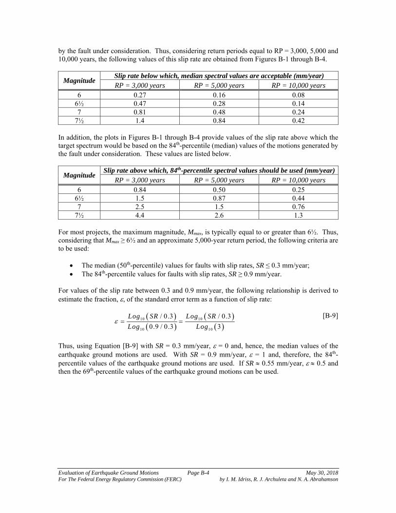
Evaluation of Earthquake Ground Motions Page B-4 May 30, 2018 For The Federal Energy Regulatory Commission (FERC) by I. M. Idriss, R. J. Archuleta and N. A. Abrahamson
by the fault under consideration. Thus, considering return periods equal to RP = 3,000, 5,000 and 10,000 years, the following values of this slip rate are obtained from Figures B-1 through B-4.
Magnitude Slip rate below which, median spectral values are acceptable (mm/year) RP = 3,000 years RP = 5,000 years RP = 10,000 years
6 0.27 0.16 0.08 6½ 0.47 0.28 0.14 7 0.81 0.48 0.24
7½ 1.4 0.84 0.42 In addition, the plots in Figures B-1 through B-4 provide values of the slip rate above which the target spectrum would be based on the 84th-percentile (median) values of the motions generated by the fault under consideration. These values are listed below.
Magnitude Slip rate above which, 84th-percentile spectral values should be used (mm/year)
RP = 3,000 years RP = 5,000 years RP = 10,000 years 6 0.84 0.50 0.25
6½ 1.5 0.87 0.44 7 2.5 1.5 0.76
7½ 4.4 2.6 1.3 For most projects, the maximum magnitude, Mmax, is typically equal to or greater than 6½. Thus, considering that Mmax ≥ 6½ and an approximate 5,000-year return period, the following criteria are to be used:
The median (50th-percentile) values for faults with slip rates, SR ≤ 0.3 mm/year; The 84th-percentile values for faults with slip rates, SR ≥ 0.9 mm/year.
For values of the slip rate between 0.3 and 0.9 mm/year, the following relationship is derived to estimate the fraction, , of the standard error term as a function of slip rate:
10 10
10 10
/ 0.3 / 0.3
0.9 / 0.3 3
Log SR Log SR
Log Log
[B-9]
Thus, using Equation [B-9] with SR = 0.3 mm/year, = 0 and, hence, the median values of the earthquake ground motions are used. With SR = 0.9 mm/year, = 1 and, therefore, the 84th-percentile values of the earthquake ground motions are used. If SR 0.55 mm/year, 0.5 and then the 69th-percentile values of the earthquake ground motions can be used.

Evaluation of Earthquake Ground Motions Page B-5 May 30, 2018 For The Federal Energy Regulatory Commission (FERC) by I. M. Idriss, R. J. Archuleta and N. A. Abrahamson
Slip rate (mm/year)
0.2 0.3 0.4 0.5 0.6 0.7 0.8 0.9 20.1 1
Ave
rag
e re
turn
per
iod
(ye
ar)
0
5000
10000
15000
20000Earthquake magnitude, M = 6
Median percentile earthquake ground motions
84th percentile earthquake ground motions
69th percentile earthquake ground motions
Figure B-1 Variations of average return period with average slip rate considering a seismic source whose maximum magnitude is Mmax = 6
Slip rate (mm/year)
0.2 0.3 0.4 0.5 0.6 0.7 0.8 0.9 20.1 1
Ave
rag
e re
turn
pe
rio
d (
year
)
0
5000
10000
15000
20000Earthquake magnitude, M = 6.5
Median percentile earthquake ground motions
84th percentile earthquake ground motions
69th percentile earthquake ground motions
Figure B-2 Variations of average return period with average slip rate considering a seismic source whose maximum magnitude is Mmax = 6½

Evaluation of Earthquake Ground Motions Page B-6 May 30, 2018 For The Federal Energy Regulatory Commission (FERC) by I. M. Idriss, R. J. Archuleta and N. A. Abrahamson
Slip rate (mm/year)
0.2 0.3 0.4 0.5 0.6 0.7 0.8 0.9 20.1 1
Ave
rag
e re
turn
per
iod
(ye
ar)
0
5000
10000
15000
20000
Median percentile earthquake ground motions
84th percentile earthquake ground motions
69th percentile earthquake ground motions
Earthquake magnitude, M = 7
Figure B-3 Variations of average return period with average slip rate considering a seismic source whose maximum magnitude is Mmax = 7
Slip rate (mm/year)
0.2 0.3 0.4 0.5 0.6 0.7 0.8 0.9 20.1 1
Ave
rag
e re
turn
per
iod
(ye
ar)
0
5000
10000
15000
20000
Median percentile earthquake ground motions
84th percentile earthquake ground motions
69th percentile earthquake ground motions
Earthquake magnitude, M = 7.5
Figure B-4 Variations of average return period with average slip rate considering a seismic source whose maximum magnitude is Mmax = 7½

Evaluation of Earthquake Ground Motions Page C-1 May 30, 2018 For The Federal Energy Regulatory Commission (FERC) by I. M. Idriss, R. J. Archuleta and N. A. Abrahamson
APPENDIX C EXAMPLES – PROBABILISTIC SEISMIC HAZARD ANALYSIS
C.1 INTRODUCTION This appendix describes the types of results that should be obtained from a probabilistic seismic hazard analysis (PSHA) and in the development of time histories for possible dynamic analyses. The standard equations for conducting the PSHA and time history development are summarized in Section 4.2 of this report. The emphasis in this appendix is on the results of a PSHA and on the presentation of these results. The details for developing realistic scenario earthquake spectra are described in this Appendix since this has not been part of a standard PSHA practice until recently. The results of probabilistic seismic hazard analyses for two sites are presented in this Appendix. One site is located in a high activity region (San Francisco Bay Area) and the other site is located in a moderate activity region (Pacific Northwest). C.2 KEY COMPONENTS NEEDED FOR A PSHA The key components needed for a PSHA are: source characterization; maximum magnitude; GMMs (attenuation relationships); hazard results; and de-aggregation. Each of these components is described in more detail below. C.2.1 Source Characterization The source characterization should include a description of the key sources and a map of faults and source zones. It should also incorporate the historical seismicity. A table should be provided to provide the fault and source zone parameters used in the PSHA, including alternatives models and parameter values with their associated weights. C.2.2 Maximum Magnitude Inconsistent use of terminology is a cause of confusion in many PSHA reports. In listing the fault and source zone parameters, the term "maximum magnitude" is often used for both the true maximum magnitude and for the mean magnitude from full rupture of a fault. For source zones, the maximum magnitude is the largest magnitude that can occur in the source zone. If an exponential distribution is used for the magnitudes (e.g. Gutenberg-Richter model), then the maximum magnitude is the magnitude at which the exponential distribution is truncated. For faults, the dimension of the fault (length or area) is typically used to estimate the mean magnitude for full rupture of the fault. This mean magnitude is better described as the "mean characteristic magnitude" and not as the maximum magnitude because the PSHA will typically consider a range of values about this mean magnitude to account for the variability of the magnitude for a given rupture dimension. For example, the widely used Youngs and Coppersmith (1985) model for the magnitude distribution has the characteristic part of the model centered on the mean characteristic magnitude and the maximum magnitude is 0.25 units larger. C.2.3 Ground Motion Models In most cases, the earthquake ground motions models are selected from existing models for the appropriate tectonic regime (shallow crustal earthquakes in active tectonic regions, shallow crustal earthquakes in stable continental regions, or subduction zone earthquakes). Alternative models that

Evaluation of Earthquake Ground Motions Page C-2 May 30, 2018 For The Federal Energy Regulatory Commission (FERC) by I. M. Idriss, R. J. Archuleta and N. A. Abrahamson
are considered applicable should be used to capture the epistemic uncertainty in the ground motion models. The PSHA report needs to describe the weights used for each model. In some cases, new ground motion models are derived for a specific project using either empirical data or numerical simulations (see Appendix E for more details regarding numerical procedures). If new project-specific ground motion model is derived, a full description of the development and justification of the new model should be included. C.2.4 Hazard Results The basic result of a PSHA is the hazard curve, which shows the probability of exceeding a ground motion parameter (PGA, spectral acceleration at a specified period … etc.) for a range of ground motion values. As a minimum, the hazard should be shown for a least two spectral periods: one short period, such as PGA, and one long period, such as T = 1 or 2 sec. The selection of the spectral periods should consider the period of interest for the project. Either the best estimate (median or 50-percentile) or the mean hazard curves should be plotted to show the hazard curve from each source and the total hazard curve to provide insight into which sources are most important. The median or mean hazard curves should also be shown in terms of the total hazard using each ground motion model (GMM) separately to show the impact of the different ground motion models. Finally, the fractiles of the hazard should be plotted to show the range of hazard that arises due to the uncertainty in the characterization of the sources and ground motion. C.2.5 De-aggregation The hazard curve gives the combined effect of all magnitudes and distances on the probability of exceeding a given ground motion level. Since all of the sources, magnitudes, and distances are mixed together, it is difficult to get an intuitive understanding of what is controlling the hazard from the hazard curve alone. To provide insight into what events are the most important for the hazard at a given ground motion level, the hazard curve is broken down into its contributions from different earthquake scenarios. This process is called de-aggregation. In a hazard calculation, there is a large number of scenarios considered (e.g. thousands or millions of scenarios). To reduce this large number of scenarios to a manageable number, similar scenarios are grouped together. A key issue is what constitutes "similar" scenarios. Typically, little thought has been given to the grouping of the scenarios. Most hazard studies use equal spacing in magnitude space and distance space. This may not be appropriate for a specific project. The selection of the grouping of scenarios should be defined by the engineers conducting the analysis for the project. In a de-aggregation, the fractional contribution of different scenario groups to the total hazard is computed. The most common form of de-aggregation is a two-dimensional de-aggregation in magnitude and distance bins. The dominant scenario can be characterized by an average of the de-aggregation. Two types of averages are considered: the mean and the mode. The mean magnitude and mean distance are the weighted averages with the weights given by the de-aggregation (i.e., contribution of the magnitude bin and contribution of the distance bin, respectively). The mean has advantages in that it is defined unambiguously and is simple to compute. The disadvantage is that it may give a value that does not correspond to a realistic scenario.
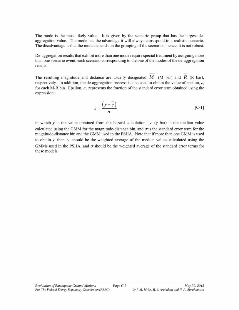
Evaluation of Earthquake Ground Motions Page C-3 May 30, 2018 For The Federal Energy Regulatory Commission (FERC) by I. M. Idriss, R. J. Archuleta and N. A. Abrahamson
The mode is the most likely value. It is given by the scenario group that has the largest de-aggregation value. The mode has the advantage it will always correspond to a realistic scenario. The disadvantage is that the mode depends on the grouping of the scenarios; hence, it is not robust. De-aggregation results that exhibit more than one mode require special treatment by assigning more than one scenario event, each scenario corresponding to the one of the modes of the de-aggregation results.
The resulting magnitude and distance are usually designated M (M bar) and R (R bar), respectively. In addition, the de-aggregation process is also used to obtain the value of epsilon, , for each M-R bin. Epsilon, , represents the fraction of the standard error term obtained using the expression:
y y
[C-1]
in which y is the value obtained from the hazard calculation, y (y bar) is the median value
calculated using the GMM for the magnitude-distance bin, and is the standard error term for the magnitude-distance bin and the GMM used in the PSHA. Note that if more than one GMM is used to obtain y, then y should be the weighted average of the median values calculated using the
GMMs used in the PSHA, and should be the weighted average of the standard error terms for these models.

Evaluation of Earthquake Ground Motions Page C-4 May 30, 2018 For The Federal Energy Regulatory Commission (FERC) by I. M. Idriss, R. J. Archuleta and N. A. Abrahamson
C.3 UNIFORM HAZARD SPECTRA A common method for developing design spectra based on the probabilistic approach is the use of uniform hazard spectra. A uniform hazard spectrum (UHS) is developed by first computing the hazard at a suite of spectral periods using response spectral attenuation relations. That is, the hazard is computed independently for each spectral period. For a selected return period (see Section 4.2 for definition of return period), the spectral ordinate for each spectral period is selected from the hazard curves. These spectral ordinates are then plotted as a function of period to form the uniform hazard spectrum (UHS). The term "uniform hazard spectrum" is used because there is an equal probability of exceeding the spectral value at any period. Since the hazard is computed independently for each spectral period, a uniform hazard spectrum does not represent the spectrum of any single event. It is common to find that the short period (T < 0.2 sec) ground motions are controlled by nearby moderate magnitude earthquakes, whereas, the long period (T > 1 sec) ground motions are more likely controlled by distant large magnitude earthquakes. The "mixing" of earthquakes in the UHS is often cited as a disadvantage of PSHA. There is nothing in the PSHA methodology that requires using a UHS. Instead, a suite of realistic scenario earthquake spectra can be developed as described in Section C.4. The reason for using a UHS rather than using multiple spectra for the individual scenarios has been to reduce the number of analyses required. A deterministic analysis has the same issue. If one deterministic scenario leads to the largest spectral values for long spectral periods and a different deterministic scenario leads to the largest spectral values for short spectral periods, a single design spectrum that envelopes the two deterministic spectra could be developed but should be discouraged. If such an envelope is used, then the deterministic design spectrum also does not represent a single earthquake. In the latter case, it is best to utilize each deterministic spectrum separately in the design/evaluation of the project. The choice of using a UHS rather than multiple spectra for the different scenarios is the decision of the engineering analyst, not the hazard analyst. The engineering analyst should determine if it is worth the additional analysis costs to avoid exciting a broad period range in a single evaluation. The hazard report should include the UHS as well as the scenario spectra described in the next section. C.4 SPECTRA FOR SCENARIO EARTHQUAKES In addition to the UHS, realistic spectra for scenario earthquakes should be developed. Two different procedures for developing scenario earthquake spectra are described below. Both methods start with the identification of the controlling earthquake scenarios (magnitude, distance) from the de-aggregation plots. As noted above, the controlling earthquakes will change as a function of the spectral period and the hazard level (i.e., annual probability of exceedance or average return period).

Evaluation of Earthquake Ground Motions Page C-5 May 30, 2018 For The Federal Energy Regulatory Commission (FERC) by I. M. Idriss, R. J. Archuleta and N. A. Abrahamson
Median Spectral Shape The most common procedure used for developing scenario earthquake spectra given the results of a PSHA is to use the median spectral shape (Sa/PGA) for the earthquake scenario from the de-aggregation and then scale the median spectral shape so that it matches the UHS at the specified return period and spectral period. This process is repeated for a suite of spectral periods (e.g. T = 0.2 sec, T = 1 sec, T = 2.0 sec). The envelope of the resulting scenario spectra becomes equal to the UHS if a full range of spectral periods of the scenarios is included. This avoids the problem of mixing different earthquake scenarios that control the short and long period ranges of the UHS. A short-coming of the median spectral shape method is that it assumes that the variability of the ground motion is fully correlated over all spectral periods. For example, if the UHS at a specified spectral period and return period corresponds to the median plus 1 sigma ground motion for the scenario (i.e., =1), then by scaling the median spectral shape, the "median plus one sigma" spectral value is being used at each period. Spectra from real earthquakes will have peaks and troughs; therefore, it would not be expected that the spectrum will be at the "median plus one sigma" level at all periods. This short-coming is addressed in the second method. Expected Spectral Shape In this method, the expected spectral shape for the scenario earthquake is computed. This expected spectral shape depends not only on the scenario earthquake, but also on the epsilon value required to scale the scenario spectrum to the UHS. Again, consider a case in which the UHS is one standard deviation above the median spectral acceleration from the scenario earthquake for a period of 2 sec. At other spectral periods, the chance that the ground motion will also be at the 1 sigma level decreases as the spectral period moves farther from 2 sec. The correlation of the variability of the spectral values at different periods is needed to compute the expected spectral shape. Note that this refers to the correlation of the variability of the spectral values and not the correlation of the median values. In the past, this correlation has not been commonly included as part of the ground motion model, but the correlation tends to be only weakly dependent on the data set. That is, special studies that have developed this correlation can be applied to a range of ground motion models. The equations for obtaining the correlation are given below. The number of standard deviations,
,U o RPT T , needed to scale the median scenario spectral value to the UHS at a spectral period,
oT , and for a return period, RPT , is calculated using the following expression:
^
, , ,,
,
ao RP o
U o RPo
Ln UHS T T Ln S M R TT T
T M
[C-2]
In which ^
, ,a oS M R T and ,oT M are the median and standard deviation of the ground
motion for the scenario earthquake from the earthquake ground motions models (attenuation
relations). Note that ,o RPUHS T T is the same as y and ^
, ,a oS M R T is the same as y in
equation C-1.
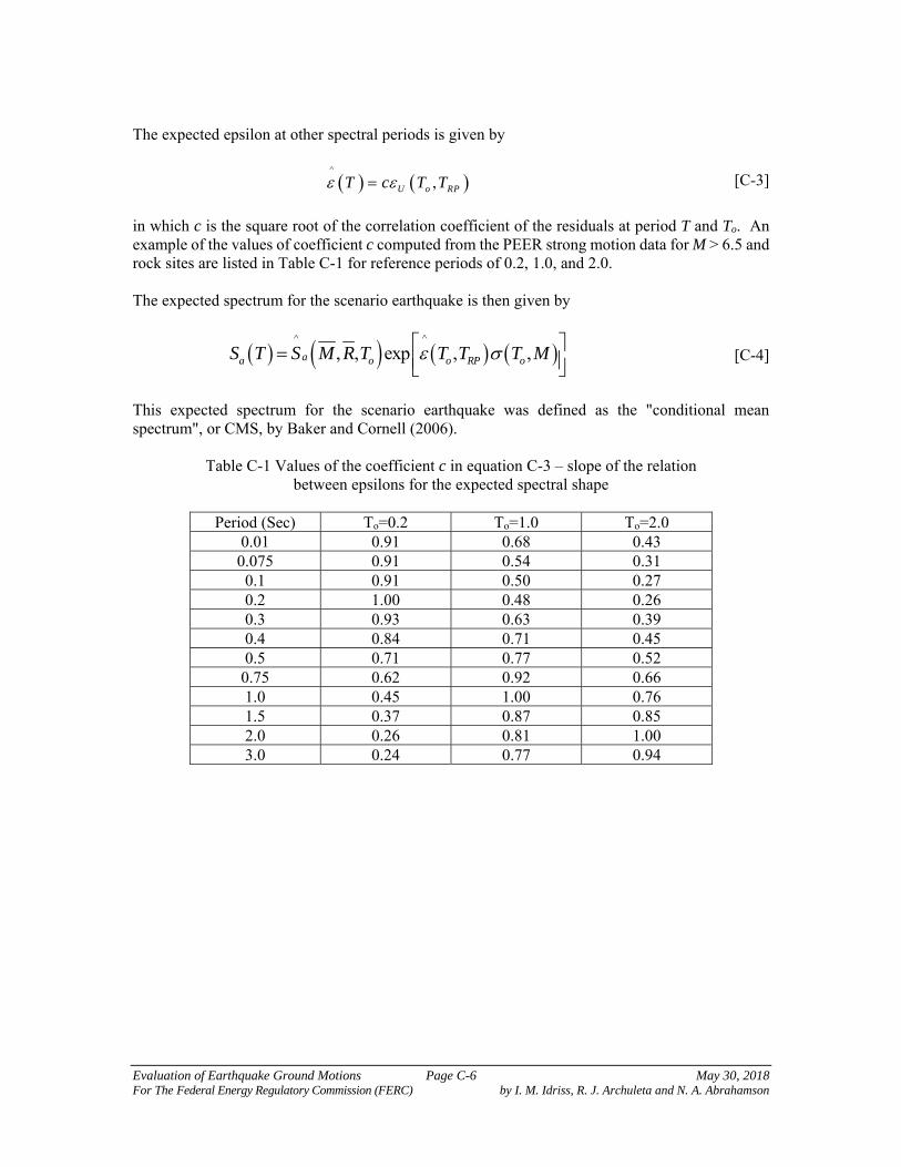
Evaluation of Earthquake Ground Motions Page C-6 May 30, 2018 For The Federal Energy Regulatory Commission (FERC) by I. M. Idriss, R. J. Archuleta and N. A. Abrahamson
The expected epsilon at other spectral periods is given by
^
,U o RPT c T T [C-3]
in which c is the square root of the correlation coefficient of the residuals at period T and To. An example of the values of coefficient c computed from the PEER strong motion data for M > 6.5 and rock sites are listed in Table C-1 for reference periods of 0.2, 1.0, and 2.0. The expected spectrum for the scenario earthquake is then given by
^ ^
, , exp , ,aa o o RP oS T S M R T T T T M [C-4]
This expected spectrum for the scenario earthquake was defined as the "conditional mean spectrum", or CMS, by Baker and Cornell (2006).
Table C-1 Values of the coefficient c in equation C-3 – slope of the relation between epsilons for the expected spectral shape
Period (Sec) To=0.2 To=1.0 To=2.0
0.01 0.91 0.68 0.43 0.075 0.91 0.54 0.31 0.1 0.91 0.50 0.27 0.2 1.00 0.48 0.26 0.3 0.93 0.63 0.39 0.4 0.84 0.71 0.45 0.5 0.71 0.77 0.52
0.75 0.62 0.92 0.66 1.0 0.45 1.00 0.76 1.5 0.37 0.87 0.85 2.0 0.26 0.81 1.00 3.0 0.24 0.77 0.94

Evaluation of Earthquake Ground Motions Page C-7 May 30, 2018 For The Federal Energy Regulatory Commission (FERC) by I. M. Idriss, R. J. Archuleta and N. A. Abrahamson
C.5 TIME HISTORIES Time histories are developed using the spectral matching approach for the Pacific Northwest example and using the scaling approach for the northern California example. The basis for selecting the reference time histories (sometimes designated "seed" time histories) should be described. One draw-back of using the expected scenario spectra is that additional time histories will be required. If the project will be using the average response of 7 time histories, then 7 time histories are needed for each scenario spectrum. The average response is computed for each scenario and then the larger response from the two scenario is used. If the scaling procedure is used, then the time history report should list the scale factors and include the following plots:
Acceleration, velocity, and displacement seismograms for the scaled time histories. Fourier amplitude spectra for the scaled time histories. Comparison of the spectra of the scaled time histories with the design spectrum.
If the spectral matching procedure is used, then there are additional plots that are needed to check that the modified time history is still appropriate (e.g. check that the spectral matching has not lead to an unrealistic ground motion). The acceleration, velocity, and displacement seismograms of the modified ground motion should have the same gross non-stationary characteristics as the reference motion. For spectral matching, the time history report should include the following plots:
Acceleration, velocity, and displacement seismograms for the reference and modified time histories.
Fourier amplitude spectra for the reference and modified time histories. Comparison of Husid plots (normalized arias intensity) for the reference and modified time
histories. Comparison of the spectra of the reference and modified time histories with the scenario
earthquake spectrum. C.6 EXAMPLES OF PROBABILISTIC SEISMIC HAZARD ANALYSIS C.6.1 San Francisco Bay Area The first example is for a site located in the East Bay in Northern California, which is in a high seismic region. The return period of 2,000 years is used only for illustration purposes and does not imply that it is an accepted return period for dams. Source Characterization For this example, a simplified source characterization is used. Three fault sources are considered: (i) the San Andreas; (ii) the Hayward/Rodgers Creek; and (iii) the Calaveras faults. The location of the site with respect to these faults is shown in Figure C-1. The parameters used for the sources are given in Table C-2. These parameters are based on the USGS WG03 model. The objective of these examples is on the presentation of the hazard results, so a detailed description of the source models is not included here. In a complete hazard study, such detailed source descriptions should be included.

Evaluation of Earthquake Ground Motions Page C-8 May 30, 2018 For The Federal Energy Regulatory Commission (FERC) by I. M. Idriss, R. J. Archuleta and N. A. Abrahamson
Ground Motion Models For the crustal sources, the five NGA models recently developed as part of the PEER/Lifelines program are used. These are the earlier 2008 ground motion models by Abrahamson and Silva, Boore and Atkinson, Campbell and Bozorgnia, Chiou and Youngs, and Idriss. For the Idriss model, the rock site class is used. For the other four models, a VS30 = 600 m/s is used. These five models are given equal weight.
Table C-2 Source parameters for faults considered for the San Francisco Example
Fault System Rupture Mean
Characteristic Magnitude (weight)
Recurrence Interval (year)
of Characteristic Earthquake (weight)
Style-of-Faulting
San Andreas SAS 7.03 (0.8) 6.84 (0.1) 7.22 (0.1)
1,140(0.8) 260 (0.1)
100,000 (0.1) Strike-Slip
San Andreas SAP 7.15 (0.8) 6.95 (0.1) 7.32 (0.1)
670 (0.8) 160 (0.1)
100,000 (0.1) Strike-Slip
San Andreas SAN 7.45 (0.8) 7.28 (0.1) 7.61 (0.1)
3,320 (0.8) 800(0.1)
100,000 (0.1) Strike-slip
San Andreas SAO 7.29 (0.8) 7.12 (0.1) 7.44 (0.1)
3320 (0.8) 680 (0.1)
100,000 (0.1) Strike-slip
San Andreas SAS + SAP 7.42 (0.8) 7.26 (0.1) 7.56 (0.1)
840 (0.8) 30,000 (0.1)
280 (0.1) Strike-slip
San Andreas SAN + SAO 7.70 (0.8) 7.53 (0.1) 7.86 (0.1)
870 (0.8) 30,000 (0.1)
270 (0.1) Strike-slip
San Andreas SAS + SAP +
SAN
7.76 (0.8) 7.59 (0.1) 7.92 (0.1)
30,000 (0.8) 10,000 (0.1)
100,000 (0.1) Strike-slip
San Andreas SAP + SAN +
SAO
7.83 (0.8) 7.65 (0.1) 8.01 (0.1)
15,000 (0.8) 2700 (0.1)
100,000 (0.1) Strike-slip
San Andreas SAS + SAP + SAN + SAO
7.90 (0.8) 7.72 (0.1) 8.10 (0.1)
620 (0.8) 10,000 (0.1)
200 (0.1) Strike-slip
San Andreas Floating 6.9 (0.1) 410 (0.8)
7,500 (0.1) 100 (0.1)
Strike-slip
Hayward/RC HS 6.67 (0.8) 6.36 (0.1) 6.93 (0.1)
250 (0.8) 1350 (0.1)
80 (0.1) Strike-slip
HN 6.49 (0.8) 6.18 (0.1) 6.78 (0.1)
230 (0.8) 1290 (0.1)
70 (0.1) Strike-slip

Evaluation of Earthquake Ground Motions Page C-9 May 30, 2018 For The Federal Energy Regulatory Commission (FERC) by I. M. Idriss, R. J. Archuleta and N. A. Abrahamson
HS + HN 6.91 (0.8) 6.68 (0.1) 7.12 (0.1)
340 (0.8) 1560 (0.1) 110 (0.1)
Strike-slip
RC 6.98 (0.8) 6.81 (0.1) 7.14 (0.1)
180 (0.8) 720 (0.1) 56 (0.1)
Strike-slip
HN + RC 7.11 (0.8) 6.94 (0.1) 7.28 (0.1)
1650 (0.8) 440 (0.1)
100,000 (0.1) Strike-slip
HN + RS + RC 7.26 (0.8) 7.09 (0.1) 7.42 (0.1)
3,000(0.8) 30,000 (0.1)
900 (0.1) Strike-slip
Floating 6.90 (1.0)
4270 (0.8) 10,000 (0.1) 1860 (0.1)
Strike-slip
Calaveras CS 5.79 (0.8) 5.0 (0.1)
6.14 (0.1)
125 (0.8) 40 (0.1)
100,000 (0.1) Strike-slip
CC 6.23 (0.8) 5.75 (0.1) 6.68 (0.1)
200 (0.8) 750 (0.1) 85 (0.1)
Strike-slip
CS + CC 6.36 (0.8) 5.87 (0.1) 6.75 (0.1)
590 (0.8) 130 (0.1)
100,000 (0.1) Strike-slip
CN 6.78 (0.8) 6.58 (0.1) 6.97 (0.1)
230 (0.8) 990 (0.1) 70 (0.1)
Strike-slip
CC + CN 6.90 (0.8) 6.68 (0.1) 7.11 (0.1)
10,000 (0.8) 820 (0.1)
100,000 (0.1) Strike-slip
CS + CC + CN 6.93 (0.8) 6.72 (0.1) 7.14 (0.1)
1490 (0.8) 370 (0.1)
100,000 (0.1) Strike-slip
Floating 6.20 (1.0)
390 (0.8) 1750 (0.1) 140 (0.1)
Strike-slip
CS + CC floating
6.2 (1.0) 100 (0.8) 570 (0.1) 40 (0.1)
Strike-slip
Note to the reader: The examples included in this Appendix were completed in 2007, about a year before the NGA relationships were published in Spectra in February 2008. The models used for these examples were slightly modified before final publication in Spectra. Thus, the actual results of the PSHA would be somewhat different from those presented in this Appendix. However, the conclusions and the value of the example are not diminished. The examples are provided in this appendix as illustration of the methodology, and hence there is no need to update the results using the most current relationships. For real applications, the most current relationships need to be used following the guidance summarized in Appendix D.

Evaluation of Earthquake Ground Motions Page C-10 May 30, 2018 For The Federal Energy Regulatory Commission (FERC) by I. M. Idriss, R. J. Archuleta and N. A. Abrahamson
Hazard Results The basic hazard results are shown in Figures C-2a and C-2b for PGA and T=1 sec, respectively. These figures also show how each source contributes to the hazard. Since the site is located close to a high activity fault, the hazard is dominated by the nearby Hayward fault at both short and long spectral periods. The sensitivity of the hazard to the attenuation relations is shown in Figure C-3a and C-3b for PGA and T = 1 sec, respectively. As the return period increases (lower annual probability), the difference due to the attenuation relation increases. This is due to the different values of the standard deviations. The epistemic uncertainty in the hazard is shown in Figures C-4a and C-4b for PGA and T = 1 sec, respectively. The UHS for return periods of 500, 1000, 2000, and 5000 years is shown in Figure C-5. This figure also compares the Hayward MCE (M = 7.25, R=3.5 km) ground motions (median and 84th percentile) as used in deterministic analyses. At short spectral periods, the 84th percentile ground motion is close to the UHS at return period of about 700 years. This increases to a return period of 2000 years at long spectral periods. The de-aggregation for a return period of 2000 years is shown in Figures C-6a and C-6b for PGA and T = 1 sec, respectively. Figure C-6a shows that for PGA, the mode of the de-aggregation is M = 6.5-7.0 at a distance of 0-5 km. Figure C-6b shows that for T=1 sec, the mode of the de-aggregation is still M = 6.5-7.0 at a distance of 0-5 km, but the contribution of larger magnitudes (M = 7.0-7.5) has increased. If the bin size were changed, the model may move to M = 7. This shows how simply using the mode can miss some changes in the controlling source. In addition to the mode, the de-aggregation can be characterized by the mean magnitude, distance, and epsilon. These mean values are shown in Figure C-7 as a function of return period for PGA and T = 1 sec. With this type of plot, the differences in the magnitude for PGA and T = 2 sec is apparent. As is typical for sites close to active faults, the mean magnitude is not very sensitive to the return period. At short spectral periods, the mean distance decreases quickly to the closest distance (3.5 km in this case). The main increase in the ground motion at long return periods is due to the increase in epsilon shown in the lower frame. Expected Spectra for Scenario Earthquakes From the de-aggregation, the following scenario earthquakes were selected: Source M Distance (km) To (sec) Hayward (SH) 6.75 4 km 0.2 Hayward (NS + SH) 7.0 5 km 1.0 The expected spectra, or conditional mean spectra (CMS), are developed for these events. First, the median and standard deviation for the two scenarios listed above are computed using the five NGA ground motion models. The average of the median and the standard deviation for the two scenario earthquakes are listed in Tables C-4a and C-4b. Next, the number of standard deviations needed to scale the median Sa to the UHS is determined. This value, U, is shown in Table C-3. The expected epsilon values at the other spectral periods are

Evaluation of Earthquake Ground Motions Page C-11 May 30, 2018 For The Federal Energy Regulatory Commission (FERC) by I. M. Idriss, R. J. Archuleta and N. A. Abrahamson
then computed (fifth column in Tables C-4a and C-4b) and the spectrum is then computed (sixth column in Tables C-4a, and C-4b). The expected spectra for the scenarios are compared to the UHS in Figure C-8. This figure shows that even if there is a single controlling source, the expected spectrum will still fall below the UHS at periods away from the reference period. This shows that it is not just the enveloping of earthquakes from different sources in the UHS, but also the enveloping of the variability at different spectral periods. A suite of these expected spectra will be enveloped by the UHS. The expected spectra are realistic ground motions for a future earthquake. To limit the number of scenarios considered, these expected spectra can be broadened so that they cover the UHS with a small number of scenarios. As an example, the two expected scenarios are broadened into two design spectra in Figure C-9. The engineer conducting the analysis of the structure needs to determine to what degree it is worth broadening the expected spectra to reduce the number of scenarios considered.
Table C-3 Computation of the epsilon needed to match the UHS
Period (sec)
UHS 2000 Years
(g) Median Sa(g) U
0.2 2.56 0.904 0.619 1.68 1.0 0.97 0.313 0.660 1.72

Evaluation of Earthquake Ground Motions Page C-12 May 30, 2018 For The Federal Energy Regulatory Commission (FERC) by I. M. Idriss, R. J. Archuleta and N. A. Abrahamson
Table C-4a. Development for the expected spectrum for T=0.2 sec and a return period of 2000 years.
Period (Sec) c
(To=0.2) Median Sa(g) ̂
Expected Spectrum
(g) 0.00 0.91 0.388 0.560 1.530 0.913 0.075 0.91 0.608 0.625 1.530 1.584 0.10 0.91 0.736 0.633 1.530 1.938 0.20 1.00 0.904 0.619 1.682 2.560 0.30 0.93 0.820 0.630 1.564 2.196 0.40 0.84 0.693 0.635 1.413 1.699 0.50 0.71 0.603 0.640 1.194 1.294 0.75 0.62 0.412 0.650 1.043 0.811 1.00 0.45 0.313 0.662 0.757 0.516 1.50 0.37 0.206 0.675 0.622 0.314 2.00 0.26 0.140 0.693 0.437 0.190 3.00 0.24 0.083 0.697 0.404 0.110
Table C-4b. Development for the expected spectrum for T=1.0 sec and a return period of 2000 years.
Period (Sec) c
(To=1.0) Median Sa(g) ̂
Expected Spectrum
(g) 0.00 0.68 0.374 0.554 1.167 0.745 0.075 0.54 0.587 0.620 0.927 1.086 0.10 0.5 0.703 0.626 0.858 1.267 0.20 0.48 0.876 0.613 0.824 1.505 0.30 0.63 0.801 0.625 1.081 1.620 0.40 0.71 0.677 0.630 1.218 1.502 0.50 0.77 0.600 0.636 1.321 1.404 0.75 0.92 0.410 0.650 1.579 1.149 1.00 1.00 0.322 0.660 1.716 0.974 1.50 0.87 0.213 0.675 1.493 0.565 2.00 0.81 0.150 0.691 1.390 0.368 3.00 0.77 0.090 0.696 1.321 0.208

Evaluation of Earthquake Ground Motions Page C-13 May 30, 2018 For The Federal Energy Regulatory Commission (FERC) by I. M. Idriss, R. J. Archuleta and N. A. Abrahamson
Figure C-1. Faults and sources considered in the example.

Evaluation of Earthquake Ground Motions Page C-14 May 30, 2018 For The Federal Energy Regulatory Commission (FERC) by I. M. Idriss, R. J. Archuleta and N. A. Abrahamson
Figure C-2a. Contribution to the PGA hazard by source.
Figure C-2b. Contribution to the T=1 sec hazard by source
0.0001
0.001
0.01
0.1
0 0.2 0.4 0.6 0.8 1 1.2 1.4
Ann
ual P
roba
bilit
y of
Bei
ng E
xcee
ded
PGA (g)
San Andreas
Hayward
Calaveras
Other faults
Total
0.0001
0.001
0.01
0.1
0 0.2 0.4 0.6 0.8 1 1.2 1.4
Ann
ual P
roba
bilit
y of
Bei
ng E
xcee
ded
Sa (g)
SanAndreas
Hayward
Calaveras
Other faults
Total

Evaluation of Earthquake Ground Motions Page C-15 May 30, 2018 For The Federal Energy Regulatory Commission (FERC) by I. M. Idriss, R. J. Archuleta and N. A. Abrahamson
Figure C-3a. Sensitivity of PGA hazard to attenuation relation.
Figure C-3b. Sensitivity of T=1 sec hazard to attenuation relation.
0.0001
0.001
0.01
0.1
0 0.5 1 1.5
Ann
ual P
roba
bilit
y of
Bei
ng E
xcee
ded
Peak Acceleration (g)
Abrahamson & Silva
Chiou & Youngs
Boore & Atkinson
Campbell & Bozorgnia
Idriss
0.0001
0.001
0.01
0.1
0 0.5 1 1.5
Ann
ual P
roba
bilit
y of
Bei
ng E
xcee
ded
Spectral Acceleration (g)
Abrahamson & Silva
Chiou & Youngs
Boore & Atkinson
Campbell & Bozorgnia
Idriss

Evaluation of Earthquake Ground Motions Page C-16 May 30, 2018 For The Federal Energy Regulatory Commission (FERC) by I. M. Idriss, R. J. Archuleta and N. A. Abrahamson
Figure C-4a. Uncertainty fractiles of the PGA hazard
Figure C-4b. Uncertainty fractiles of the T=1 sec hazard
0.0001
0.001
0.01
0.1
0 0.2 0.4 0.6 0.8 1 1.2 1.4 1.6 1.8 2
Pro
babi
lity
of B
eing
Exc
eede
d
Peak Acceleration (g)
5th
15th
50th
85th
95th
Mean
0.0001
0.001
0.01
0.1
0 0.2 0.4 0.6 0.8 1 1.2 1.4 1.6 1.8 2
Pro
babi
lity
of B
eing
Exc
eede
d
Spectral Acceleration (g)
5th
15th
50th
85th
95th
Mean

Evaluation of Earthquake Ground Motions Page C-17 May 30, 2018 For The Federal Energy Regulatory Commission (FERC) by I. M. Idriss, R. J. Archuleta and N. A. Abrahamson
Figure C-5. UHS and deterministic (MCE) spectra for the Hayward/Rodgers Creek source.
0
0.5
1
1.5
2
2.5
3
3.5
0.01 0.1 1 10
Spe
ctra
l Acc
eler
atio
n (g
)
Period (sec)
500 Yr
1000 Yr
2000 Yr
5000 Yr
Hayward Median (M7.25)
Hayward 84th (M7.25)
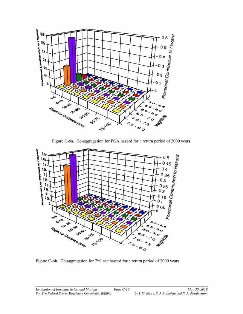
Evaluation of Earthquake Ground Motions Page C-18 May 30, 2018 For The Federal Energy Regulatory Commission (FERC) by I. M. Idriss, R. J. Archuleta and N. A. Abrahamson
Figure C-6a. De-aggregation for PGA hazard for a return period of 2000 years.
Figure C-6b. De-aggregation for T=1 sec hazard for a return period of 2000 years.
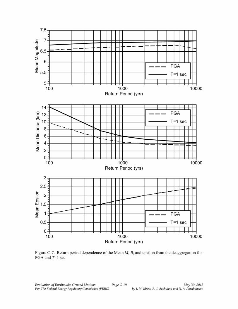
Evaluation of Earthquake Ground Motions Page C-19 May 30, 2018 For The Federal Energy Regulatory Commission (FERC) by I. M. Idriss, R. J. Archuleta and N. A. Abrahamson
Figure C-7. Return period dependence of the Mean M, R, and epsilon from the deaggregation for PGA and T=1 sec
5
5.5
6
6.5
7
7.5
100 1000 10000
Me
an
Ma
gn
itud
e
Return Period (yrs)
PGA
T=1 sec
0
2
4
6
8
10
12
14
100 1000 10000
Mea
n D
ista
nce
(km
)
Return Period (yrs)
PGA
T=1 sec
0
0.5
1
1.5
2
2.5
3
100 1000 10000
Me
an
Ep
silo
n
Return Period (yrs)
PGA
T=1 sec

Evaluation of Earthquake Ground Motions Page C-20 May 30, 2018 For The Federal Energy Regulatory Commission (FERC) by I. M. Idriss, R. J. Archuleta and N. A. Abrahamson
Figure C-8. Expected spectra for scenario earthquakes for the UHS at T=0.2 and T=1.0 sec.
0
0.5
1
1.5
2
2.5
3
0.01 0.1 1 10
Spe
ctra
l Acc
eler
atio
n (g
)
Period (sec)
2000 Yr UHS
Hayward (6.75)
Hayward (7.0)

Evaluation of Earthquake Ground Motions Page C-21 May 30, 2018 For The Federal Energy Regulatory Commission (FERC) by I. M. Idriss, R. J. Archuleta and N. A. Abrahamson
Figure C-9. Example of broadening the expected spectra for scenario earthquakes into a small set of design spectra.
0
0.5
1
1.5
2
2.5
3
0.01 0.1 1 10
2000 Yr UHS
Hayward (6.75)
Hayward (7.0)
Design Scenario 1
Design Scenario 2

Evaluation of Earthquake Ground Motions Page C-22 May 30, 2018 For The Federal Energy Regulatory Commission (FERC) by I. M. Idriss, R. J. Archuleta and N. A. Abrahamson
C.6.2 Pacific Northwest A site located in northwestern Washington is used as the second example. Again, a return period of 2000 years is used. As in the first example, the return period of 2,000 years is used only for illustration purposes and does not imply that it is an accepted return period for dams. Source Characterization For this example, a simplified source characterization is used. Five sources are considered: (i) the Cascadia interface; (ii) the Juan de Fuca intra-slab; (iii) the Seattle fault; (iv) the Hood Canal fault; and (v) a background zone. The location of the site with respect to the faults and source zones is shown in Figure C-10. The parameters used for the sources are given in Tables C-5a and C-5b. These parameters are based on the source models used by Adams and Halchuk (2003), and the USGS as part of the national hazard maps. The objective of these examples is the presentation of the hazard results; thus, a detailed description of the source models is not included here. In a complete hazard study, such detailed source descriptions should be included. Ground Motion Models In the Pacific Northwest, both crustal and subduction earthquakes need to be considered. These two tectonic classes of earthquakes require separate ground motion models. For the crustal sources, the five NGA models used in Section C.6.1 were also used for this example. The five models are given equal weight. Note to the reader: see discussion at the end of Section C.6.1 regarding the NGA ground motion models. For the subduction earthquakes, two models are used: Youngs et al. (1997) and Atkinson and Boore (2003). For the Youngs et al. model, the rock relation is used. For the Atkinson and Boore model, NEHRP site class C is used. The two models are given equal weight. Note to the reader: These two ground motion attenuation relationships are no longer in use. As noted earlier in Section C.6.1, however, the examples are provided in this appendix as illustration of the methodology, and hence there is no need to update the results using the most current relationships. For applications, the most current relationships need to be used.
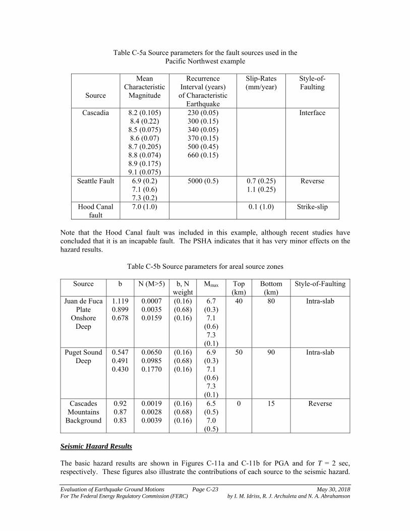
Evaluation of Earthquake Ground Motions Page C-23 May 30, 2018 For The Federal Energy Regulatory Commission (FERC) by I. M. Idriss, R. J. Archuleta and N. A. Abrahamson
Table C-5a Source parameters for the fault sources used in the Pacific Northwest example
Source
Mean Characteristic
Magnitude
Recurrence Interval (years)
of Characteristic Earthquake
Slip-Rates (mm/year)
Style-of-Faulting
Cascadia 8.2 (0.105) 8.4 (0.22)
8.5 (0.075) 8.6 (0.07)
8.7 (0.205) 8.8 (0.074) 8.9 (0.175) 9.1 (0.075)
230 (0.05) 300 (0.15) 340 (0.05) 370 (0.15) 500 (0.45) 660 (0.15)
Interface
Seattle Fault 6.9 (0.2) 7.1 (0.6) 7.3 (0.2)
5000 (0.5) 0.7 (0.25) 1.1 (0.25)
Reverse
Hood Canal fault
7.0 (1.0) 0.1 (1.0) Strike-slip
Note that the Hood Canal fault was included in this example, although recent studies have concluded that it is an incapable fault. The PSHA indicates that it has very minor effects on the hazard results.
Table C-5b Source parameters for areal source zones
Source b N (M>5) b, N weight
Mmax Top (km)
Bottom (km)
Style-of-Faulting
Juan de Fuca Plate
Onshore Deep
1.119 0.899 0.678
0.0007 0.0035 0.0159
(0.16) (0.68) (0.16)
6.7 (0.3) 7.1
(0.6) 7.3
(0.1)
40 80 Intra-slab
Puget Sound Deep
0.547 0.491 0.430
0.0650 0.0985 0.1770
(0.16) (0.68) (0.16)
6.9 (0.3) 7.1
(0.6) 7.3
(0.1)
50 90 Intra-slab
Cascades Mountains
Background
0.92 0.87 0.83
0.0019 0.0028 0.0039
(0.16) (0.68) (0.16)
6.5 (0.5) 7.0
(0.5)
0 15 Reverse
Seismic Hazard Results The basic hazard results are shown in Figures C-11a and C-11b for PGA and for T = 2 sec, respectively. These figures also illustrate the contributions of each source to the seismic hazard.
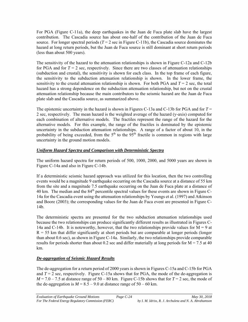
Evaluation of Earthquake Ground Motions Page C-24 May 30, 2018 For The Federal Energy Regulatory Commission (FERC) by I. M. Idriss, R. J. Archuleta and N. A. Abrahamson
For PGA (Figure C-11a), the deep earthquakes in the Juan de Fuca plate slab have the largest contribution. The Cascadia source has about one-half of the contribution of the Juan de Fuca source. For longer spectral periods (T = 2 sec in Figure C-11b), the Cascadia source dominates the hazard at long return periods, but the Juan de Fuca source is still dominant at short return periods (less than about 500 years). The sensitivity of the hazard to the attenuation relationships is shown in Figure C-12a and C-12b for PGA and for T = 2 sec, respectively. Since there are two classes of attenuation relationships (subduction and crustal), the sensitivity is shown for each class. In the top frame of each figure, the sensitivity to the subduction attenuation relationship is shown. In the lower frame, the sensitivity to the crustal attenuation relationship is shown. For both PGA and T = 2 sec, the total hazard has a strong dependence on the subduction attenuation relationship, but not on the crustal attenuation relationship because the main contributors to the seismic hazard are the Juan de Fuca plate slab and the Cascadia source, as summarized above. The epistemic uncertainty in the hazard is shown in Figures C-13a and C-13b for PGA and for T = 2 sec, respectively. The mean hazard is the weighted average of the hazard (y-axis) computed for each combination of alternative models. The fractiles represent the range of the hazard for the alternative models. For this example, the range of the fractiles is dominated by the epistemic uncertainty in the subduction attenuation relationships. A range of a factor of about 10, in the probability of being exceeded, from the 5th to the 95th fractile is common in regions with large uncertainty in the ground motion models. Uniform Hazard Spectra and Comparison with Deterministic Spectra The uniform hazard spectra for return periods of 500, 1000, 2000, and 5000 years are shown in Figure C-14a and also in Figure C-14b. If a deterministic seismic hazard approach was utilized for this location, then the two controlling events would be a magnitude 9 earthquake occurring on the Cascadia source at a distance of 55 km from the site and a magnitude 7.5 earthquake occurring on the Juan de Fuca plate at a distance of 40 km. The median and the 84th percentile spectral values for these events are shown in Figure C-14a for the Cascadia event using the attenuation relationships by Youngs et al. (1997) and Atkinson and Boore (2003); the corresponding values for the Juan de Fuca event are presented in Figure C-14b. The deterministic spectra are presented for the two subduction attenuation relationships used because the two relationships can produce significantly different results as illustrated in Figures C-14a and C-14b. It is noteworthy, however, that the two relationships provide values for M = 9 at R = 55 km that differ significantly at short periods but are comparable at longer periods (longer than about 0.6 sec), as shown in Figure C-14a. Similarly, the two relationships provide comparable results for periods shorter than about 0.2 sec and differ materially at long periods for M = 7.5 at 40 km. De-aggregation of Seismic Hazard Results The de-aggregation for a return period of 2000 years is shown in Figures C-15a and C-15b for PGA and T = 2 sec, respectively. Figure C-15a shows that for PGA, the mode of the de-aggregation is M = 7.0 – 7.5 at distance range of 50 – 80 km. Figure C-15b shows that for T = 2 sec, the mode of the de-aggregation is M = 8.5 – 9.0 at distance range of 50 – 60 km.

Evaluation of Earthquake Ground Motions Page C-25 May 30, 2018 For The Federal Energy Regulatory Commission (FERC) by I. M. Idriss, R. J. Archuleta and N. A. Abrahamson
In addition to the mode, the de-aggregation can be characterized by the mean magnitude, mean distance, and mean epsilon. These mean values are shown in Figure C-16 as a function of return period for PGA and for T = 2 sec. This figure shows that the mean magnitude for PGA increases slightly as the return period increases from 100 to 500 years, but for longer return periods, the mean magnitude does not increase. For return periods greater than 500 years, the mean distance continues to decrease slightly and the mean epsilon increases significantly. In contrast to the PGA, the mean magnitude for T = 2 sec continues to increase as the return period increases from 100 to 10,000 years. Expected Spectra for Scenario Earthquakes From the de-aggregation, the following scenario earthquakes were obtained: Source M Distance (km) To (sec) Juan de Fuca 7.3 50 km 0.2 Cascadia 8.8 55 km 2.0 The expected spectra are developed for these two events. First, the median and standard deviation for the two scenarios listed above are computed using the two subduction ground motion models. The average of the median and the standard deviation for the two scenario earthquakes are listed in Tables C-7a and C-7b. Next, the number of standard deviations needed to scale the median Sa to the UHS is determined. This value, U, is shown in Table C-6. The expected epsilon values at the other spectral periods are then computed (fifth column in Tables C-7a and C-7b) and the spectrum is then computed (sixth column in these tables). The expected spectra for the scenarios are compared to the UHS in Figure C-17. This figure shows that the expected spectrum falls below the UHS at periods away from the reference period. A suite of these expected spectra will be enveloped by the UHS. The expected spectra are realistic ground motions for a future earthquake. To limit the number of scenarios considered, these expected spectra will need to be broadened so that they cover the UHS with a small number of scenarios. As an example, the two expected scenarios are broadened into two design spectra in Figure C-18. The engineer conducting the analysis of the structure needs to determine to what extent it is worth broadening the expected spectra to reduce the number of scenarios considered.
Table C-6. Computation of the epsilon needed to match the UHS
Period (sec)
UHS 2000 Yr
(g) Median Sa(g) U
0.2 0.946 0.439 0.682 1.126 2.0 0.210 0.096 0.766 1.021

Evaluation of Earthquake Ground Motions Page C-26 May 30, 2018 For The Federal Energy Regulatory Commission (FERC) by I. M. Idriss, R. J. Archuleta and N. A. Abrahamson
Table C-7a. Development for the expected spectrum for T=0.2 sec and a return period of 2000 years
Period (Sec) c
(To=0.2) Median Sa(g) ̂
Expected Spectrum
(g) 0.00 0.91 0.192 0.625 1.024 0.364 0.075 0.91 0.269 0.648 1.024 0.522 0.10 0.91 0.314 0.671 1.024 0.624 0.20 1.00 0.439 0.682 1.126 0.947 0.30 0.93 0.419 0.691 1.047 0.864 0.40 0.84 0.400 0.694 0.946 0.771 0.50 0.71 0.389 0.706 0.799 0.683 0.75 0.62 0.286 0.720 0.698 0.472 1.00 0.45 0.218 0.751 0.507 0.319 1.50 0.37 0.147 0.770 0.417 0.202 2.00 0.26 0.107 0.801 0.293 0.135 3.00 0.24 0.050 0.874 0.270 0.063
Table C-7b. Development for the expected spectrum for T=2.0 sec and a return period of 2000 years
Period (Sec) c
(To=2.0) Median Sa(g) ̂
Expected Spectrum
(g) 0.00 0.43 0.144 0.590 0.439 0.186 0.075 0.31 0.211 0.611 0.317 0.256 0.10 0.27 0.237 0.636 0.276 0.282 0.20 0.26 0.320 0.647 0.266 0.380 0.30 0.39 0.321 0.650 0.399 0.416 0.40 0.45 0.361 0.659 0.460 0.488 0.50 0.52 0.346 0.676 0.531 0.495 0.75 0.66 0.248 0.696 0.674 0.396 1.00 0.76 0.188 0.716 0.777 0.327 1.50 0.85 0.130 0.742 0.869 0.248 2.00 1.00 0.096 0.766 1.022 0.211 3.00 0.94 0.037 0.839 0.961 0.082

Evaluation of Earthquake Ground Motions Page C-27 May 30, 2018 For The Federal Energy Regulatory Commission (FERC) by I. M. Idriss, R. J. Archuleta and N. A. Abrahamson
Figure C-10. Faults and sources considered in the example.

Evaluation of Earthquake Ground Motions Page C-28 May 30, 2018 For The Federal Energy Regulatory Commission (FERC) by I. M. Idriss, R. J. Archuleta and N. A. Abrahamson
Figure 11a. Contribution to the PGA hazard by source
Figure C-11b. Contribution to the T=2 sec hazard by source
0.0001
0.001
0.01
0.1
0 0.1 0.2 0.3 0.4 0.5 0.6 0.7
Ann
ual P
roba
bilit
y of
Bei
ng E
xcee
ded
Peak Acceleration (g)
Cascadia
Seattle Fault
Hood Canal fault
Juan de Fuca (Deep)
Background
Total
0.0001
0.001
0.01
0.1
0 0.05 0.1 0.15 0.2 0.25 0.3 0.35 0.4
Ann
ual P
roba
bilit
y of
Bei
ng E
xcee
ded
Spectral Acceleration (g)
Cascadia
Seattle Fault
Hood Canal fault
Juan de Fuca (Deep)
Background
Total

Evaluation of Earthquake Ground Motions Page C-29 May 30, 2018 For The Federal Energy Regulatory Commission (FERC) by I. M. Idriss, R. J. Archuleta and N. A. Abrahamson
Figure C-12a. Sensitivity of PGA hazard to attenuation relation. Top frame: subduction models. Bottom frame: crustal models
0.0001
0.001
0.01
0.1
0 0.1 0.2 0.3 0.4 0.5 0.6 0.7 0.8
Ann
ual P
roba
bilit
y of
Bei
ng E
xcee
ded
Peak Acceleration (g)
Youngs et al
Atkinson & Boore
0.0001
0.001
0.01
0.1
0 0.1 0.2 0.3 0.4 0.5 0.6 0.7 0.8
Ann
ual P
roba
bilit
y of
Bei
ng E
xcee
ded
Peak Acceleration (g)
Abrahamson & Silva
Chiou & Youngs
Boore & Atkinson
Campbell & Bozorgnia
Idriss
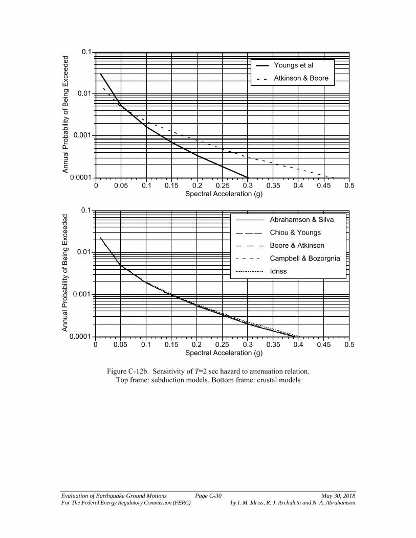
Evaluation of Earthquake Ground Motions Page C-30 May 30, 2018 For The Federal Energy Regulatory Commission (FERC) by I. M. Idriss, R. J. Archuleta and N. A. Abrahamson
Figure C-12b. Sensitivity of T=2 sec hazard to attenuation relation. Top frame: subduction models. Bottom frame: crustal models
0.0001
0.001
0.01
0.1
0 0.05 0.1 0.15 0.2 0.25 0.3 0.35 0.4 0.45 0.5
Ann
ual P
roba
bilit
y of
Bei
ng E
xcee
ded
Spectral Acceleration (g)
Youngs et al
Atkinson & Boore
0.0001
0.001
0.01
0.1
0 0.05 0.1 0.15 0.2 0.25 0.3 0.35 0.4 0.45 0.5
Ann
ual P
roba
bilit
y of
Bei
ng E
xcee
ded
Spectral Acceleration (g)
Abrahamson & Silva
Chiou & Youngs
Boore & Atkinson
Campbell & Bozorgnia
Idriss

Evaluation of Earthquake Ground Motions Page C-31 May 30, 2018 For The Federal Energy Regulatory Commission (FERC) by I. M. Idriss, R. J. Archuleta and N. A. Abrahamson
Figure 13a. Uncertainty fractiles of the PGA hazard
Figure C-13b. Uncertainty fractiles of the T=2 sec hazard
0.0001
0.001
0.01
0.1
0 0.1 0.2 0.3 0.4 0.5 0.6 0.7 0.8
Pro
babi
lity
of B
eing
Exc
eede
d
Peak Acceleration (g)
5th
15th
50th
85th
95th
Mean
0.0001
0.001
0.01
0.1
0 0.05 0.1 0.15 0.2 0.25 0.3 0.35 0.4 0.45 0.5
Pro
babi
lity
of B
eing
Exc
eede
d
Peak Acceleration (g)
5th
15th
50th
85th
95th
Mean

Evaluation of Earthquake Ground Motions Page C-32 May 30, 2018 For The Federal Energy Regulatory Commission (FERC) by I. M. Idriss, R. J. Archuleta and N. A. Abrahamson
Figure C-14a. UHS and deterministic (MCE) spectra for the M = 9 Cascadia source (R = 55 km).
0
0.5
1
1.5
0.01 0.1 1 10
Spe
ctra
l Acc
eler
atio
n (g
)
Period (sec)
500 Yr
1000 Yr
2000 Yr
5000 Yr
A&B Median (M9)
A&B 84th (M9)
Youngs et al median (M9)
Youngs et al 84th (M9)

Evaluation of Earthquake Ground Motions Page C-33 May 30, 2018 For The Federal Energy Regulatory Commission (FERC) by I. M. Idriss, R. J. Archuleta and N. A. Abrahamson
Figure C-14b. UHS and deterministic (MCE) spectra for the M = 7.6 Juan de Fuca source (R = 40 km)
0
0.5
1
1.5
0.01 0.1 1 10
Spe
ctra
l Acc
eler
atio
n (g
)
Period (sec)
500 Yr
1000 Yr
2000 Yr
5000 Yr
A&B Median (M7.5)
A&B 84th (M7.5)
Youngs et al Median, (M7.5)
Youngs et al 84th, (M7.5)

Evaluation of Earthquake Ground Motions Page C-34 May 30, 2018 For The Federal Energy Regulatory Commission (FERC) by I. M. Idriss, R. J. Archuleta and N. A. Abrahamson
Figure C-15a. Deaggregation for PGA hazard for a return period of 2000 years
Figure C-15b. Deaggregation for T=2 sec hazard for a return period of 2000 years
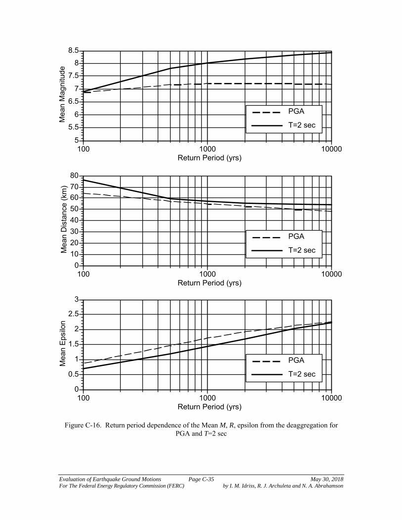
Evaluation of Earthquake Ground Motions Page C-35 May 30, 2018 For The Federal Energy Regulatory Commission (FERC) by I. M. Idriss, R. J. Archuleta and N. A. Abrahamson
Figure C-16. Return period dependence of the Mean M, R, epsilon from the deaggregation for PGA and T=2 sec
5
5.5
6
6.5
7
7.5
8
8.5
100 1000 10000
Me
an
Ma
gn
itud
e
Return Period (yrs)
PGA
T=2 sec
0
10
20
30
40
50
60
70
80
100 1000 10000
Mea
n D
ista
nce
(km
)
Return Period (yrs)
PGA
T=2 sec
0
0.5
1
1.5
2
2.5
3
100 1000 10000
Me
an
Ep
silo
n
Return Period (yrs)
PGA
T=2 sec

Evaluation of Earthquake Ground Motions Page C-36 May 30, 2018 For The Federal Energy Regulatory Commission (FERC) by I. M. Idriss, R. J. Archuleta and N. A. Abrahamson
Figure C-17. Expected spectra for scenario earthquakes for the UHS at T=0.2 sec and T=2.0 sec.
0
0.1
0.2
0.3
0.4
0.5
0.6
0.7
0.8
0.9
1
0.01 0.1 1 10
Spe
ctra
l Acc
eler
atio
n (g
)
Period (sec)
2000 Yr UHS
Juan de Fuca Scenario (T=0.2)
Cascadia Scenario T=2.0)

Evaluation of Earthquake Ground Motions Page C-37 May 30, 2018 For The Federal Energy Regulatory Commission (FERC) by I. M. Idriss, R. J. Archuleta and N. A. Abrahamson
Figure C-18. Example of broadening the expected spectra for scenario earthquakes into a small set of design spectra.
0
0.2
0.4
0.6
0.8
1
1.2
0.01 0.1 1 10
Spe
ctra
l Acc
eler
atio
n (g
)
Period (sec)
2000 Yr UHS
Juan de Fuca Scenario (T=0.2)
Cascadia Scenario T=2.0)
Design Spectra 1
Design Spectra 2

Evaluation of Earthquake Ground Motions Page D-1 May 30, 2018 For The Federal Energy Regulatory Commission (FERC) by I. M. Idriss, R. J. Archuleta and N. A. Abrahamson
APPENDIX D EARTHQUAKE GROUND MOTIONS MODELS
D.1 GENERAL Earthquake ground motions models (GMMs), which historically had been designated as attenuation relationships, are needed to calculate the estimated levels of shaking at a rock outcrop at the site of interest. These GMMs are needed for a deterministic seismic hazard analysis (DSHA) as well as for a probabilistic seismic hazard analysis (PSHA). Many GMMs have been published over the past several decades and more GMMs will be published in the coming years. The increasing number of recordings during earthquakes occurring in various tectonic regimes (shallow crustal earthquakes in active tectonic regions, shallow crustal earthquakes in stable continental regions, or subduction zone earthquakes) have made it possible to derive empirically-based earthquake ground motion models. Improvements and refinements in computational seismology (see Appendix E) have also contributed to augmenting the recorded data for assessing the influence of key physical parameters that are not sufficiently covered by the available recordings. Accordingly, instead of designating "acceptable" GMMs, the acceptability of the selected models will be evaluated on a case by case basis. The general attributes to be considered in such an evaluation include: 1. The GMM has been published in a peer-reviewed publication such as Spectra, the Journal of
the Earthquake Engineering Research Institute (EERI), the Bulletin of the Seismological Society of America, ASCE Journal of Geotechnical and Geoenvironmental Engineering … etc.
Exceptions may be made, if warranted by the documentations provided by the owner of the facility.
2. The GMM is applicable to the tectonic regime (or regimes) relevant to the site under considerations.
3. The GMM is applicable to the condition relevant to the location of the structure (e.g.,
embankment) under consideration. For example, if the structure is located on the hanging wall of a crustal source in West North America (WNA), only three of the NGA West2 GMMs explicitly account for the effects of the hanging wall; accordingly, only these three GMMs are to be used in that case.
4. The values of all the pertinent parameters used in the GMM. For example, the list of parameters
used in the NGA West2 and the definition of each are included in Table D-1.
5. To the extent possible, more than one GMM should be used to estimate the earthquake ground motions generated from a specific seismic source.
6. The earthquake ground motions estimated by one or more GMM may be required to be checked
against available relevant recorded data to examine the reasonableness of the results calculated using the selected GMM.

Evaluation of Earthquake Ground Motions Page D-2 May 30, 2018 For The Federal Energy Regulatory Commission (FERC) by I. M. Idriss, R. J. Archuleta and N. A. Abrahamson
D.2 THE NEW GENERATION ATTENUATION (NGA) PROJECTS Because of the extensive work that has taken place as part of the NGA Projects over the past 14 years, a brief summary of these projects is included in this section. The NGA West1 (considering only earthquake ground motions recorded during crustal events) Project was initiated in 2004 and completed in 2008 at the Pacific Engineering Earthquake Research Center (PEER) headquartered at the University of California at Berkeley. The resulting models were published in the 2008 February issue of Spectra, the Technical Journal of the Earthquake Engineering Research Institute (EERI). Since then, three additional projects have been added:
1. NGA West 2: This project was an augmentation of the NGA West1 project and included a large increase in the number of recordings obtained during earthquakes occurring on crustal sources in the magnitude range of 3 to 7.9. The attenuation relationships derived as part of this project were published in the 2014 August issue of Spectra, the technical journal of the Earthquake Engineering Research Institute.
2. NGA East: The scope of this project was to develop a new ground motion characterization model for the Central and Eastern North-American (CENA) region. This project also involved collecting recorded data from a very large number of earthquakes. However, except for a handful (4) of recordings, the available recordings had been obtained during earthquakes with magnitudes less than 6. Therefore, more reliance was placed on simulations for deriving attenuation relationships. The results are available in a number of PEER reports available at http://peer.berkeley.edu/.
3. NGA Subduction: This project is ongoing and results are expected in 2018/2019. Finally, in addition to reports, Flatfiles, spreadsheets etc., relevant to all the NGA Projects can be accessed at http://peer.berkeley.edu/. D.3 GROUND MOTION MODELS BEING USED BY USGS The paper by Rezaeian et al. (2015)1 lists the earthquake ground motion models being used since 2014 by USGS in preparing the seismic hazard maps. It is expected that USGS will be eliminating a number of models listed in Rezaeian et al. (2015) and adding new GMMs, when such models become available and have been appropriately peer-reviewed.
1 Rezaeian, Sanaz, Petersen, Mark D. and Moschetti, Morgan P. (2015). "Ground Motion Models Used in the 2014 U.S. National Seismic Hazard Maps", Earthquake Spectra, Vol. 31, No. S1, December, pp S59 – S84.

Evaluation of Earthquake Ground Motions Page D-3 May 30, 2018 For The Federal Energy Regulatory Commission (FERC) by I. M. Idriss, R. J. Archuleta and N. A. Abrahamson
Table D-1 Definition of parameters and values used in NGA West2 equations to calculate spectral values for crustal event
Symbol Description
Mw Moment magnitude RRUP Closest distance to rupture surface (km). See sketches a, b and c below for illustration.
RJB Closest distance to surface projection of co-seismic rupture (km). See Figures a, b and c for illustration
RX Horizontal distance from top of rupture measured perpendicular to fault strike (km). See sketches a, b and c below for illustration
VS30 The average shear-wave velocity (m/s) over a subsurface depth of 30 m
FRV Reverse-faulting factor: 0 for strike slip, normal, normal-oblique; 1 for reverse, reverse-oblique and thrust
FNM Normal-faulting factor: 0 for strike slip, reverse, reverse-oblique, thrust and normal-oblique; 1 for normal
FHW Hanging-wall factor: 1 for site on down-dip side of top of rupture; 0 otherwise Dip Average dip of rupture plane (degrees) ZTOR Depth to top of seismic rupture (km) ZHYP Hypo-central depth from the earthquake Z1.0 Depth to Vs=1 km/sec (km) Z2.5 Depth to Vs=2.5 km/sec (km) W Fault rupture width (km)

Evaluation of Earthquake Ground Motions Page E-1 May 30, 2018 For The Federal Energy Regulatory Commission (FERC) by I. M. Idriss, R. J. Archuleta and N. A. Abrahamson
APPENDIX E ANALYTICAL SIMULATIONS TO GENERATE ACCELEROGRAMS
AT A ROCK SITE E.1 INTRODUCTION Different approaches can be used to simulate ground motion from an earthquake source. Some of these approaches are summarized below as examples, but not endorsement, of various methods being currently used. While the approaches can differ, they have in common certain elements that are critical in the evaluation of their applicability. It is also important to note that the synthetic time histories of ground motion are computed for a rock outcrop, i.e., analytical models are computed using linear wave propagation and includes the Earth’s free surface. Treatment of the local site condition is a complicated subject in its own right and is specific to the individual case. The basic axiom of an analytical model is that an earthquake represents the release of elastic energy by slip occurring over some fault plane with finite area in the Earth. The earthquake initiates at the hypocenter, the point on the fault where the slip first occurs and from which the first elastic waves are emitted. As the rupture spreads over the fault, other points on the fault will slip and radiate elastic waves. The elastic waves propagate through a complex earth structure that can scatter and attenuate the waves. The final ground motion that is recorded is a convolution of the earthquake source and the path effects. Consequently, both the source and the path must be fully described to understand the ground motion that has been computed. E.2 COMPONENTS OF AN ANALYTICAL MODEL The essential components that should be described for any analytical model are: 1. Geometrical description of fault and stations for which ground motion will be computed
a. Length of fault b. Width of fault c. Dip of fault d. Strike of the fault (measured clockwise from North, Aki and Richards convention) e. Geometry of fault within the earth, e.g., depth of the shallowest part of the fault, depth
of the deepest part of the fault. f. Hypocenter coordinates: latitude, longitude and depth. g. Geometry of the site relative to the geometry of the fault; any measure of distance
between the fault and site must be specified if this distance measure is used for other purposes, e.g., empirical regression formulas. latitude, longitude and elevation must be specified for each site.

Evaluation of Earthquake Ground Motions Page E-2 May 30, 2018 For The Federal Energy Regulatory Commission (FERC) by I. M. Idriss, R. J. Archuleta and N. A. Abrahamson
2. Gross parameters of the earthquake
a. Seismic moment (All magnitudes must be converted to moment magnitude; magnitude and seismic moment must be internally consistent. The precise formula for converting magnitude to seismic moment and vice versa must be specified, e.g.,
210.7
3 oM Log M where Mo is seismic moment in dyne-cm (Hanks and
Kanamori, 1979))
b. Magnitude of slip specified for each point on the fault where is the coordinate
along strike and is the coordinate along the dip. The basis for deciding on a spatial
distribution of slip, e.g., a distribution similar to a previous earthquake, and the basis for deciding on the amplitude of slip, e.g., scaled slip from previous earthquake, must be specified. If the fault is a plane, this description should be a 2 by 2 matrix of slip values with each slip value given a coordinate on the fault.
c. Slip direction for each point on the fault: rake angle. If the slip value is partitioned into two components: slip along strike and slip along the dip direction, the rake angle is superfluous.
d. Slip time function for every point on the fault or a proxy for the slip time function, e.g., Fourier amplitude spectrum.
e. Rupture time. For each point on the fault, the time at which that points first begins to slip must be specified. The hypocenter has a rupture time of zero.
3. Gross parameters of the Earth structure everywhere in the body of the medium
a. Velocity of elastic waves (P and S) b. Density c. Attenuation by use of the seismic quality factor Q; the quality factor may be frequency
dependent. If that is the case, its frequency dependence must be specified. 4. Site Characterization—Rock
a. P- and S-wave velocity and attenuation, Q(f) at the site b. Linear response c. Spatially non-uniform material properties if they exist.
5. Full description of the method of computing Green’s functions must include:
a. Method for computing the Green's functions must be described including details such as the exact time function used for the impulse source, the time step, numerical damping, low-pass and/or high-pass filters, etc.
b. A precise description of the velocity structure must be given (see Item 3) as well as the frequency bandwidth for which the Green's functions are computed.
c. If empirical Green’s functions are used, their applicable frequency bandwidth must be specified. The location of the source must be specified. Any scaling between the original source and that used for the convolution must also be specified.
6. Full description of how the source is convolved with the Green's functions.
a. Specify the exact locations of the slip functions on the fault, e.g., rectangular grid, non-uniformly, and how the slip functions are convolved.
b. Explain how each of the parameters are used in the convolution is specified on the fault.

Evaluation of Earthquake Ground Motions Page E-3 May 30, 2018 For The Federal Energy Regulatory Commission (FERC) by I. M. Idriss, R. J. Archuleta and N. A. Abrahamson
c. Are there further refinements to slip functions and Green's functions before convolution? For example, are either the Green's functions or the slip functions or both interpolated to a finer spatial scale? Is there filtering applied?
7. Documentation that the analytical model computes ground motion consistent with ground
motion from recorded earthquakes. a. There must be some measure of the misfit between the recorded ground motion and
the computed ground motion. For example, it is customary to compute bias and standard error for different periods of the response spectrum, e.g., Hartzell et al. (1999), Goulet et al. (2015).
b. In comparing recorded ground motion with that from an analytical method, there should be a minimum of five stations with maximum (360˚ ideally) azimuthal coverage of the source.
c. If a preexisting method is being used for analytical computation of ground motion, any previous validation studies should be cited provided the method has not changed since the validation studies were originally performed.
E.3 AVAILABLE ANALYTICAL MODELS There are a variety of different models that have been used to calculate earthquake ground motions. The methods are continually evolving, especially those that include the finite extent of the fault and are broadband [frequencies from 0–20 Hz, e.g., see Goulet et al. (2015)] and associated papers in the same publication). Calculating broadband time histories often involves computing broadband synthetics by stitching low-frequency (f ≤ 1.0 Hz) synthetics with high-frequency Green's functions, either synthetic or empirical (e.g., Hutchings, 1994; Pitarka et al., 2000; Archuleta et al., 2003; Kamae et al., 2005; Frankel, 2009). In many approaches the Green's function is simply 1/R with an attenuation; however, the source itself is stochastic (e.g., Boore, 1983, 2003; Graves and Pitarka, 2010). Some approaches are for point sources, i.e., the site is far from the source so that any timing issues related to the physical dimensions of the source are small (i.e., 2
mind R , in
which d is the maximum distance from the hypocenter to any point on the fault, R is the hypocentral distance to the site, and min is the minimum wavelength recorded). Atkinson and Somerville (1994) discuss two different approaches, a stochastic approach (Boore, 1983) and the ray theory approach (Somerville et al., 1991), for simulating ground motions from point sources as applied to earthquakes in the eastern US. For spectral acceleration, the standard error of the estimation for both methods is on the order of 2 to 2.5. Atkinson and Boore (1998) provide a more detailed analysis of different spectral models as applied to eastern US earthquakes. This has been a typical standard error as well for analytical models that include finite faulting for broadband ground motion (e.g., Kamae et al., 1998; Hartzell et al., 1999; Pitarka et al., 2000; Mai and Beroza, 2003, Archuleta et al., 2003, and broadband papers in Seismological Research Letters, v. 86 (1), 2015). Rather than endorse any particular modeling effort, it is important to understand how the different elements of the model are computed and then combined to produce a broadband synthetic ground motion (Spudich and Archuleta, 1987). Selecting a source model, i.e., the slip rate function everywhere on the fault and the rupture time for each point depends on the investigator. Naturally, there has to be justification for the source model (e.g., Andrews, 1980; Boatwright, 1988; Herrero and Bernard, 1994; Mai and Beroza, 2002; Oglesby and Day, 2002; Lavallée and Archuleta, 2003, Crempien and Archuleta, 2015). However, with analytical models it is important to consider multiple source descriptions in order to understand the range of ground motions that may occur

Evaluation of Earthquake Ground Motions Page E-4 May 30, 2018 For The Federal Energy Regulatory Commission (FERC) by I. M. Idriss, R. J. Archuleta and N. A. Abrahamson
from a scenario earthquake (O’Connell et al., 2001; Hartzell et al., 2002; Archuleta et al., 2003; Day, 2003; Mai and Beroza, 2003; Liu et al., 2006; Crempien and Archuleta, 2015). A real difficulty in broadband synthetics is the estimation of the appropriate Green's function. Computing full waveform Green's functions in 1-D layered models is standard practice (e.g., Olson et al., 1984; Zhu and Rivera, 2001). The 1-D Green's functions are easily computed up to frequencies of 20 Hz including Q. With the development of finite difference and finite element codes it is possible to compute accurately Green's functions in 2D and 3D Earth models (e.g., Olsen et al., 1995; Graves, 1996; Day, 1982, 2001, 2005; Moczo et al., 2001, Ma et al., 2004). However, such computations are generally limited to computing ground motions for frequencies less than 1.0 Hz. If the numerical 2D and 3D Green's functions are to be extended to higher frequencies, the investigator has to find a way to stitch together the different passbands (e.g., Kamae et al., 1998; Hartzell et al., 1999; Pitarka et al., 2000; Mai and Beroza, 2003; Liu et al., 2006). Clearly, the most straightforward approach is to use events recorded at the site as empirical Green's functions following the seminal paper of Hartzell (1978). This technique has been widely used, for example, Irikura, (1983), Joyner and Boore (1986), Dan et al. (1990), Wennerberg (1990), Somerville et al. (1991), Hutchings (1994), Irikura and Kamae (1994), Tumarkin and Archuleta (1994), Tumarkin et al. (1994), Ordaz et al. (1995), Jarpe and Kasameyer (1996), Archuleta et al. (2003), Miyake et al. (2003). This has the obvious limitation that the site must have recorded an earthquake from the source zone of the earthquake to be modeled. E.4 CONCLUDING REMARKS Before applying an analytical model, the analytical model must be validated. The standard approach is to model a well-recorded earthquake. The synthetic time series is compared both in the time domain and spectral domain with the recorded data. Examples of such comparisons can be found in Somerville et al. (1991), Hartzell et al. (1999), Archuleta et al. (2003), Mai and Beroza (2003) and Goulet et al. (2015).
Evaluation of Earthquake Ground Motions Page F-1 May 30, 2018 For The Federal Energy Regulatory Commission (FERC) by I. M. Idriss, R. J. Archuleta and N. A. Abrahamson
APPENDIX F SELECTION OF ACCELEROGRAMS FOR
SEISMIC ANALYSIS PURPOSES F.1 GENERAL The most widely used procedures to obtain accelerograms (i.e., acceleration time histories or time series) for use in a seismic analysis, once a target spectrum is defined, are:
a. Utilization of motions previously recorded at rock sites during similar magnitude earthquakes and at distances comparable to those under consideration. This procedure may be described as "direct use" of recorded motions.
b. Selection of motions recorded during similar magnitude earthquakes and then adjusting
each accelerogram so that its spectral ordinates are essentially equal to those of the target spectrum. This procedure may be described as "use of constructed spectrum-compatible" accelerograms.
These procedures are summarized below. F.2 DIRECT USE OF RECORDED MOTIONS Time histories recorded during several earthquakes are available from several web sites including COSMOS (http://www.cosmos-eq.org/), USGS, the California Geological Survey, and the Pacific Earthquake Engineering Research center (http://ngawest2.berkeley.edu/). The following issues are important to consider when using this procedure:
The accelerograms should be selected from those recorded at rock sites (VS30 ≥ 600 m/sec); the USGS considers a "generic rock site" as having a VS30 = 760 m/sec.
The accelerograms should be selected from those recorded during earthquakes having magnitudes as close to the magnitude of the event that controlled the target spectrum; variations of up ±¼ magnitude may be considered.
The distance should also as close to the distance obtained for the event controlling the target spectrum; if R is the latter distance, then distances for the "seed" time histories can range from about ½R to about 1½R.
The selected time histories can be scaled, but that scaling factors should be limited to no more than 2.
It is important that the average of the spectra of the selected time histories (after scaling) be as close as possible to the target spectrum, especially over the "critical" frequency range.
When using recorded time histories directly as recorded, or with minor modifications, it is recommended that at least seven time histories, and possibly as many as nine or more, be used in the analyses to represent each target spectrum.

Evaluation of Earthquake Ground Motions Page F-2 May 30, 2018 For The Federal Energy Regulatory Commission (FERC) by I. M. Idriss, R. J. Archuleta and N. A. Abrahamson
F.3 CONSTRUCTION OF SPECTRUM-COMPATIBLE ACCELEROGRAMS This procedure also starts with selecting recorded time histories from the sources listed in Section F.2 above. The following issues are important to consider when using this procedure:
The site conditions can be less restrictive than those for the procedure listed in Section F.2. The accelerograms (typically referred to as "seed" time histories) can be selected from those recorded not only at rock sites, but also at relatively stiff sites. It is suggested that sites with VS30 ≥ 400 m/sec be considered for this purpose.
The accelerograms should be selected from those recorded during earthquakes having magnitudes as close to the magnitude of the event that controlled the target spectrum; variations of up ±¼ magnitude may be considered.
The distance should also as close to the distance obtained for the event controlling the target spectrum; if R is the latter distance, then distances for the "seed" time histories can range from about ½R to about 1½R.
The selected time histories can be scaled, but that scaling factors can be less restrictive than for the procedure listed in Section F.2. Nevertheless, the factor for this procedure is best limited to no more than 3.
To obtain the spectrum-compatible time history, the "seed" accelerogram is modified, in either the time domain or in the frequency domain, so that the its spectral ordinates are essentially equal to those of the target spectrum. The frequency domain procedure is described in Silva and Lee (1987), and the time domain solution is described in Lilhanand and Tseng (1988). For many projects, three "seed" time histories have been selected for each target spectrum under consideration. It is recommended that considerations be given to requiring more (say seven "seed" time histories) for each target spectrum. F.4 PLOTS The following plots should be provided for each accelerogram:
Time series of acceleration, velocity and displacement; Acceleration spectrum (pseudo-absolute acceleration versus period) together with the
target spectrum; Husid plot to assess duration (based on 5% to 95% of Arias intensity); and Fourier amplitude versus frequency (log-log scale).
Note that these plots should be provided for each:
The scaled accelerogram (if it is to be used directly in the analysis). The "seed" time history. The spectrum-compatible time history.