Engineering Economics (Cost Function)

Engineering Economics(Cost Function)

Concepts of Cost

• The term “Cost” is used in many sense and hencehas many concepts. All these need to be properlyand clearly understood.

Real Costs

• real cost included the following two basic elements:

• Exertions Of All Kinds Of Labour;

• Waiting And Sacrifices Required For Saving TheCapital It Is More A Psychological Concept AndCannot Be Measured.

• Therefore, It Is Not Applied In Actual Practice.

Real Costs

Economic Costs

• The total expenses incurred by a firm in

producing a commodity are generally

termed as its economic costs. Economic

costs are generally referred to as production

costs as well.

The Total Economic Costs Include

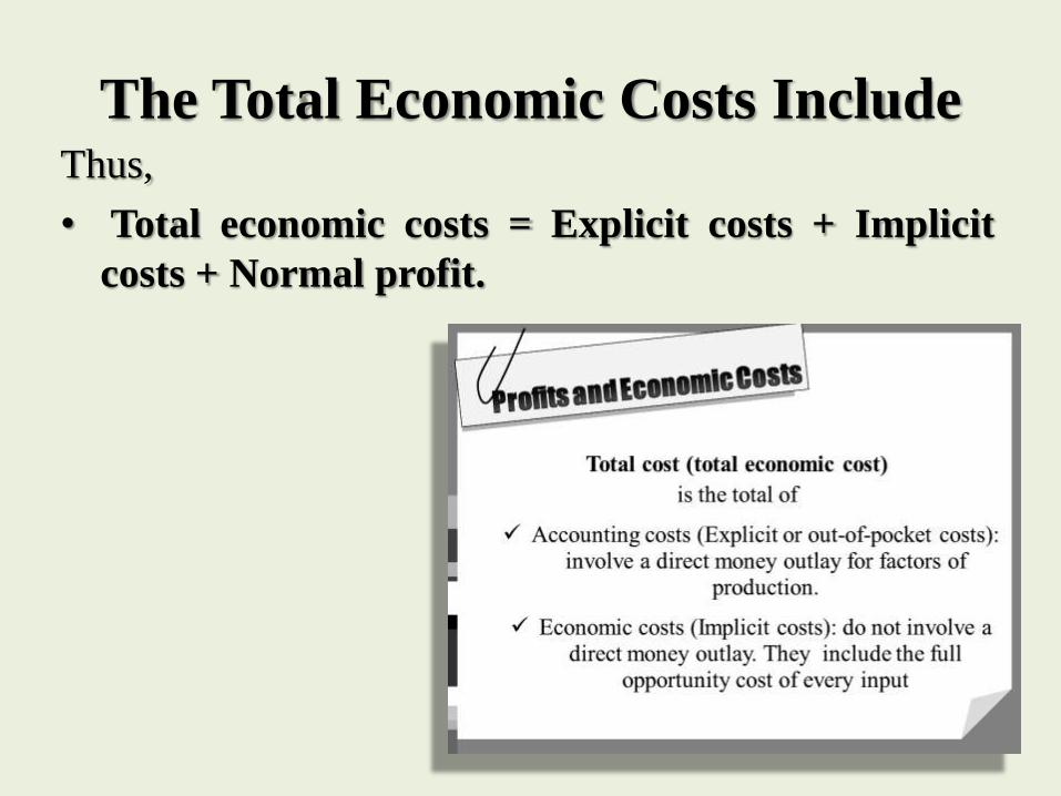
The Total Economic Costs IncludeThus,

• Total economic costs = Explicit costs + Implicit

costs + Normal profit.

The Total Economic Costs Include

• Generally economic costs include the

following:

• Cost of the raw materials, wages, interest,

rent, management costs, depreciation of

capital equipment, expenditure on publicity

and advertisements, transport costs, costs of

the producer’s own resources, normal profit,

other expenses etc.

Total Economic Costs

Opportunity Cost

Opportunity Cost

• The concept of opportunity cost occupies a very importantplace in modern economic analysis.

• Factors of production are scarce in relation to wants.

• When a factor is used in the production of a particularcommodity, the society has to forgo other goods which thisfactor could have produced.

• This gave birth to the notion of opportunity cost in economics.

• Suppose a particular kind of steel is used in manufacturing war-goods, it clearly implies that the society has to give up theamount of utensils that could have been produced with thehelp of this steel.

• Hence we can say that the opportunity cost of producing war-goods is the amount of utensils forgone.

• Opportunity cost is the cost of the next-best alternative that hasbeen forgone.

Opportunity Cost

Opportunity Cost

• From the meaning of opportunity cost twoimportant points emerge:

• (i) The opportunity cost of anything is onlythe next-best alternative foregone and notany other alternative.

• (ii) The opportunity cost of a good should beviewed as the next-best alternative good thatcould be produced with the same value ofthe factors which are more or less the same.

Opportunity Cost

• The concept of opportunity cost can better

be explained with the help of an illustration.

Suppose a price of land can be used for

growing wheat or rice. If the land is used for

growing rice, it is not available for growing

wheat.

Opportunity Cost

• Therefore the opportunity cost for rice is the wheat

crop foregone. This is illustrated with the help of the

following diagram:

Opportunity CostSuppose the farmer, using a piece of land can produce either 50 quintals

(ON) of rice or 40 quintals (OM) of wheat.

• If the farmer produces 50 quintals of rice (ON), he cannot produce wheat.

• Therefore the opportunity cost of 50 quintals (ON) of rice is 40 quintals

(OM) of wheat.

• The farmer can also produce any combination of the two crops on the

production possibility curve MN.

• Let us assume that the farmer is operating at point A on the production

possibility curve where he produces OD amount of rice and OC amount

of wheat.

• Now he decides to operate at point B on the production possibility curve.

• Here he has to reduce the production of wheat from OC to OE in order to

increase the production of rice from OD to OF.

• It means the opportunity cost of DF amount of rice is the CE amount of wheat.

• Thus, opportunity cost for a commodity is the amount of other next-best

goods which have to be given up in order to produce additional amount of that

commodity.

Opportunity Cost

Applications of Opportunity Cost


• The concept of opportunity cost has been widely used by

modern economists in various fields. The main

• applications of the concept of opportunity cost are as follows –

• (i) Determination of factor prices - The factors of

production need to be paid a price that is at least equal to

what they command for alternative uses. If the factor price is

less than factor’s opportunity cost, the factor will quit and get

employed in the better-paying alternative.

• (ii) Determination of economic rent - The concept of

opportunity cost is widely used by modern economists in

the determination of economic rent. According to them

economic rent is equal to the factor’s actual earning minus

its opportunity cost (or transfer earnings).


(iii) Decisions regarding consumption pattern - The concept of

opportunity cost suggests that with given money income, if a

consumer chooses to have more of one thing, he has to have

more of one thing, he has to have less of the other. He cannot

increase the consumption of all the goods simultaneously.

(iv) Decisions regarding production plan - With given resources

and given technology if a producer decides to produce greater

amount of one commodity, he has to sacrifice some amount of

another commodity. Thus on the basis of opportunity costs a firm

makes decisions regarding its production plan.

(v) Decisions regarding national priorities - With given resources at

its command a country has to plan the production of various

commodities. The decision will depend on national priorities

based on opportunity costs.

Cost-Function

The functional relationship between cost and quantityproduced is termed as cost function.

C = f(Q )

• Here,

• C = Production-cost

• Q x = Quantity produced of x goods

• Cost-function of a firm depends on two things:

• (i) Production-function, And

• (ii) The Prices Of The Factors Of Production.

• Higher the output of a firm, higher would be the production-cost. That is why it is said that the cost of productiondepends on the quantum of output.

Short Run Cost Function

Economists have treated cost as a function of output both

in short run and long run.

Long Run Cost Function

Time Element And Cost

• Time element has an important place in the analysis of cost of production. In the

theory of supply we usually take three kinds of time-period. They are:

• (i) Very Short-period - Very short-period is defined as the period of time

which is so short that the output cannot be adjusted with the change in demand.

In this period, the supply of a commodity is limited to its stock, hence during this

period supply remains fixed.

• (ii) Short Period - Short period is defined as the period of time during which

production can be varied only by changing the quantities of variable factors

and not of fixed factors; Land, factory building, heavy capital equipment,

services of management of high category are some of the factors that cannot be

varied in a short period. That is why they are called fixed factors.

• There are some factor-inputs that can be varied as and when required. They are

called variable factors. For instance, power, fuel, labour, raw materials, etc. are the

examples of variable factor inputs.

• (iii) Long Period - Long period is defined as the period which is long enough

for the inputs of all factors of production to be varied. In this period no factor

is fixed, but all are variable factors.

Time Element And Cost

Short-Run Costs

• In the short-run, a firm employs two types of factors : fixed factors and

variable factors. Costs are also of two types : fixed costs and variable costs.

• (i) Fixed Costs - Fixed costs (also known as supplementary costs or

overhead costs) are the costs that do not vary with the output. These are

the expenses incurred on the fixed factors of production.

• Examples: Rent; interest; insurance premium; salaries of permanent

employees, etc.

• (ii) Variable Costs - Variable costs (or prime costs) are the costs that

vary directly with the output. These are the expenses incurred on the

variable factors of production.

• Examples: Expenses on raw materials, power and fuel; wages of daily

labourers, etc.

Short-Run Costs

Distinctions between Fixed Costs

and Variable Costs

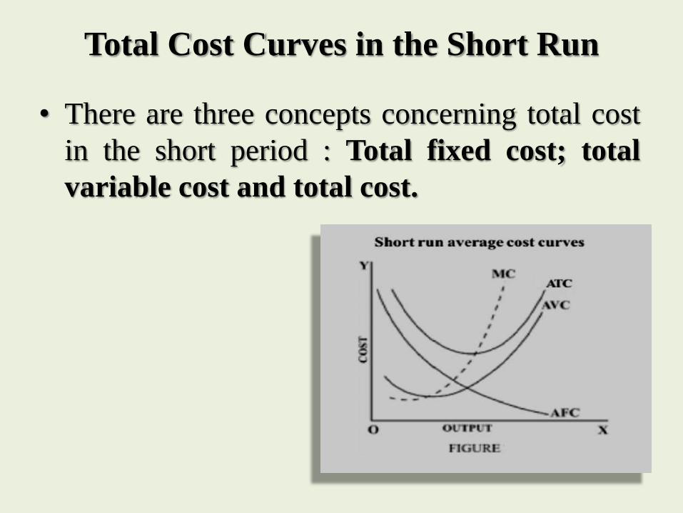
Total Cost Curves in the Short Run

• There are three concepts concerning total cost

in the short period : Total fixed cost; total

variable cost and total cost.


(i) Total Fixed Cost (TFC) – Total Fixed Costs are those costs thatdo not vary with the output. They continue to be the same even ifoutput is zero or 1 unit or 10 lakhs units. Thus, they are totallyunaffected by the changes in the rate of outputs. These costs are alsooften referred to as supplementary costs or overhead costs orunavoidable costs.

Examples of fixed costs are :

(i) Initial establishment expenses,

(ii) Rent of the factory,

(iii) Expenses on maintenance of Machinery;

(iv) Wages and salaries of the permanent staff,

(v) Interests on bonds,

(vi) Insurance premium.

• TFC = quantities of the fixed productive service x factorprice.

Total Fixed Cost (TFC)


• TFC = quantities of the fixed productive service

x factor price.

• Total fixed cost of a firm is illustrated in the

following table and diagram :

TFC curve is a horizontal line parallel to the x-axis which

explains total fixed cost remains the same at all levels of

output.

Total Variable Cost (TVC)

(ii) Total Variable Cost (TVC) – The costs thatvary directly with the output and rises as moreis produced and declines as less is produced,are called total variable costs. They are alsoreferred to as prime costs or special costs ordirect costs or avoidable costs. Examples ofvariable costs are : (i) wages of temporarylabourers; (ii) raw materials; (iii) fuel; (iv)electric power, etc.

• TVC = quantities of the variable factor service ×factor price.


• Total Variable Cost is illustrated in the following

table and diagram :


• TVC curve starts from the origin, up to a

certain range remains concave from below

and then becomes convex. It shows that in the

beginning, total variable cost rises at a

diminishing rate and thereafter, it rises at

increasing rates.

Total Cost

(iii) Total Cost – Total Cost means the total cost of producing any given amount of

output. When we add total fixed and total variable costs at different levels of

output, we get the corresponding total costs.

• Thus, TC = TFC + TVC

• Since, fixed costs are constant and variable costs necessarily rise as output rises,

total costs also rise with the output or, to put the point more technically, TC is a

function of total product and varies directly with it : TC = f(q).

• TC (Total Cost) curve can be obtained by adding TFC and TVC curves

vertically at each point.

• Again, since the total fixed cost, by definition remains constant, the changes in the

total costs are entirely due to the changes in total variable costs. In other words, the

rate of increase of total cost is the same as of total variable cost, as one of the

two components of total cost remains constant. TC and TVC curves, therefore,

have the similar shapes, the only difference is that TVC curve starts from

origin (O) while TC curve starts above the origin. Initially TC will include the

amount of TFC and hence it starts from the positive intercept.

Total Cost

The relationship between these three – TFC, TVC

and TC is illustrated in the following table and

diagram :

TFC, TVC and TC curve

Unit Cost Curves in Short-Run


• The short-run unit cost curves are : Average Fixed Cost(AFC) curve; Average Variable Cost (AVC) curve; AverageTotal Cost (ATC) or Average Cost (AC) curve; andMarginal Cost (MC) curve. For price and outputdetermination, per unit cost curves are more useful than thetotal costs just discussed.

• (i) Average Fixed Cost (AFC) – Average fixed cost can beobtained by dividing total fixed cost (TFC) by thequantity of output (Q),

• AFC = TFC/Q

• Since total fixed costs remain the same, as output rises,average fixed cost diminishes but never becomes zero.

Average Fixed Cost (AFC)


Features of AFC –

• (i) As output rises, the average fixed cost (AFC) goes ondeclining. The AFC curve is, therefore, a downward slopingcurve,

• (ii) As output approaches zero, average fixed costapproaches infinity, but AFC curve never touches the y-axis. On the other hand, as output reaches very high levels,average fixed cost approaches zero, but it never becomeszero, it always remains positive. Hence the AFC curvenever touches the x-axis. Thus it follows that AFC curvenever touches either of the axis. Actually AFC curve takesthe shape of rectangular hyperbola which shows that thearea under the curve (i.e. total fixed cost) always remainsthe same.

AFC is illustrated in the following table

and diagram.

Average Variable Cost (AVC)

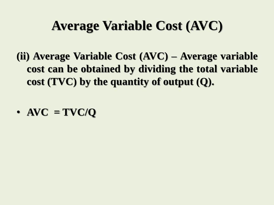
(ii) Average Variable Cost (AVC) – Average variable

cost can be obtained by dividing the total variable

cost (TVC) by the quantity of output (Q).

• AVC = TVC/Q


• As output rises, the AVC curve first falls, reaches a

minimum and then begins to rise.

• Thus, AVC curve has a U-shape.

Average Total Cost (ATC) or

Average Cost (AC)

(iii) Average Total Cost (ATC) or Average Cost (AC) –Average total cost (ATC) is obtained by dividing thetotal cost (TC) by the quantity of output (Q). Thus,average cost (AC) is the per unit cost of production of acommodity. Or, alternatively, it can also be obtained byadding average fixed cost (AFC) and average variablecost (AVC).

• ATC = TC/Q

• Or, ATC = AFC + AVC

• Diagrammatically the vertical summation of average fixedcost and average variable cost curves gives us the averagetotal cost curve. The ATC curve is also a U-shaped curve.

Average Cost (AC)

Marginal Cost (MC)

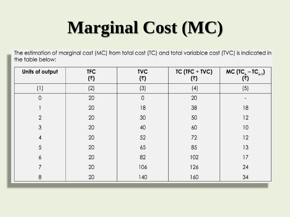
(iv) Marginal Cost (MC) — Marginal cost is theincrease in total cost resulting from one unitincrease in output. In short, it may be calledincremental cost. Thus,

• MC = dTC/dQ

• Or, M Cn = TCn - TC n-1

• Here, MC = Marginal Cost

• TCn = Total Cost of n units of output

• TC n-1 = Total Cost of n-1 units of output

Marginal Cost (MC)

Marginal Cost (MC)

• Since a change in total cost is caused only by a

change in total variable cost, marginal cost may

also be defined as the increase in total variable

cost resulting from one unit increase of output.

Thus, marginal cost has nothing to do with the fixed

costs.

• Suppose the total variable cost of 4 units of output is `

52 and the total variable cost of 3 units is ` 40, then

the marginal cost will be ` 12 (52-40).

Marginal Cost (MC)

Relationship between AC and MC

• Average Cost is simply the total cost (TC)

divided by the number of units produced

(Q) or it is the cost per unit.

• On the other hand, marginal cost is defined as

the increment of total cost that comes from

producing an increment of one unit of output.

The relationship between AC and MC is illustrated

in the following table and diagram below:

The relationship between AC and MC

Long - Run Cost

Long - Run Cost

• In the long-run, a firm can vary its scale of plant asand when it requires. All factor-inputs are thusvariable in this period.

• Therefore, there are no fixed cost curves in thelong-run.

• All cost curves in the long-run are basically variablecost curves. Here we find the following cost curves :

• Long-run Total Cost (LTC) curve;

• Long-run Average Cost (LAC) curve; and

• Long-run Marginal Cost (LMC) curve.

Long-run Average Cost Curve:

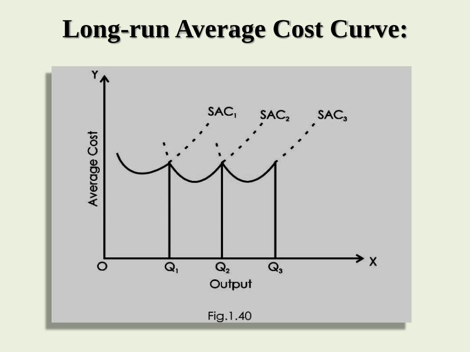
•A firm has a fixed scale of plant in the short-run.

• A short-run Average Cost (SAC) curve corresponds to a particular scaleof plant.

• In the short-run, the firm can operate only on a particular scale of plant.

• In the long-run a firm can choose among possible sizes of plant or it canmove from one scale of plant to the other scale of plant.

• The choosing of the scale of plant is depends on the quantity of outputthat a firm wants to produce.

• A firm would like to produce a given level of output at the minimumpossible cost.

• The firm would like to build its scale of plant in accordance with thequantity of output in such a way that it can minimise its average cost.

• Suppose a firm can have three possible scales of plant which are shown bySAC 1 , SAC 2 and SAC 3 curves in the diagram.

• In the long-run, a firm can choose any scale of plant out of these threeplants.

• The choice of the scale of plant will depend on the quantity of output.

Long-run Average Cost Curve:

Long-run Marginal Cost Curve

Relationship between LAC and LMC

• It should also be noted here that the relationship between LAC

curve and LMC curve is the same as that

Relationship between LAC and

LMC

• between SAC curve and SMC curve. Thus, when

LMC curve lies below the LAC curve, the latter will

be falling and when the LMC curve lies above the

LAC curve, the latter will be rising. And the LMC

curve cuts the LAC curve at its minimum point. LAC

and LMC curves are also U-shaped curves. But they

are flatter than the short-run cost curves.

Why is LAC curve U-shaped?

Economies and Diseconomies of Scale

• We have already said that the U-shape of LAC curve is becauseof returns to scale.

• And returns to scale is the result of economies and diseconomiesof scale.

• With the expansion of the scale of production firms get certainadvantages, these are termed as economies of large scale production.But when the scale of production exceeds a certain limit, it leads todisadvantages or diseconomies of scale to the firms. Thus the firmsget economies and diseconomies of scale with the expansion ofoutput. These are termed as economies and diseconomies of largescale production. Economies refer to the saving in per unit cost asoutput increases. On the other hand, diseconomies refer to thedisserving in the per unit cost as output increases.

• Economies and diseconomies of scale are broadly classified intotwo groups:

• (A) Internal economies and diseconomies

• (B) External economies and diseconomies.

Economies and Diseconomies of Scale

Internal Economies and Diseconomies

• Economies and diseconomies that accrue to a firm out of its internal situation

when its scale increase are termed as internal economies and diseconomies.

Now we shall discuss them in detail.

• Internal Economies

• Internal Economies that accrue to a particular firm with the expansion of its

output and scale are termed is internal economies. Internal economies of a firm

are independent of the action of other firms. They are internal in the sense that they

are limited to a firm when its output increase.

• They are not shared by other firms in the industry. Following are the main types of

internal economies:

• (i) Labour Economies – Division of labour and specialization are possible more

in large-scale operations.

• Different types of workers can specialize and do the job for which they are

more suited. A worker acquires greater skill by devoting his attention to a

particular job. As a result of this quality and speed of work both improve.


(ii) Technical Economies – The main technical economies result

from the indivisibilities. Several capital goods, because of the

strength and weight required, will work only if they are of a

certain minimum size. There is a general principle that as the size

of a capital good is increased, its total output capacity increases far

more rapidly than the cost of making it.

(iii) Marketing Economies – Marketing economies arise from the

large scale purchase of raw materials and other inputs.

• A firm may receive large discounts on the purchase of bigger

volume of raw materials and intermediate goods. Marketing

economies can also be reaped by the firm in its sales promotion

activities. Advertising space (in newspapers and magazines) and

time (on television and radio), and the number of salesmen do

not have to rise proportionately with the sales. Thus per unit

selling cost may also fall with the increase in output.


(iv) Managerial Economies – Managerial economies arise

from specialization of management and mechanisation of

managerial functions. Large firms make possible the division

of managerial tasks. This division of decision—making in

large firms has been found very effective in the increase of the

efficiency of management.

(v) Financial Economies – Large firms can easily raise timely

and cheap finance from banks and other financial

institutions and also from the general public by issue of shares

and debentures.


(vi) Risk-bearing Economies – A large firm can more successfullywithstand the risks of business.

• With the product diversification and by operating in several markets a largefirm can withstand the risk of changing consumer’s tastes and preferences.

(vii) Economies Related to Transport and Storage Costs – Large firms areable to enjoy freight concessions from railways and road transport.Because a large firm uses its own transport means and large vehicles, theper unit transport costs would fall. Similarly, a large firm can also have itsown storage go downs and can save storage costs.

(viii) Other Economies – A large firm may also enjoy some othereconomies with the expansion of its output. Prominent among them areeconomies on conducting research and development activities andeconomies of employee welfare schemes.

• As a result of all these internal economies firm’s long-run average andmarginal cost decline with the increase in output and scale of production.

Internal Diseconomies


• Internal Diseconomies are those disadvantages which are

internal to the firm and accure to the firm when it over

expands its scale of production. The main internal

diseconomies of scale

• are as follows : -

(i) Management Diseconomies and Diseconomies Related to

Division of Labour – These diseconomies occur primarily

because of increasing managerial difficulties with too large

a scale of operations. It becomes difficult for the top

management to exercise control and to bring about proper

coordination.


(ii) Technical Diseconomies – If a firm frequently changes in ittechnologies and uses new technologies and new machines, it mayincrease its costs. After a certain limit, the large size or volume ofthe plant and machinery may also prove disadvantageous.

(iii) Risk-taking Diseconomies – The business cannot be expandedindefinitely because of the

• “principle of increasing risk”. The risk of the firm increasesbecause of reduction in demand, change in fashion and introductionof new substitutes in the market.

(iv) Marketing Diseconomies – A large firm is forced to spend moreon bringing and storing of raw materials and selling of finishedgoods in the distant markets.

(v) Financial Diseconomies – A large firm has to borrow a largeamount of money even at higher rate of interest. It imposes aburden on the financial position of the firm.

Impact of Internal Economies and

Diseconomies on the LAC Curve

• When a firm accrues internal economies with the

expansion of its scale of output, the LAC curve would fall.

And when after a certain point, a firm receives internal

diseconomies with the expansion of its scale of output, the

LAC curve would rise.

• Thus, internal economies causes the LAC to fall and

internal diseconomies cause the LAC to rise.

• Hence the internal economies and diseconomies are

responsible for the U-shaped of the LAC curve. It is shown

in the diagram

Impact of Internal Economies and


External Economies and Diseconomies

• Economies which accrue to the firms as a result ofthe expansion in the output of the whole industryare termed external economies. They are external inthe sense that they accrue to the firms not out of itsinternal situation but from outside it i.e., fromexpansion of the industry.

• Jacob Vinor has defined external economies as‘those which accrue to particular concerns as theresult of expansion of output by the industry as awhole and which are independent of their ownindividual output’.

• Following are the main forms of external economies.


(i) Economies of Localisation/Concentration - When anindustry develops in a particular region, it brings with itall the advantages of localization. All the firms of thisindustry get the following

• main advantages:

• (a) Easy availability of skilled manpower;

• (b) Improvement in transportation and communicationfacilities;

• (c) Availability of banking, insurance and marketingservices;

• (d) Better and adequate sources of energy-electricity andpower;

• (e) Development of ancillary industries.


(ii) Economies of Disintegration/Specialisation – The industry can have

advantages from the economies of specialization when each firm

specializes in different processes necessary for producing a product.

For instance in a cloth industry some firms can specialise in spinning,

others in printing etc. As a result of specialisation all the firms in the

industry would be benefited.

(iii) Economies related to Information Services – Firms in an industry can

jointly set-up facilities for conducting research, publication of trade

journals and experimentation related to industry.

• Thus, besides providing market information, the growth of the industry

may help in discovering and spreading improved technical knowledge.

(iv) Economies of Producer’s Organisation – Firms of an industry may

form an association. Such an association can have their own transport,

own purchase and marketing departments, own research and training

centres. This will help to reduce costs of production to a great extent and

shall be mutually beneficial.

External Diseconomies

• Diseconomies which accrue to the firms as a result of the expansionin the output of the whole industry are termed externaldiseconomies. The main external diseconomies are as follows:

• (i) Increase in input price – When the industry expands, thedemand for factor-inputs increases. As a result the input prices(such as wages, prices of raw materials and machineryequipments, interest rates, transport and communication ratesetc.) shoot up. This causes the cost of production to rise.

• (ii) Pressure on Infrastructure Facilities – Concentration offirms in a particular region creates undue pressure on theinfrastructure facilities – transportation, water, sanitation,power and electricity etc.

• As a result, bottle necks and delays in production process becomefrequent which tend to raise per unit costs.

External Diseconomies

(iii) Diseconomies due to Exhaustible Natural Resources – Diseconomies

may also arise due to exhaustible natural resources. Doubling the

fishing fleet may not lead to a doubling of the catch of fish; or doubling

the plant in mining or on an oil-extraction field may not lead to a doubling

of output.

(iv) Diseconomies of disintegration – When the production of a commodity

is disintegrated among various processes and sub-process, it may prove

disadvantageous after a certain limit. The problem and fault in any one

unit may create limit. The problem and fault in any one unit may create

problem for whole of the industry. Coordination among different concerns

also poses a problem.

• As a result of external diseconomies, the LAC curve of the firms in an

industry shifts upward.

Impact of External Economies and


Impact of External Economies and


• Thus in short, internal economies and

diseconomies of scale affect the shape of the LAC

curve and make it U-shaped.

• On the other hand, external economies and

diseconomies cause the LAC curve to shift

downward or upward, as the case may be.

References

• Engineering Economic Analysis –NPTEL

http://nptel.ac.in/courses/112107209/

• Engineering Economics

http://www.inzeko.ktu.lt/index.php/EE

• Fundamentals of Economics and Management

Institutes of Cost Accountants of India www.icmai.in

• Modern Economics : Dr. H. L. Ahuja

• Micro Economics Robert S Pindyck, Daniel L Rubinfeld, Pearson

http://nptel.ac.in/courses/112107209/

http://www.inzeko.ktu.lt/index.php/EE

http://www.icmai.in/

“There is an opportunity cost to

everything”

Engineering Economics (Cost Function)

Engineering

Transcript of Engineering Economics (Cost Function)