ENGINEERING AND ENVIRONMENTAL APPLICATIONS OF THE POTENTIAL FIELD METHODS OF GEOPHYSICS

Dwain K. Butler

U.S. Army Engineer Research and Development Center

Background Gravity and magnetic methods are potential field methods and used for a wide range of applications and scales in geosciences. Traditionally, they have been used for regional, large scale investigation of geological structure, such as basement relief and fault structure delineation. Despite the initial contribution of gravity methods to oil/petroleum exploration by detection and mapping of salt domes, “gravity data” is viewed primarily as a “reconnaissance tool in oil exploration” and “to provide constraints in seismic interpretation.” (quotes from Telford et al., 1990) A familiar, smaller-scale (higher resolution) application of the gravity and magnetic methods is for ore body detection and mapping. The key geological factor required for application of the gravity and magnetic methods is lateral variation in physical properties of subsurface materials. If the only variation in physical properties is in the vertical direction, such as is the case for horizontally layered, homogeneous strata, the gravity and magnetic methods are applicable only for confirmation of the uniformity and lack of anomalous conditions. Engineering and environmental (near-surface) applications of the gravity and magnetic methods were limited prior to the 1960's. Equipment developments and the emergence of new classes of high priority applications have brought about a resurgence of interest in the potential field methods of geophysics and the development of high-resolution, high-accuracy field procedures. The new classes of applications can be summarized as environmental (hazardous and toxic waste site assessments), archaeological, abandoned mine lands reclamation, cavity and tunnel detection and mapping, site investigations in karst areas, seismotectonic investigations, and other specialized problems. The gravity and magnetic methods are noted for two facts, one positive and the other somewhat negative: (1) the methods, which rely on measurement of variation in a naturally occurring potential fields, are fundamentally non-invasive and non-disturbing; (2) the interpretation of survey results is complicated by the fundamental, inherent nonuniqueness or ambiguity of source determination. The inherent ambiguity of gravity and magnetic interpretation often requires the exercise of more geological insight and constraining direct information, such as from boreholes, for quantitative interpretation than required by many of the other geophysical methods (although in fact interpretation of all geophysical survey results involves varying degrees of nonuniqueness and ambiguity). For purely qualitative, anomaly mapping applications, the gravity and magnetic methods often can be used when other geotechnical methods are not effective. And, with apologies for not including other near-surface geophysical methods that are legitimately potential field methods, e.g., direct current resistivity and self-potential, this paper only addresses gravity and magnetic methods and their engineering and environmental applications.

General Procedures and Concepts Application of Gravity and Magnetic Methods A flow chart for application of gravity and magnetic methods to the solution of geological problems in general is given in Hinze (1990). The same procedures outlined by Hinze

310

apply specifically to near-surface applications, with the added requirement of the necessity of defining and understanding the engineering and/or environmental objectives of the overall investigation, of which the geophysical surveys may just be a small part. The following is a summary of the procedures: --define geological problem/setting and understand detection and mapping objectives; --understand the expectations of the sponsors and multi-disciplinary team; --acquire data in appropriate detail and accuracy; --correct/process data to an interpretable form; --identify and isolate anomalies and develop a geophysical model of the subsurface; --identify possible geologic or target sources for the anomalies and evaluate source characteristics from the data; --translate/convert the geophysical model into the interpreted geological or target model; --prescribe invasive (drilling and sampling) or ground truth requirements for validation or modification of the model. Fundamental Concepts The gravity and magnetic fields are potential fields and thus obey Laplace's equations. Their magnitudes depend on the relative positions of sources and measurement points, and a given measurement of the fields is the summation of field contributions from all sources within the earth. Both methods are based on measurements on or near the surface of the total earth fields. The fundamental problem then is to extract the component of the total fields due to sources within the depth and areal extent of interest. Although knowledge of potential field theory is not essential to conducting gravity and magnetic surveys, it is helpful to at least have a conversant knowledge of the concepts, which can be acquired from general potential theory references, e.g., MacMillan (1958), and from geophysical references, e.g., Blakeley (1995). A summary of potential field theory concepts in a near-surface applications context is available in Butler (1980; 1991). Gravity and Magnetic Units In the SI system of units, the unit of acceleration is m/s2 and the nominal acceleration of gravity is 9.8 m/s2. Common practice or tradition in geophysics is to use the Gal as the unit of acceleration, where 1 Gal = 1 cm/s2, 1 mGal = 0.001 Gal, and 1 μGal = 0.001 mGal. For standard gravity surveys, gravity results (anomalies) are commonly expressed in mGal; while in microgravity surveying, results are commonly expressed in μGal. In microgravity surveys, gravity meter sensitivity, accuracy, and precision of the order of 1 μGal are desired, which is 1 part in 109 of the total earth's gravity field. Typical anomaly magnitudes in microgravity surveys for near-surface applications are 10 - 1000 μGal. Gravity gradients anomalies, either interval gradients or true/differential gradients, are generally expressed in μGal/m or mGal/m, and are relative to the nominal gravity gradient at the earth’s surface of 0.3086 mGal/m. An older gravity gradient unit, which is still seen occasionally in publications, is the Eötvös (E), where 1 E = 0.1 μGal/m. Magnetic units can be confusing when reading different texts and papers and considering different systems of units. The most commonly used unit for magnetic surveying is the nT (nanoTesla, where 1 nT = 10-9 T), and the nominal earth's magnetic field is 50,000 nT. Modern magnetometers commonly measure with a sensitivity, accuracy and precision of ≤ 1 nT, or one part in 50,000. Magnetic anomalies in geotechnical applications can range from 10-1000 nT or

311

even larger near large metallic structures or ore bodies. An older unit is the gamma, where 1 gamma = 1 nT. Magnetic gradients are expressed in nT/m.

Microgravimetry Enabling Technologies and Developments Requisites for success of near-surface gravity applications are (1) gravimeters with true μGal sensitivity, accuracy and precision and low drift rates, (2) exacting field procedures, and (3) consistent and sometimes novel data processing approaches. True μGal-sensitivity relative gravimeters became available ca 1970 with the development of the LaCoste and Romberg (L&R) Model D. Subsequent innovations of capacitive readout, electronic levels, force feedback nulling, and automated corrections for drift, earth tides, and off-level conditions in subsequent versions of the Model D and other gravimeters, such as the Super-G (a specially modified L&R Model G gravimeter) and the newer Scintrex CG3-M and CG5, have made attaining μGal accuracy and precision much more achievable. Field portable absolute gravimeters became available in the mid-1980’s and have undergone significant reduction in size, increases in sensitivity and accuracy, and decreases in required time for μGal-accuracy gravity determinations. My impression, based solely on second hand information and case histories, is that the absolute gravimeters are still too complex and time consuming for general engineering and environmental applications (i.e., for surveys that consist of ~ 1,000 stations and requirements for 75 – 100 stations per day). The field procedures and correction/processing steps necessary to achieve μGal-accuracy relative gravity measurements for near-surface applications were first outlined by Robert Neumann (e.g., Neumann, 1967), who also coined the term “microgravity.” The methods used by Neumann, as adapted by Butler (1980; 1991), ultimately formed the basis for an ASTM microgravity guide (ASTM, 1999). Other useful reviews of microgravity field procedures and data correction/ processing requirements are found in Hinze (1990) and Mickus (2003). Microgravity field procedures are exacting and require close adherence to a routine and consistent measurement process. Even with the newer gravimeters, gravity measurements require nominally 3-5 minutes per station, including transport time between closely spaced stations (2-5 m), and this time can increase in noisy settings. In addition exercising care with each measurement, frequent returns to base stations for drift monitoring and station reoccupations for overall survey precision assessment are required. These procedures are outlined in the review references mentioned above. A statement by Robert Neumann ca 1977, regarding the acceptance and use of microgravity in Europe relative to its obscurity and lack of use in the US, is insightful: “Americans don’t have the patience for microgravity; it’s too simple in concept and technology and too time-consuming (compared to seismic data acquisition).” Fortunately, the recognition and use of microgravity in the US has gradually increased over the years, thanks to folks like Kevin Mickus (Mickus, 2003), Don Yule (Yule et al., 1998), Ron Kaufman and Richard Benson (Benson et al., 2003), Carlos Aiken (Hare et al., 1999), and others. The key steps in correction and interpretation of microgravity surveys involve the topographic effects and regional-residual field separation. Indeed, it is often appropriate to consider the topographic correction and the regional-residual separation as a coupled process (Butler, 1985); this is particularly true for cases where the survey area is small and the major topographic features are in close proximity to the survey area. While the correction for topographic effects can be achieved using the methods familiar from regional gravity surveys, a

312

change in perspective is required, since the survey areas are often so small (100’s of m2) that the effects of even large topographic features a few hundred meters from the survey area will be effectively a constant or a linear or low-order polynomial variation over the survey area. For these type topographic effects, the topographic correction can be accomplished as a regional-residual separation. However, the topographic variations within the survey area require careful attention in microgravity surveys, and features such as buildings and other structures, basements, trenches, etc., must be avoided (distance) or corrected by modeling. There are several recent and evolving applications of microgravimetry worthy of note. Microgravity can be applied in some settings that other geophysical methods cannot safely or practically be utilized, such as powerplant switchyards (Yule, 1998) and inside critical building structures. Microgravity surveys can be conducted inside buildings, in basements and sub-floor areas, and inside exotic structures such as the Great Pyramid (Lakshmanan, 1987). Repeat microgravity surveys can be used to detect or monitor subsurface processes or events as a function of time. Repeat surveys also allow detection of very small anomalies to the limits of sensitivity of the gravimeter that would otherwise be below the S/N level. Also, repeat surveys can obviate the necessity for topographic corrections in complex settings. Butler and Llopis (1991) report the use of repeat gravity surveys to detect the construction of a deep sewage tunnel in a very noisy urban setting. A growing and particularly valuable application of repeat gravity surveys is to monitor hydrogeophysical processes such as groundwater (drawdown due to pumping, recharge) or petroleum reservoirs (e.g., Hare et al., 1999) and tectonic effects due to crustal loading and related subsidence processes (e.g., Butler, 1980). Microgravity Examples Clearly there can be no exhaustive presentation of case histories in a short paper, but the desire is to show personal examples that are considered defining in terms of microgravimetric capability. One of the earliest and still the most impressive examples of the potential of microgravity surveys is shown in Figure 1 (Neumann, 1977). The example in Figure 1 illustrates Figure 1. Example of the detection and complete delineation of an abandoned room and pillar mine by microgravity.

Room-and-Pillar Mine (~ 5 m Depth) Detected by ReconnaissanceMicrogravity Survey and Delineated by Follow-on High-Resolution Survey

Reconnaissance Grid – 20 mHigh-Resolution Grid – 5 m (Neumann, 1977)

Reconnaissance SurveyResidual Anomaly; 10 µGal contours

High-Resolution SurveyLocal Residual Anom aly; 5 µGal contours

Local Regional Anom aly

Scale Scale5 m 5 m

Room-and-Pillar Mine (~ 5 m Depth) Detected by ReconnaissanceMicrogravity Survey and Delineated by Follow-on High-Resolution Survey

Reconnaissance Grid – 20 mHigh-Resolution Grid – 5 m (Neumann, 1977)

Reconnaissance SurveyResidual Anomaly; 10 µGal contours

High-Resolution SurveyLocal Residual Anom aly; 5 µGal contours

Local Regional Anom aly

5 m 5 mScale Scale

313

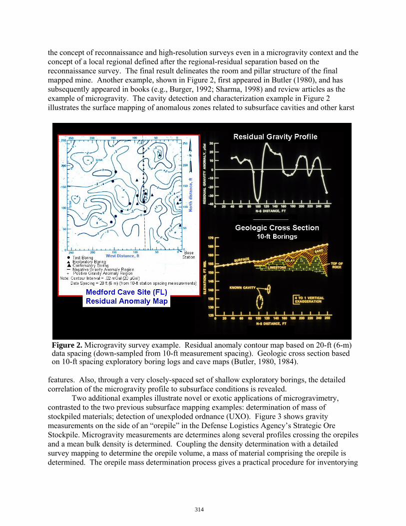
the concept of reconnaissance and high-resolution surveys even in a microgravity context and the concept of a local regional defined after the regional-residual separation based on the reconnaissance survey. The final result delineates the room and pillar structure of the final mapped mine. Another example, shown in Figure 2, first appeared in Butler (1980), and has subsequently appeared in books (e.g., Burger, 1992; Sharma, 1998) and review articles as the example of microgravity. The cavity detection and characterization example in Figure 2 illustrates the surface mapping of anomalous zones related to subsurface cavities and other karst Figure 2. Microgravity survey example. Residual anomaly contour map based on 20-ft (6-m) data spacing (down-sampled from 10-ft measurement spacing). Geologic cross section based on 10-ft spacing exploratory boring logs and cave maps (Butler, 1980, 1984). features. Also, through a very closely-spaced set of shallow exploratory borings, the detailed correlation of the microgravity profile to subsurface conditions is revealed. Two additional examples illustrate novel or exotic applications of microgravimetry, contrasted to the two previous subsurface mapping examples: determination of mass of stockpiled materials; detection of unexploded ordnance (UXO). Figure 3 shows gravity measurements on the side of an “orepile” in the Defense Logistics Agency’s Strategic Ore Stockpile. Microgravity measurements are determines along several profiles crossing the orepiles and a mean bulk density is determined. Coupling the density determination with a detailed survey mapping to determine the orepile volume, a mass of material comprising the orepile is determined. The orepile mass determination process gives a practical procedure for inventorying

314

the hundred’s of piles comprising the Strategic Stockpile (Butler et al., 1997). Microgravimetry as a general tool for detection of UXO is not a viable approach, but was investigated to determine if it might fill a niche role in special circumstances, e.g., large ordnance items. As it turns out, microgravity surveying cannot even fill a niche role for this particular application. However, the survey results in Figure 4 illustrate successful detection of a nominal 5-μGal anomaly caused by a shallow UXO using 0.25 – 0.5 m gravity measure- Figure 3. Gravity measurements on the side of an orepile. ment spacing, and thus indicates some of the high-resolution capability and potential of microgravity. The gravity anomaly even indicates an elongated source with less mass on one end, corresponding to the fuse (pointed) end of the UXO. The general failure of microgravity for this application represents a failure of intuition and lack of advance investigations; contrary to intuition, the bulk density of large UXO, e.g., 2000-lb bombs, approaches that of soil and hence does not produce a gravity anomaly, which simple calculations would have indicated in advance.

µGal µGal

Contour Interval – 1 µGal

N

Distance, mDistance, m

Dis

tanc

e, m

Dis

tanc

e, m

µGal µGal

Contour Interval – 1 µGal

N

Distance, mDistance, m

Dis

tanc

e, m

Dis

tanc

e, m

Prolate Spheroid Model

Figure 4. Calculated (left) and measured (right) gravity anomalies over a 155-mm projectile, oriented approximately horizontal with nose pointing north. Depth = 9 cm to top of projectile; length = 0.637 m; diameter = 0.155 m; mass = 45.25 kg mass; and measurement spacing = 0.25 and 0.5 m (Butler, 2001).

315

High-Resolution Magnetometry Enabling Technologies and Developments Unfortunately there isn’t a common, convenient term for near-surface engineering and environmental applications of magnetometry. My first experience with a magnetometry for near-surface applications was with a fluxgate magnetometer (ca 1970’s; Figure 5), used for stationary measurements on nominal 3-6 m grids for detection of clay-filled cavities and grikes. As a vertical component, analog magnetometer, the measurements required instrument leveling, sensitivity was likely 3-5 nT, and conservatively, anomalies ≥ 10 nT were the target. An exciting advancement came with the availability of digital, proton-precession total field magnetometers. The magnetometer shown in Figure 6 (ca 1980’s) had on-board memory, programmable measurement grid definition, and dual sensors that enabled vertical gradient determination, so that the magnetic measurements were saved along with grid coordinates. (I recall that we were so proud and excited with the system shown in Figure 6 that there is no shortage of posed pictures with it!) With the proton-precession magnetometers, sensitivity was nominally 1 nT, targets < 5 nT were routinely detected in “magnetically quiet” settings, and measurements were commonly acquired on 1-2 m grids. The fluxgate and proton-precession magnetometers found considerable use in archaeological applications (Breiner, 1972) and early environmental applications (e.g., pipeline detection, buried drums, underground storage tanks, disposal trenches; Benson et al., 1984). Figure 5. Analog fluxgate magnetometer Figure 6. Digital proton-precession magnetometer (picture ca 1977). (ca 1985-1992). The arrival of readily available, digital, optically-pumped magnetometers for near-surface application in the 1990’s was heralded by high sensitivity (~ 0.01 nT) and measurement accuracy and the capability to make measurements while moving (walking or driving), with 10-Hz measurement frequency readily available (Figure 7). The high sensitivity and accuracy and achievable measurement density result in high-fidelity magnetic maps, revealing subtle magnetic expressions of geology, soil type, and topography and detection capability for small ferrous

316

targets. Magnetic measurement grids with 15-cm spacing along lines and 0.5 – 1 m line spacing are common. Figure 7. Cesium Vapor (optically pumped) Magnetometer. (a) Total field magnetometer with integrated GPS positioning; (b) Vertical gradient configuration; (c) The Naval Research Laboratory’s (NRL) Multiple Towed Array Detection System (MTADS; ca 1996). The high gradient tolerance, small physical size and easy integration with GPS positioning have led to development of hand-held and vehicular-towed arrays of magnetometers. The towed array shown in Figure 7c has eight cesium vapor magnetometers spaced at 25 cm and mounted 25 cm above ground level; and with sample rates as high as 50 Hz, data spacing along lines is 5 – 10 cm, with RTK-GPS positioning accuracy of ~ 5 cm. The towed array magnetometer systems can survey 15 acres or more in a day and produce magnetic maps that are truly “works of art,” such as Figure 8. Only two examples are presented: one which illustrates the high-resolution detail achievable with the towed magnetometer array systems; one which illustrated the use of a “standard” magnetometer survey to solve a novel problem. Example: UXO Detection and Discrimination The requirements of UXO cleanup have been a strong and major driver of developments in hardware and processing and interpretation algorithm developments in magnetometry. At the scale of the map in Figure 8, individual anomalies due to UXO and ordnance debris surrounding a former bombing target are just visible (identifiable). Also visible in Figure 8 are prominent geologic anomalies and soils anomalies associated with topography (e.g., drainage features).

317

This magnetic survey was conducted with the NRL MTADS magnetometer system as described in the previous paragraph. Key to the successful utilization of the information content of magnetic data such as displayed in Figure 8 are developments of optimized data processing software, forward and inverse modeling for discrimination of UXO (e.g., Billings, 2004; Butler, 2001; Butler et al., 2001), and investigations into the effects of geologic backgrounds on capabilities for target detection and discrimination (e.g., Leli`ever and Oldenburg, 2000; Butler, 2003). Figure 8. Total field magnetic map, acquired with NRL MTADS, of a bombing target at the Former Buckley Field, Arapahoe County, Colorado (McDonald and Nelson, 1999). Example: Novel Problem Solution The solution to a long standing problem (since the early 1950’s) at Little Rock Air Force Base was achieved by a magnetic survey and detective work (Butler and Kean, 1993). Magnetic field fluctuations were suspected to be caused by the flight approach radar or other EM source on the base that somehow interfered with magnetic compasses by coupling directly into aircraft or through the compass calibration hardstand (a concrete pad with access from the airfield taxiway-apron area). The problem was actually much simpler and more profound. The compass calibration hardstand (and indeed all concrete used on the base, including runways) was

318

constructed of concrete with magnetic aggregate (magnetite). However, the presence of the magnetic aggregate as the culprit was only revealed after noting that the entire hardstand was a very large and spatially erratic magnetic anomaly (Figure 9). Only after identifying the hardstand itself as the problem (Figure 9b,c), by eliminating possible EM sources and verifying spatial and temporal repeatability (Figure 9c), did “detective work” lead to identifying the concrete aggregate as the source of the anomalous magnetic variability (Figure 9d). Figure 9. Solution to magnetic compass calibration problems at Little Rock Air Force Base: (a) plan map of compass calibration hardstand and magnetic survey grid; (b) magnetic map of hardstand and surrounding area; (c) profile line II on two different days illustrating repeatability; (d) the solution—magnetic aggregate used in concrete!

Closure

Clearly this paper presents a very limited and personally biased view of gravity and magnetic developments for engineering and environmental applications over the past 20-30 years. And within the limited treatment, there is a clear bias or preferential treatment of microgravity. Instrumentation developments have enabled applications of gravity and magnetic methods to classes of problems not previously considered, and conversely new problems/applications have driven instrumentation development. The new applications have also driven the development of enhanced data processing capabilities that support high-fidelity mapping for detection and discrimination of targets. What does the future hold for the near-surface applications of gravity and magnetic methods? Unfortunately my ability to prognosticate has proven quite limited and I’ve become

319

much more humble and cautious in recent years. Twenty years ago, when presented with a challenging application or a proposed idea for innovation, I would often confidently proclaim, “You can’t do that! It’s not possible.” Now, when presented with the same or similar scenarios, I frequently respond, “I don’t know--maybe.” In hindsight, I understand that the change has occurred not due to any new insight or understanding of fundamental principles, but due to profound changes in my perception of what is possible now and probable in the future technologically. For the gravity method, the true dream of practitioners is real-time (continuous), microGal-accuracy, absolute gravimetry. Translated, I mean the measurement of absolute gravity to microGal sensitivity and accuracy “while moving.” The “while moving” could be continuous in the same sense as the current state of the art in magnetometry. However, most practitioners would very happily settle for real-time, microGal-accuracy relative gravimetry. Barring a major breakthrough in fundamental gravity measurement concept or approach (e.g., a viable, fieldable, quantum mechanical approach rather than a classical mechanics approach), achievement of this dream for gravimetry is likely several orders of magnitude more difficult than for magnetometry. Regardless of such a major breakthrough in gravity measurement concept, instrumentation advances will continue to allow slight decreases in the “time on station,” enhancements in measurement statistics to allow better signal to noise characterization, and further integration of GPS technology with the gravity measurement process and instrumentation. Magnetometry already has the capability of real-time, sub-nT measurement sensitivity and accuracy while moving, with “virtually” continuous measurements along the direction of travel (measurement rates of ≈ 1500 Hz are possible). The current generation of optically pumped magnetometers is limited to nominally 25-cm lateral separation due to physical size and interference; however, improved accuracy fluxgates are available that are much smaller and can operate in closer proximity. Further decreases in size and proximity are possible with the giant magnetoresistive (GMR) sensors, and improved sensitivity and accuracy with the GMR-type sensors will allow construction of very dense arrays of sensors. It doesn’t take a great leap to envision densely packed linear- and area-magnetometer arrays in either rigid frames or flexible “carpets” that sample the magnetic field virtually continuously over realistically large line lengths or areas (say > 1 m2), with on/off sampling states, where the field is measured (recorded), saved to a storage media, reset, and the cycle repeated. References ASTM, 1999, “Standard guide for using the gravity method for subsurface investigation,” D 6430-99, ASTM International, West Conshohocken, PA. Benson, Richard C., Kaufmann, Ronald D., Yuhr, Lynn, Hopkins, Richard, 2003, “Locating and characterizing abandoned mines using microgravity,” Geophysical Technologies for Detecting Underground Coal Mine Voids Forum, Office of Surface Mines, Lexington, Kentucky. Benson, Richard C., Glaccum, Robert A., and Noel, Michael R., 1984, “Geophysical techniques for sensing buried wastes and waste migration,” EPA-600/7-84-064, US Environmental Protection Agency, Las Vegas NV. Billings, S. D., 2004, “Discrimination and classification of buried unexploded ordnance using magnetometry,” IEEE Transactions of Geoscience and Remote Sensing, 42, 1241-1251.

320

Blakeley, Richard J., 1995, Potential Theory in Gravity and Magnetic Applications, Cambridge University Press. Breiner, Sheldon, and Coe, Michael D., 1972, "Magnetic exploration of the Olmec Civilization," American Scientist, Sept-Oct, 566-575. Burger, H. Robert, 1992, Exploration Geophysics of the Shallow Subsurface, Prentice-Hall. Butler, Dwain K., 1980, “Microgravimetry for geotechnical applications,” Miscellaneous Paper GL-80-6, U.S. Army Engineer Waterways Experiment Station. Butler, Dwain K., 1980, “Assessment of microgravimetric surveys for detection of elevation changes due to reservoir impoundment,” Journal of the Geotechnical Engineering Division, American Society of Civil Engineers, 107, 355-361. Butler, Dwain K., 1984, “Microgravimetric and gravity gradient techniques for detection of subsurface cavities,” Geophysics, 49, 1084-1096. Butler, Dwain K., 1985, “Topographic effects considerations in microgravity surveying,” Proceedings of the International Conference on Potential Fields in Rugged Topography, Bulletin No. 7 of the I.G.L., University of Lausanne, Switzerland, pp 34-40. Butler, Dwain K., 1991, “Tutorial: Engineering and environmental applications of microgravimetry and magnetometry,” Proceedings of the SAGEEP ’91, Knoxville, TN. Butler, Dwain K., Sjostrom, Keith J., and Llopis, Jose L., 1997, “Selected short stories on novel applications of near-surface geophysics,” The Leading Edge, 16, 1593-1600. Butler, Dwain K., 2001, “Potential fields methods for location of Unexploded ordnance,” The Leading Edge, 20, 890-895. Butler, Dwain K., 2003, “Implications of magnetic backgrounds for unexploded ordnance detection,” Journal of Applied Geophysics, 54, 111-125. Butler, Dwain K., and Llopis, Jose L., 1991, “Repeat Gravity Surveys for Anomaly Detection in an Urban Environment,” Expanded Abstracts, Sixty First Annual International Meeting, Society of Exploration Geophysicists, Houston, 534-537. Butler, Dwain K., and Kean, Thomas B. II, 1993, “Investigations of magnetic field disturbances at an air force base compass calibration hardstand,” Geophysics, 58, 434-440. Butler, Dwain K., Wolfe, Paul J., and Hansen, Richard O., 2001, “Analytical modeling of gravity and magnetic signatures of unexploded ordnance,” Journal of Environmental and Engineering Geophysics, 6, 33-46. Hare, J. L., J. F. Ferguson, C. L. V. Aiken, and J. L. Brady, 1999, “The 4-D microgravity method for waterflood surveillance: A model study for the Prudhoe Bay reservoir, Alaska,” Geophysics, 64 , 78-87.Hinze, William J., 1990, “The role of Gravity and Magnetic Methods in Engineering and Environmental Studies,” Geotechnical and EnvironmentalGeophysics, Vol I: Review and Tutorial, S. H., Ward, ed., Society of Exploration Geophysicists, Tulsa, OK. MacMillan, William Duncan., 1958, The Theory of the Potential, Dover Publications, Inc. Lakshmanan, J., and J. Montlucon, 1987, Microgravity probes the Great Pyramid : The Leading Edge, 6 , no.1, 10-17. Leli`ever Peter G., and Oldenburg, Douglas W., 2000, “Magnetic forward modeling and inversion for high susceptibility,” Geophysics Journal International, 142, 000–000 Mickus, Kevin, 2003, “The gravity method in engineering and environmental geophysics,” Proceedings of Geophysics 2003, Federal Highway Administration and Florida Department of Transportation. Neumann, R., 1967, “La gravimetrie de haute precision application aux recherches de cavites,” Geophysical Prospecting, 15, 116-134.

321

Neumann, R., 1977, “Microgravity method applied to the detection of cavities,” Proceedings of the Symposium on Detection of Subsurface Cavities, D. K. Butler, Editor, US Army Engineer Waterways Experiment Station, Vicksburg, MS. Sharma, Prem V., 1998, Environmental and Engineering Geophysics, Cambridge University Press. Telford, W. M., Geldart, L. P., Sheriff, R. E. (1990). Applied Geophysics, Cambridge University Press. Yule, D. E., M. K. Sharp, and D. K. Butler, 1998, Microgravity investigations of foundation conditions: Geophysics, 63 , no.1, 95-103.

322