Engineering Analysis of the Abouhenidi Gas Station in … · Services Market, ATM, workshop, car...

International Journal of Scientific & Engineering Research, Volume 4, Issue 11, November-2013 1970 ISSN 2229-5518

IJSER © 2013 http://www.ijser.org

Engineering Analysis of the Abouhenidi Gas Station in Yanbu Albahar

Masters Project

PREPARED BY

Hamad Mohammad Abouhneidi

Submitted to

Prof. Rafael Moras, Ph.D., P.E.

Fall 2013

IJSER

http://www.ijser.org/



Table of contents

The Abouhenidi Gas Station .............................................................................................................. 1972

Description of company ................................................................................................................. 1972

Problem description ........................................................................................................................... 1973

Literature review ............................................................................................................................... 1974

Project goal ....................................................................................................................................... 1974

Methods ............................................................................................................................................ 1976

Goodness of fit .............................................................................................................................. 1976

Simulation ..................................................................................................................................... 1977

Data Analysis .................................................................................................................................... 1977

Statistical analysis of results .............................................................................................................. 1982

Final remarks .................................................................................................................................... 1983

References......................................................................................................................................... 1985

IJSER




The Abouhenidi Gas Station

Description of company

The Abouhenidi Gas Station was founded by my father, Mohammad Abouhenidi, in December 1999, in

Yanbu Albahar, a small city in the west of Saudi Arabia (Figure 1). Only one type of gasoline was sold in

Saudi Arabia at time, when the Ministry of Municipal and Rural Affairs had many rules for gas station

owners and entrepreneurs. For instance, a certain distance between any two gas stations had to be

observed in order not to create an excessive concentration of gas stations within one single area. This aim

has now been translated into a policy according to which gas stations have to be located at a minimum of

500 meters distance from each other within a city, and 5 km if on a highway.

Figure 1. Location of Yanbu. Source: maps.google.com/ retrieved on May 5, 2013.

Today, in Saudi Arabia there are three different types of gas stations within city limits: Types A, B and C.

Only two types of gas stations may be located on the highway: Types A and B. The specifications for

each type of Gas Station are provided in Table 1. There are major differences in the types of gas stations

IJSER




that may be built in the city and on highways regarding minimum area, types of fuel, parking capacity,

and services provided. A detailed description of the features and characteristics of the gas station types is

included in the Table 2.

Problem description

The Abouhenidi gas station is a type C: gas station, as is located within city limits. According to

regulations, it can only feature tanks with capacity up to 60,000 liters. The station has two 30,000-liter

tanks. At the time the station was founded, there was no significant transportation problem since only one

type of gasoline was sold on a standardized basis, and 15 trucks was recorded as the average number of

orders per month. Nowadays the stores carries two types of gasoline (red and green).Additionally, general

increases in demand have resulted in a surge in orders from 15 to 35 trucks per week, this and other

Type A B C Minimum area required inside

the city 3000 m2 2000 m2 1200 m2

Type of pump Gasoline/ Diesel Gasoline /Diesel Only Gasoline Services Market, ATM,

workshop, car wash oil and filter change Store.

Market, ATM, car wash

Oil and filter change store.

Market, ATM, small oil change.

Minimum number of parking slots

12 8 4

Table 1. Types of gas station on the highway

Type A B

Minimum area required on the highway

8000 m2 4000 m2

Type of pump Gasoline/ Diesel Gasoline/ Diesel Services Supermarket, ATM, workshop, car wash

oil and filter change store. Super Market, ATM, workshop, Car

wash oil and filter change store.

Minimum number of parking slots 20 15

Table 2. Types of gas station on the highway

Type of Gas Stations within the city and highway

IJSER




details are provided in Table 3, in which we depict historical demand data over the last 36 months of

operation. The data were provided by store management and include monthly sale totals (in Saudi riyals,

the cost of gasoline purchases, profits, shipping cost to the gas station, the number of shipments made to

the station, and gas station Labor). The noticeable increases in the demand for gas have created a host of

delivery problems for our business. There is an explicit increase in demand for gasoline by private

consumers and by corporations, especially the businesses that use trucks on a daily basis (e.g., food and

beverage industry, retailers, transportation companies) that has to be met by increasing and enhancing the

existing offering through an analysis of the preferred gas suppliers. By the term “preferred”, I refer to

suppliers that offer a competitive price for our company, and that have acquired relevant experience in

this business.

Literature review

Douglas (1994), David (2009), and Butenko (2007), utilized a blend of simulation and optimization to

support the decision-making processes for asset management. In addition, in modern particle experiments,

one often performs an unbinned likelihood to the data. The experimenter then needs to estimate how

accurately to the function approximates the observed distribution. A number of methods have been used

to solve this problem in the past have been reported by Stephens, (1989), Aslan (2002), Zech (2002)

Narsky (2003) and Schoemaker (1995). Both of them were used very common method, which is

goodness-of-fit method.

Project goal

Our gas station had to compete with other stations. In order to enhance the economic position of the

company, we analyzed three options for the delivery of fuel to the station:

IJSER




1- Buying a new truck at the cost of SR1 400,000

2- Buying a used truck which would cost SR 150,000

3- Leasing a truck, for a cost of SR 70,000 /year

In order to determine the preferred delivery method for our business, I carried out a comprehensive

analysis to estimate a proper solution for the transportation problem. I purport to implement the following

methods: 1 At the time of this proposal, the prevalent exchange rate was 1 USD = 3.75 Saudi Riyal

Month Revenue (SR)

Gasoline cost (SR)

Gross Profit (SR)

Total shipping cost

(SR) Number of Shipments

Labor (SR)

1 302,664 251,508 51,156 7,700 35 5,200 2 287,873 236,316 51,557 7,260 33 5,200 3 313,856 263,351 50,505 7,920 36 5,200 4 318,101 260,928 57,173 7,920 36 5,200 5 311,413 260,514 50,899 7,920 36 5,200 6 293,465 240,160 53,305 7,260 33 5,200 7 301,554 256,899 44,655 7,700 35 5,200 8 299,985 245,449 54,536 7,260 33 5,200 9 314,776 269,800 44,976 7,920 36 5,200 10 319,888 262,458 57,430 7,920 36 5,200 11 308,890 258,949 49,941 7,700 35 5,200 12 299,098 249,840 49,258 7,260 33 10,400 13 312,330 264,980 47,350 7,920 36 5,200 14 330,988 274,909 56,079 8,140 37 5,200 15 290,090 247,689 42,401 7,480 34 5,200 16 319,900 264,598 55,302 7,920 36 5,200 17 312,780 265,839 46,941 7,920 36 5,200 18 313,390 267,830 45,560 7,920 36 5,200 19 338,800 274,875 63,925 8,140 37 5,200 20 327,809 264,345 63,464 7,920 36 5,200 21 316,587 268,475 48,112 7,920 36 5,200 22 319,098 269,483 49,615 7,920 36 5,200 23 314,900 261,532 53,368 7,920 36 10,400 24 294,008 249,870 44,138 7,480 34 5,200 25 297,408 245,098 52,310 7,260 33 5,200 26 298,790 245,939 52,851 7,260 33 5,200 27 335,980 268,479 67,501 7,920 36 5,200 28 337,809 270,986 66,823 8,140 37 5,200 29 339,800 278,989 60,811 8,140 37 5,200 30 327,709 263,468 64,241 7,920 36 5,200 31 335,600 277,894 57,706 8,140 37 5,200 32 296,600 245,768 50,832 7,480 34 5,200 33 303,089 255,639 47,450 7,480 34 5,200 34 308,720 255,586 53,134 7,700 35 5,200 35 314,590 267,890 46,700 7,920 36 5,200 36 296,798 248,870 47,928 7,260 33 10,400

Total 11,255,136 9,355,203 1,899,933 278,960 1,268 202,800 Table 3. Historical demand data

IJSER




1. Goodness-of-fit analysis, to determine which probability distributions would be used to model

demand data

2. Simulation, to conduct what-if analysis of the options proposed.

In our analysis we considered a sample of recent cost levels for our business and for similar businesses in

the region. We implemented into account the recent trends emerged in this field of interest, so that for

instance, if a positive trend has been evidenced in the past, it will be more likely that also the simulation

will follow this trend as well.

Methods

Goodness of fit

The goodness-of-fit hypothesis-testing procedure is designed for problems in which the population or

probability distribution is unknown. We conducted goodness-of-fit analysis on monthly sales and number

of shipments. For calculation ease a software package called StatFit® was utilized. StatFit® is provided

as a companion to the ProModel simulation package. Analysis included the Chi-Squared, Anderson-

Darling, and Kolmogorov-Smirnov tests. The hypothesis that demand data could be modeled using a

normal distribution was not rejected by any of the test and received the highest possible rank on StatFit®.

Similar results were obtained for the number of shipments. In Table 4 we show the StatFit® output for

analysis conducted on 36 months of monthly data. The fact that the P-values for the tests ranged from

0.625 to 0.775, gave us confidence that the use of the normal distribution to model sales and shipments

was indeed a good decision. Thus, we decided that a normal distribution would indeed be an appropriate

way to simulate the sales and the number of shipments per month. The simulation was carried on Excel

and is described in the following section.

Description Result data points 36 estimates maximum likelihood estimates accuracy of fit 3.e-004 level of significance 5.e-002

Normal Table 4. Goodness-of-fit results for Monthly Sales

IJSER




Simulation

The simulation model was based on the assumption that the application of financial modeling can benefit

strategic decisions on whether our business should invest on a lease truck or choose different alternatives.

Data Analysis

Due to the very high level of competition, it was important for us to investigate which option would

benefit the business. A description of the simulation analysis is provided in this section.

Option A: Leasing a truck for a cost of SR 70,000 /year

mean 312643 sigma 14516.4

Chi Squared total classes 5 interval type Equal probable net bins 5 chi**2 2.61 degrees of freedom 4 alpha 5.e-002 chi**2(4,5.e-002) 9.49 p-value 0.625 result DO NOT REJECT

Kolmogorov-Smirnov data points 36 ks stat 0.106 alpha 5.e-002 ks stat(36,5.e-002) 0.221 p-value 0.775 result Do NOT REJECT

Anderson-Darling data points 36 ad stat 0.514 alpha 5.e-002 ad stat(36,5.e-002) 2.49 p-value 0.732 result Do NOT REJECT

Auto Fit of Distributions distribution Rank Acceptance Normal(3.13e+005, 1.45e+004 100 Do NOT REJECT Lognormal(2.8e+005, 10.3, 0.505 47.9 Do NOT REJECT Uniform(2.88e+005, 3.4e+005 26.1 Do NOT REJECT Exponential(2.88e+005, 2.48e+004) 0.397 Do NOT REJECT

Table 4. Goodness-of-fit results for Monthly Sales cont. IJSER




In Table 6 we show a 60-month simulation for the leasing system, wean analysis of simulation results

reveals that expenses amounted to approximately 31.4 % of the net profit which was SR 2,365,085.

Expenses include shipping cost and labor. For option A, we simulated three factors: sales, gas cost, and

the number of fuel delivery trips. We kept labor cost fixed at SR 5200/month. For simulation analysis,

firstly we calculated the total shipping cost by using equation

Shipping cost = (number of trips) (shipment cost, which was SR 220 / trip)

Then, we calculated the total average of sales, gas cost and number of trips based on historical data shown

in Table 3. We used the standard deviation function in Excel (STDEV) to calculate the standard deviation

for sales, gas cost and number of trips. We used the mean and standard deviation values of these variables

in the simulation. The goodness-of-fit analysis suggested that we could use the normal distribution to

model the aforementioned variables. The information was used on the function

NORMINV(RAND(),Mean, STDEV) to simulate the data for the next 60 months. All prices used in the

analysis were based on market trends at the time of this report.

Months Revenue (SR) Gasoline Cost (SR)

Gross profit (SR)

Total shipping cost (SR)

Number of Shipments

Labor (SR)

1 298,019 253,669 44,349 7,700 35 5,200 2 295,135 251,081 44,054 7,920 36 5,200 3 332,659 255,499 77,160 8,580 39 5,200 4 318,809 252,683 66,126 7,480 34 5,200 5 350,733 265,832 84,901 7,260 33 5,200 6 298,298 256,061 42,237 8,140 37 5,200 7 301,995 247,113 54,882 7,700 35 5,200 8 303,907 266,397 37,510 7,700 35 5,200 9 308,789 268,602 40,187 8,140 37 5,200 10 303,828 272,984 30,844 7,920 36 5,200 11 299,391 259,679 39,712 7,260 33 5,200 12 316,631 247,846 68,785 7,480 34 5,200 13 332,700 261,034 71,666 7,260 33 5,200 14 283,936 269,854 14,083 7,700 35 5,200 15 294,376 272,275 22,101 7,700 35 5,200 16 297,887 262,801 35,086 7,700 35 5,200 17 307,361 257,204 50,157 7,260 33 5,200 18 301,733 250,189 51,544 7,920 36 5,200 19 302,218 250,761 51,457 7,480 34 5,200 20 347,009 243,717 103,292 7,700 35 5,200 21 312,833 249,282 63,551 7,480 34 5,200 22 307,701 246,464 61,236 8,140 37 5,200

Table 6. Leasing a used truck.

IJSER




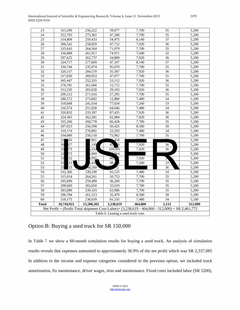
23 315,299 256,222 59,077 7,700 35 5,200 24 322,705 275,365 47,340 7,700 35 5,200 25 314,408 259,433 54,975 8,140 37 5,200 26 306,541 258,829 47,712 7,920 36 5,200 27 335,643 264,564 71,079 7,700 35 5,200 28 336,888 261,917 74,971 7,040 32 5,200 29 297,625 262,737 34,889 7,920 36 5,200 30 324,717 277,609 47,107 8,140 37 5,200 31 330,744 235,074 95,670 7,700 35 5,200 32 320,157 284,570 35,587 7,920 36 5,200 33 317,030 269,953 47,077 7,700 35 5,200 34 305,447 252,335 53,112 7,920 36 5,200 35 276,781 261,066 15,715 7,700 35 5,200 36 312,220 283,028 29,193 7,920 36 5,200 37 299,212 271,916 27,295 7,700 35 5,200 38 286,572 273,692 12,880 7,480 34 5,200 39 318,668 241,034 77,634 7,260 33 5,200 40 316,574 251,928 64,646 7,480 34 5,200 41 320,832 233,397 87,435 7,920 36 5,200 42 324,365 262,281 62,084 7,920 36 5,200 43 335,206 268,778 66,428 7,700 35 5,200 44 307,023 256,598 50,425 8,580 39 5,200 45 310,174 276,881 33,293 7,480 34 5,200 46 334,080 258,118 75,962 7,700 35 5,200 47 312,420 250,961 61,458 7,700 35 5,200 48 306,827 261,149 45,678 7,920 36 5,200 49 355,475 245,534 109,941 7,920 36 5,200 50 323,473 266,909 56,564 8,140 37 5,200 51 331,232 244,995 86,237 7,920 36 5,200 52 313,613 264,438 49,175 7,260 33 5,200 53 257,233 248,260 8,972 7,920 36 5,200 54 332,366 239,240 93,125 7,480 34 5,200 55 315,014 264,261 50,753 7,700 35 5,200 56 295,699 259,499 36,200 7,700 35 5,200 57 298,669 265,650 33,019 7,700 35 5,200 58 303,089 239,103 63,986 7,700 35 5,200 59 296,784 261,313 35,470 8,580 39 5,200 60 318,175 236,639 81,535 7,480 34 5,200

Total 18,744,921 15,506,302 3,238,619 464,860 2,113 312,000 Net Profit = (Profit-Total shipment Cost-Labor)= (3,238,619 - 464,860 - 312,000) = SR 2,461,772

Table 6. Leasing a used truck cont.

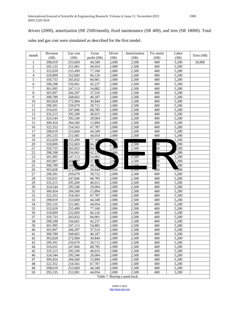
Option B: Buying a used truck for SR 150,000

In Table 7 we show a 60-month simulation results for buying a used truck. An analysis of simulation

results reveals that expenses amounted to approximately 36.9% of the net profit which was SR 2,337,085

In addition to the income and expense categories considered in the previous option, we included truck

amortization, fix maintenance, driver wages, tires and maintenance. Fixed costs included labor (SR 5200),

IJSER




drivers (2000), amortization (SR 2500/month), fixed maintenance (SR 400), and tires (SR 18000). Total

sales and gas cost were simulated as described for the first model.

month Revenue (SR)

Gas cost (SR)

Gross profit (SR)

Driver (SR)

Amortization (SR)

Fix maint (SR)

Labor (SR) Tires (SR)

1 298,019 253,669 44,349 2,000 2,500 400 5,200 18,000 2 295,135 251,081 44,054 2,000 2,500 400 5,200

3 332,659 255,499 77,160 2,000 2,500 400 5,200 4 318,809 252,683 66,126 2,000 2,500 400 5,200 5 350,733 265,832 84,901 2,000 2,500 400 5,200 6 298,298 256,061 42,237 2,000 2,500 400 5,200 7 301,995 247,113 54,882 2,000 2,500 400 5,200 8 303,907 266,397 37,510 2,000 2,500 400 5,200 9 308,789 268,602 40,187 2,000 2,500 400 5,200 10 303,828 272,984 30,844 2,000 2,500 400 5,200 11 299,391 259,679 39,712 2,000 2,500 400 5,200 12 316,631 247,846 68,785 2,000 2,500 400 5,200 13 335,215 295,200 40,015 2,000 2,500 400 5,200 14 324,544 295,540 29,004 2,000 2,500 400 5,200 15 300,454 284,560 15,894 2,000 2,500 400 5,200 16 322,352 254,565 67,787 2,000 2,500 400 5,200 17 298,019 253,669 44,349 2,000 2,500 400 5,200 18 295,135 251,081 44,054 2,000 2,500 400 5,200 19 332,659 255,499 77,160 2,000 2,500 400 5,200 20 318,809 252,683 66,126 2,000 2,500 400 5,200 21 350,733 265,832 84,901 2,000 2,500 400 5,200 22 298,298 256,061 42,237 2,000 2,500 400 5,200 23 301,995 247,113 54,882 2,000 2,500 400 5,200 24 303,907 266,397 37,510 2,000 2,500 400 5,200 25 308,789 268,602 40,187 2,000 2,500 400 5,200 26 303,828 272,984 30,844 2,000 2,500 400 5,200 27 299,391 259,679 39,712 2,000 2,500 400 5,200 28 316,631 247,846 68,785 2,000 2,500 400 5,200 29 335,215 295,200 40,015 2,000 2,500 400 5,200 30 324,544 295,540 29,004 2,000 2,500 400 5,200 31 300,454 284,560 15,894 2,000 2,500 400 5,200 32 322,352 254,565 67,787 2,000 2,500 400 5,200 33 298,019 253,669 44,349 2,000 2,500 400 5,200 34 295,135 251,081 44,054 2,000 2,500 400 5,200 35 332,659 255,499 77,160 2,000 2,500 400 5,200 36 318,809 252,683 66,126 2,000 2,500 400 5,200 37 350,733 265,832 84,901 2,000 2,500 400 5,200 38 298,298 256,061 42,237 2,000 2,500 400 5,200 39 301,995 247,113 54,882 2,000 2,500 400 5,200 40 303,907 266,397 37,510 2,000 2,500 400 5,200 41 308,789 268,602 40,187 2,000 2,500 400 5,200 42 303,828 272,984 30,844 2,000 2,500 400 5,200 43 299,391 259,679 39,712 2,000 2,500 400 5,200 44 316,631 247,846 68,785 2,000 2,500 400 5,200 45 335,215 295,200 40,015 2,000 2,500 400 5,200 46 324,544 295,540 29,004 2,000 2,500 400 5,200 47 300,454 284,560 15,894 2,000 2,500 400 5,200 48 322,352 254,565 67,787 2,000 2,500 400 5,200 49 298,019 253,669 44,349 2,000 2,500 400 5,200 50 295,135 251,081 44,054 2,000 2,500 400 5,200 Table 7. Buying a used truck.

IJSER




51 332,659 255,499 77,160 2,000 2,500 400 5,200 52 318,809 252,683 66,126 2,000 2,500 400 5,200 53 350,733 265,832 84,901 2,000 2,500 400 5,200 54 298,298 256,061 42,237 2,000 2,500 400 5,200 55 301,995 247,113 54,882 2,000 2,500 400 5,200 56 303,907 266,397 37,510 2,000 2,500 400 5,200 57 308,789 268,602 40,187 2,000 2,500 400 5,200 58 303,828 272,984 30,844 2,000 2,500 400 5,200 59 299,391 259,679 39,712 2,000 2,500 400 5,200 60 316,631 247,846 68,785 2,000 2,500 400 5,200 Total 18,760,460 15,779,375 2,981,085 120,000 150,000 24,000 312,000 18,000

Net Profit

= (Profit- Labor –Amortization- Fix maintenance - Driver wage -Tires) = (2,981,085 - 120,000 - 150,000 - 24,000 - 312,000) = SR 2,337,085

Table 7. Buying a used truck cont.

Option C: Buying a new truck for SR 400,000

In Table 8 we show a 60-month of simulation of the decision to acquire a new truck. An analysis of

simulation results reveals that expenses amounted to approximately 40.98% from the total profit, which is

SR 2,305,633 and includes the amortization, driver and Labor. However, if we bought a new truck, we

would receive free maintenance. In this model, the fixed factors were labor (SR 5,200) the truck drivers

(SR 2,000), and amortization (SR 6,667 /month). The simulation analysis was similar to that conducted

before.

Month Revenue (SR) Gas cost(SR) Gross profit (SR) Driver (SR) Amortization

(SR) Labor (SR)

1 298,019 253,669 44,349 2,000 6,667 5,200 2 295,135 251,081 44,054 2,000 6,667 5,200 3 332,659 255,499 77,160 2,000 6,667 5,200 4 318,809 252,683 66,126 2,000 6,667 5,200 5 350,733 265,832 84,901 2,000 6,667 5,200 6 298,298 256,061 42,237 2,000 6,667 5,200 7 301,995 247,113 54,882 2,000 6,667 5,200 8 303,907 266,397 37,510 2,000 6,667 5,200 9 308,789 268,602 40,187 2,000 6,667 5,200 10 303,828 272,984 30,844 2,000 6,667 5,200 11 299,391 259,679 39,712 2,000 6,667 5,200 12 316,631 247,846 68,785 2,000 6,667 5,200 13 305,455 254,498 50,957 2,000 6,667 5,200 14 298,500 250,985 47,515 2,000 6,667 5,200 15 301,511 254,674 46,837 2,000 6,667 5,200 16 312,500 254,647 57,853 2,000 6,667 5,200 17 298,019 253,669 44,349 2,000 6,667 5,200 18 295,135 251,081 44,054 2,000 6,667 5,200 19 332,659 255,499 77,160 2,000 6,667 5,200 20 318,809 252,683 66,126 2,000 6,667 5,200

Table 8. Simulation data for the option of acquiring a new truck.

IJSER




21 350,733 265,832 84,901 2,000 6,667 5,200 22 298,298 256,061 42,237 2,000 6,667 5,200 23 301,995 247,113 54,882 2,000 6,667 5,200 24 303,907 266,397 37,510 2,000 6,667 5,200 25 308,789 268,602 40,187 2,000 6,667 5,200 26 303,828 272,984 30,844 2,000 6,667 5,200 27 299,391 259,679 39,712 2,000 6,667 5,200 28 316,631 247,846 68,785 2,000 6,667 5,200 29 305,455 254,645 50,810 2,000 6,667 5,200 30 298,500 250,454 48,046 2,000 6,667 5,200 31 305,444 256,410 49,034 2,000 6,667 5,200 32 312,500 254,647 57,853 2,000 6,667 5,200 33 298,019 253,669 44,349 2,000 6,667 5,200 34 295,135 251,081 44,054 2,000 6,667 5,200 35 332,659 255,499 77,160 2,000 6,667 5,200 36 318,809 252,683 66,126 2,000 6,667 5,200 37 350,733 265,832 84,901 2,000 6,667 5,200 38 298,298 256,061 42,237 2,000 6,667 5,200 39 301,995 247,113 54,882 2,000 6,667 5,200 40 303,907 266,397 37,510 2,000 6,667 5,200 41 308,789 268,602 40,187 2,000 6,667 5,200 42 303,828 272,984 30,844 2,000 6,667 5,200 43 299,391 259,679 39,712 2,000 6,667 5,200 44 316,631 247,846 68,785 2,000 6,667 5,200 45 305,455 254,645 50,810 2,000 6,667 5,200 46 298,500 250,454 48,046 2,000 6,667 5,200 47 305,444 256,410 49,034 2,000 6,667 5,200 48 312,500 254,647 57,853 2,000 6,667 5,200 49 298,019 253,669 44,349 2,000 6,667 5,200 50 295,135 251,081 44,054 2,000 6,667 5,200 51 332,659 255,499 77,160 2,000 6,667 5,200 52 318,809 252,683 66,126 2,000 6,667 5,200 53 350,733 265,832 84,901 2,000 6,667 5,200 54 298,298 256,061 42,237 2,000 6,667 5,200 55 301,995 247,113 54,882 2,000 6,667 5,200 56 303,907 266,397 37,510 2,000 6,667 5,200 57 308,789 268,602 40,187 2,000 6,667 5,200 58 303,828 272,984 30,844 2,000 6,667 5,200 59 299,391 259,679 39,712 2,000 6,667 5,200 60 316,631 247,846 68,785 2,000 6,667 5,200

Total 18,574,529 15,436,896 3,137,633 120,000 400,000 312,000

Net Profit = (Profit- Labor - Amortization - Driver wages - Tires) = (3,137,633 - 120,000 - 312,000) = SR 2,305,633

Table 8. Simulation data for the option of acquiring a new truck cont.

Statistical analysis of results

An analysis of simulation results revealed that the differences in the bottom line figures among

the alternatives was relatively small. We proceeded to conduct ANOVA analysis of the

simulation results. The null hypothesis was that the mean value of the net profits resulting from

IJSER




the three decisions (buy new car, buy used car, lease) were equal. The alternate hypothesis was

that at least one of the mean values would be different. Sixty replications for each decision were

used. The response variable was Net Profits, which was given by the formula

Net profits = Revenue – ∑𝐴𝑙𝑙 𝑐𝑜𝑠𝑡𝑠

A simple ANOVA model was used with a single factor (decision) with three levels (buying a

new truck, buying a used truck, or leasing). A software package called Design Expert ® was

utilized. As shown in Table 9, the differences in the response variable were not statistically

significant at the 5 percent significance level, and that the null hypothesis that the mean net profit

figures were equal could not be rejected.

Analysis of variance table [Classical sum of squares - Type II] Sum of Mean F Source Squares df Square Value p value Model 2.174E+008 2 1.087E+008 0.30 0.7413 Pure Error 6.415E+010 177 3.624E+008 Cor Total 6.437E+010 179

Table 9. Analysis of variance of simulation results.

Final remarks

Statistical analysis of the decision making process of the Abouhenidi Gas Station of Yanbu, Saudi Arabia,

was conducted. The analysis included the following components:

1. Data collection. Demand data over a 36-month study period was provided by Management.

2. Goodness-of-fit tests. The use of the package StatFit® suggested that the normal distribution

could be used to model monthly revenues, fuel cost, and the number of delivery trips made by

supplier trucks to the station.

IJSER




3. Simulation. We used Excel to simulate fuel sales over a 60-month study period under three

scenarios: (1) buying a new delivery truck, (2) buying a used delivery truck, (3) leasing a delivery

truck.

4. Analysis of variance. The simulation results were fed to an ANOVA package called Design

Expert®. The hypothesis that the net profits yielded by the three alternatives were equal could

not be rejected.

The station owner was informed about the results of this study. His opinion is that since the null

hypothesis could not be rejected, he would opt to implement the decision that would minimize the

perceived risk. He favored the lease alternative, as it minimized the risks presented by maintenance. The

author plans to enhance the simulation model in the future to continue to aid in the decision making

process at the gas station. A possible embellishment is the implementation of a conditional rule in the

Used Truck alternative by which the ownership would decide to sell the used truck if the cumulative

maintenance cost reached a certain threshold. The station would switch to leasing a truck from that point

on.

IJSER




References

Wikipedia, (2013).Yanbu

http://tl.wikipedia.org/wiki/Yanbu (consulted on May 16, 2013)

The Ministry of Municipal and Rural Affairs (2013). A list of gas stations, with washing and lubricating facilities.

http://www.momra.gov.sa/generalserv/specs/spec0001-3.asp?print=true (consulted on June 21, 2013).

Douglas, C, (1994). Applied statistics and probability for Engineering. Goodness of fit, 8 (11), 444-446.

David, S, (2009). Statistics concepts and controversies, Simulation, 19(5), 411-428.

Butenko, S, (2007) Asset management literature review and potential applications of simulation, optimization, and decision analysis techniques for right-of-way and transportation planning and programming.

D'Agostino, R, and Stephens, M, (1989) “Goodness- of- fit Techniques”

Aslan, B, (2002) “A new class of binning free, multivariate goodness-of-fit tests”

Narsky, I, (2003) “Goodness of Fit: What Do We Really Want to Know?”

Shoemaker, PGH, (1995) “Scenario Planning: A Tool for strategic Thinking”

IJSER


http://tl.wikipedia.org/wiki/Yanbu

http://www.momra.gov.sa/generalserv/specs/spec0001-3.asp?print=true



IJSER


Engineering Analysis of the Abouhenidi Gas Station in … · Services Market, ATM, workshop, car...

Documents

Transcript of Engineering Analysis of the Abouhenidi Gas Station in … · Services Market, ATM, workshop, car...