Engineering Analysis ENG 3420 Fall 2009

Dan C. Marinescu

Office: HEC 439 B

Office hours: Tu-Th 11:00-12:00

22Lecture 11

Lecture 11

Last time: Newton-Raphson The secant method

Today: Optimization

Golden ratio makes one-dimensional optimization efficient. Parabolic interpolation locate the optimum of a single-variable function. fminbnd function determine the minimum of a one-dimensional

function. fminsearch function determine the minimum of a multidimensional

function.

Next Time Linear algebra

Optimization Critical for solving engineering and scientific problems.

One-dimensional versus multi-dimensional optimization. Global versus local optima. A maximization problem can be solved with a minimizing algorithm.

Optimization is a hard problem when the search space for the optimal solution is very large. Heuristics such as simulated annealing, genetic algorithms, neural networks.

Algorithms Golden ratio makes one-dimensional optimization efficient. Parabolic interpolation locate the optimum of a single-variable function. fminbnd function determine the minimum of a one-dimensional function. fminsearch function determine the minimum of a multidimensional function.

How to develop contours and surface plots to visualize two-dimensional functions.

3

Optimization

Find the most effective solution to a problem subject to a certain criteria. Find the maxima and/or minima of a function of one or more variables.

One- versus multi-dimensional optimization One-dimensional problems involve functions that depend on a

single dependent variable -for example, f(x). Multidimensional problems involve functions that depend on two

or more dependent variables - for example, f(x,y)

Global versus local optimization

Global optimum the very best solution. Local optimum solution better than its immediate neighbors.

Cases that include local optima are called multimodal. Generally we wish to find the global optimum.

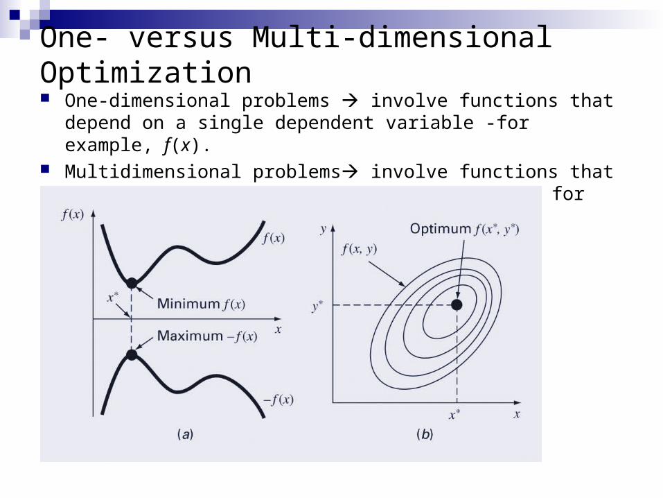
One- versus Multi-dimensional Optimization One-dimensional problems involve functions that depend on a

single dependent variable -for example, f(x). Multidimensional problems involve functions that depend on two

or more dependent variables - for example, f(x,y)

Euclid’s golden number

Given a segment of length the golden number

is determined from the condition:

The solution of the last equation is

8

21 yy 2

1

y

y

012

2

21

2

2

1

y

yy

y

y

680133.12

51

Golden-Section Search Algorithm for finding a minimum on an interval [xl xu] with a single

minimum (unimodal interval); uses the golden ratio =1.6180 to determine location of two interior points x1 and x2;

One of the interior points can be re-used in the next iteration. f(x1)<f(x2) x2 will be the new lower limit and x1 the new x2.

f(x2)<f(x1) x1 will be the new upper limit and x2 the new x1.

d ( 1)(xu x l )x1 x l dx2 xu d

f(x1)<f(x2) x2 is the new lower limit and x1 the new x2 .

f(x2)<f(x1) x1 is the new upper limit and x2 the new x1.

Golden section versus bisection

11

Parabolic interpolation

Parabolic interpolation requires three points to estimate optimum location.

The location of the maximum/minimum of a parabola defined as the interpolation of three points (x1, x2, and x3) is:

The new point x4 and the two surrounding it (either x1 and x2 or x2 and x3) are used for the

next iteration of the algorithm.

x4 x2 1

2

x2 x1 2 f x2 f x3 x2 x3 2 f x2 f x1 x2 x1 f x2 f x3 x2 x3 f x2 f x1

fminbnd built-in function

fminbnd combines the golden-section search and the parabolic interpolation.

Example [xmin, fval] = fminbnd(function, x1, x2)

Options may be passed through a fourth argument using optimset, similar to fzero.

fminsearch built-in function

fminsearch determine the minimum of a multidimensional function. [xmin, fval] = fminsearch(function, x0)

xmin a row vector containing the location of the minimum x0 an initial guess; must contain as many entries as the function

expects.

The function must be written in terms of a single variable, where different

dimensions are represented by different indices of that variable.

Example: minimize f(x,y)=2+x-y+2x2+2xy+y2

Step 1: rewrite as:

f(x1, x2)=2+x1-x2+2(x1)2+2x1x2+(x2)2

Step 2: define the function f using Matlab syntax: f=@(x) 2+x(1)-x(2)+2*x(1)^2+2*x(1)*x(2)+x(2)^2 Step 3: invoke fminsearch

[x, fval] = fminsearch(f, [-0.5, 0.5])x0 has two entries - f is expecting it to contain two values.the minimum value is 0.7500 at a location of [-1.000 1.5000]

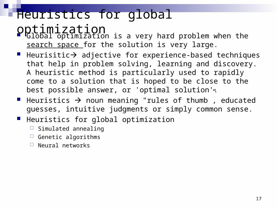
Heuristics for global optimization Global optimization is a very hard problem when the search space

for the solution is very large. Heurisitic adjective for experience-based techniques that help in

problem solving, learning and discovery. A heuristic method is particularly used to rapidly come to a solution that is hoped to be close to the best possible answer, or 'optimal solution'.

Heuristics noun meaning "rules of thumb”, educated guesses, intuitive judgments or simply common sense. 

Heuristics for global optimization Simulated annealing Genetic algorithms Neural networks

17

Simulated annealing (SA)

Inspired from metallurgy: Annealing is a technique involving heating and controlled cooling of a material to

increase the size of its crystals and reduce their defects. The heat causes the atoms to become unstuck from their initial positions (a local

minimum of the internal energy) and wander randomly through states of higher energy; the slow cooling gives them more chances of finding configurations with lower internal energy than the initial one.

Each step of the SA algorithm: Replaces the current solution by a random "nearby" solution, chosen with a

probability that depends on the difference between the corresponding function values and on a global parameter T (called the temperature), that is gradually decreased during the process.

The dependency is such that the current solution changes almost randomly when T is large, but increasingly "downhill" as T goes to zero. The allowance for "uphill" moves saves the method from becoming stuck at local minima—which are the bane of greedier methods.

18

Genetic algorithms Global search heuristics to find exact or approximate solutions

to optimization and search problems. Genetic algorithms are a particular class of evolutionary algorithms (EA) that use evolutionary biology concepts such as inheritance, mutation, selection, and crossover.

 The evolution usually starts from a population of randomly generated individuals and happens in generations. In each generation, the fitness of every individual in the population is evaluated, multiple individuals are stochastically selected from the current population (based on their fitness), and modified (recombined and possibly randomly mutated) to form a new population. The new population is then used in the next iteration of the algorithm. Commonly, the algorithm terminates when either a maximum number of generations has been produced, or a satisfactory fitness level has been reached for the population. If the algorithm has terminated due to a maximum number of generations, a satisfactory solution may or may not have been reached.

19

Neural networks Biological neural networks are made up of real biological neurons

that are connected or functionally related in the  peripheral nervous system or the central nervous system. In the field of neuroscience, they are often identified as groups of neurons that perform a specific physiological function in laboratory analysis.

Artificial neural networks  are made up of interconnecting artificial neurons (programming constructs that mimic the properties of biological neurons). Artificial neural networks may either be used to gain an understanding of biological neural networks, or for solving artificial intelligence problems without necessarily creating a model of a real biological system.

20

Nedler Mead optimization

Heuristic Consider N+1 equidistant points in space.

Evaluate the function at these points. Throw away the worse results by projecting the point through a

centroid formed by all the other remaining points Many variations exist to improve performance

More info at http://www.ces.clemson.edu/me/credo/classes/Integropt2-29.pdf

21

Contour and surface/mesh plots are used to visualize functions of two-variables

23

subplot  divides the current figure into rectangular panes numbered row-wise. Each pane contains an axes; subsequent plots are output to the current pane.

subplot(m,n,p)  creates an axes in the p-th pane of a figure divided into an m-by-n matrix of rectangular panes. The new axes becomes the current axes.

linspace  generates linearly spaced vectors. It is similar to the colon operator ":", but gives direct control over the number of points.

y = linspace(a,b)  generates a row vector y of 100 points linearly spaced between and including a and b.y = linspace(a,b,n)  generates a row vector y of n points linearly spaced between and including a and b. For n < 2, linspace returns b.

[X,Y] = meshgrid(x,y)  transforms the domain specified by vectors x and y into arrays X and Y, which can be used to evaluate functions of two variables and three-dimensional mesh/surface plots. The rows of the output array X are copies of the vector x; columns of the output array Y are copies of the vector y.

clabel(C)  adds labels to the current contour plot using the contour array C output from contour. The function labels all contours displayed and randomly selects label positions.

Plot:

x=linspace(-2,0,40);

y=linspace(0,3,40);

[X,Y]=meshgrid(x,y);

Z=2+X-Y+2*X.^2+2*X.*Y+Y.^2;

subplot(1,2,1);

cs=contour(X,Y,Z);clabel(cs);

xlabel(‘x_1’);ylabel(‘x_2’);

title(‘(a) Contour plot’):grid;

subplot(1,2,2);

cs=surfc(X,Y,Z);

zmin=floor(min(Z));

zmax=cell(max(Z));

xlabel(‘x_1’); ylabel(‘x_2’); zlabel(‘f(x_1,x_2)’);

title(‘(b) Mesh plot’);

24

2221

212121 222),( xxxxxxxxf