Engineering 12 Physical systems analysis

Laboratory 3: The Coupled Pendulums system

Swarthmore College Department of Engineering Jeff Santer ‘09, Nick Villagra ‘09, Rio Akasaka ‘09

System behavior of two coupled pendulums when one is stationary and the other is released at an angle.

Abstract

This experiment examines the behavior of a system consisting of two pendulums

coupled by a spring. The motion of the pendulums was derived mathematically, after

which the system was modeled in Matlab’s Simulink and plotted. The discrepancy

between experimental and theoretical values for the frequency were within 8% error,

highlighting remarkable similarities despite significant sources of error. The angular

frequency obtained for pendulum 1 was 4.2302 radians, and was 4.3592 for pendulum 2.

The spring used for the experiment was found to have a spring constant K value of 24.12.

Introduction To deepen understanding of oscillatory motion, analysis was conducted of a

coupled pendulum system under three different sets of initial conditions. After obtaining

experimental data from the motion of tion were

analytically derived by summi s and applying

state variables to the angular displacem

pendulums. The program Simu m

system and thereby obtain theoretical representations of the oscillatory motion. The

experimental results of motion served to verify the accuracy and thereby the utility of the

analytical methods previously described, such as deriving state variable equations and

using the program Simulink. This experiment introduces the tools and methodology

necessary for broadly analyzing the oscillatory behavior of swinging masses, an

important physical concept that is applicable to the fields of bridge design and skyscraper

design.

the pendulums, equations of mo

ng the forces acting on each of the pendulum

ents and angular velocities of the respective

link was also used to recreate the coupled pendulu

Theory

This experiment deals with a system of coupled pendulums, set up as shown in

Figure 2. A free body diagram is shown below in Figure 1.

Figure 1. Free Body Diagram of Pendulum 1

Summing the torques caused by the above forces, using the small angle approximation

that sinθ ≈ θ and cosθ ≈ 1, and setting the

equations of motion. We assume that the

concentrated at a point, which means that

pendulums are found to be:

θmgθm

θmgθm

22

22

12

12

+

++

l&&l

l&&l

Making the substitutions

sum of the forces equal to Jθ&& gives the

rod is massless and the mass at the end is

2J m= l . The equations of motion for both

0)θθ(k

0)θθ(k

122

212

=−+

=−

s

s

l

l

22 2 s1 2

g km

⎛ ⎞κ = ⎜ ⎟⎝ ⎠

l

l lallows us to easily write the andκ =

system as below.

( ) 22 1 2 2 0θ − κ θ =

( )

2 21 1

2 2 22 1 2 2 2 1 0.

θ + κ + κ

θ + κ + κ θ − κ θ =

&&

&&

The following substitutions are then made to rewrite the equations in state-variable form:

1 1

2 2

3 1 1

4 2 2

xx

x xx x

= θ= θ

= θ == θ =

& && &

In state variable form, the equations of motion are thus:

( )( )

11

222 2 21 2 2 11

2 2 222 2 1 2

0 0 1 00 0 0 1

0 0

0 0

⎡ ⎤⎡ ⎤ θθ ⎡ ⎤⎢ ⎥⎢ ⎥ ⎢ ⎥θ⎢ ⎥θ⎢ ⎥ ⎢ ⎥= •⎢ ⎥− κ + κ κ⎢ ⎥ ⎢ ⎥ωω ⎢ ⎥⎢ ⎥ ⎢ ⎥⎢ ⎥ ωω⎢ ⎥ κ − κ + κ ⎣ ⎦⎣ ⎦ ⎣ ⎦

&

&

&

&

Now, we must find the eigenvalues and eigenvectors of the matrix M that is multiplied by

the state variables. To find this, we set det (λI-M) = 0, where the eigenvalue λ is a

constant, and Ι is the identity matrix. We therefore have:

( )( )

2 21 2

2 22 1

22

22

0 1 00 0 1

00

0

λ −λ −

=κ + κ −

−κ κ +

Working this out:

( )

κ λ

κ λ

( )( )

2 2 2 22 1 2 2

2 2 22 1 2

0 1

0 0 0

λ −

κ + κ −κ − =

−κ κ + κ λ

( ) ( )

2 21 2

0 10 0 1

0

λ −λ −κ λ − + −

κ + κ λ

Simplifying:

( )( ) ( )22 2 4 2 2 21 2 2 1 2 0+ κ + κ − λ κ + κ = 3 2 2

1 2λ λ + λ κ + κ − − κ

( ) ( )2 2 4 2 2 21 2 2 1 22 0κ κ − κ + λ κ + κ = 4 2 2 2 4 4

1 2 1 2λ + λ κ + κ + κ + κ +

( )2 4 2 21 1 22 2 0+ κ + κ κ =

e equation using the quadratic formula.

4 2 21 2λ + λ κ + κ

By making the substitution q=λ2, we can solve th

( ) ( )22 2 2 2 4 2 21 2 1 2 1 1 2

2 2 41 2 2

2 2 21,2 1 1 2

2 21,2,3,4 1,2 1 1 2

q 2

q

q , 2

q j , j 2

= − κ + κ ± κ + κ − κ − κ κ

= −κ − κ ± κ

= −κ −κ − κ

∴λ = ± = ± κ ± κ + κ

Now, we must find the eigenvectors by solving the matrix equation λ j I − M[ ]•V j = 0 for

each eigenvalue/eigenvector pair, where M is the matrix from the state-variable equation.

( )( )

( ) ( )( ) ( )

11,1

11,2

2 2 21 2 2 1 1,3

2 2 21,42 1 2 1

1 1,1 1,3

1 1,2 1,4

2 2 21 2 1,1 2 1,2 1 1 1,1

2 2 22 1,1 1 2 1,2 1 1 1,2

1 1

j 0 1 0 V0 j 0 1 V

0j 0 VV0 j

The last two equj V Vj V V

V V j j V 0

V V j j V

j

κ −⎡ ⎤ ⎡ ⎤⎢ ⎥ ⎢ ⎥κ −⎢ ⎥ ⎢ ⎥ =⎢ ⎥κ + κ −κ κ ⎢ ⎥⎢ ⎥ ⎢ ⎥⎢ ⎥−κ κ + κ κ ⎣ ⎦⎣ ⎦

κ =

κ = ⇒κ + κ − κ + κ κ =

−κ + κ + κ + κ κ =

λ = κ

1,1

1,2

1,3 11,1 1,2

V 1ationsV 1show thatV jV V

⎡ ⎤ ⎡ ⎤⎢ ⎥ ⎢ ⎥⎢ ⎥ ⎢ ⎥⇒ =⎢ ⎥ ⎢ ⎥κ=⎢ ⎥ ⎢ ⎥

01,4 1V jSo κ⎣ ⎦⎣ ⎦

( )( )

( ) ( )( ) ( )

12,1

12,2

2 2 21 2 2 1 2,3

2 2 22,42 1 2 1

1 2,1 2,3

1 2,2 2,4

2 2 21 2 2,1 2 2,2 1 1 2,1

2 2 22 2,1 1 2 2,2 1 1 2,2

j 0 1 0 V0 j 0 1 V

j 0 VV0 j

j V Vj V V

V V j j V

V V j j V

− κ −⎡ ⎤ ⎡ ⎤⎢ ⎥ ⎢ ⎥− κ −⎢ ⎥ ⎢ ⎥⎢ ⎥κ + κ −κ − κ ⎢ ⎥⎢ ⎥ ⎢ ⎥⎢ ⎥−κ κ + κ − κ ⎣ ⎦⎣ ⎦

− κ =

− κ =

κ + κ − κ − κ − κ =

−κ + κ + κ − κ − κ =

2 10

The las

0

0

j=

⇒

λ = − κ

2,1

2,2

2,3 12,1 2,2

2,4 1

V 1t two equationsV 1show thatV jV VV jSo

⎡ ⎤ ⎡ ⎤⎢ ⎥ ⎢ ⎥⎢ ⎥ ⎢ ⎥⇒ =⎢ ⎥ ⎢ ⎥− κ=⎢ ⎥ ⎢ ⎥− κ⎣ ⎦⎣ ⎦

( )( )

( )

2 21 2

3,12 21 2 3,2

2 2 2 2 23,31 2 2 1 2

3,42 2 2 2 22 1 2 1 2

2 21 2 3,1 3,3

2 21 2 3,2 3,4

2 2 2 2 2 2 21 2 3,1 2 3,2 1 2 1 2

2 21 23

j 2 0 1 0 V0 j 2 0 1 V

0Vj 2 0V

0 j 2

j 2 V V

j 2 V V

V V j 2 j 2

j 2

⎡ ⎤κ + κ − ⎡ ⎤⎢ ⎥⎢ ⎥⎢ ⎥κ + κ −⎢ ⎥⎢ ⎥ =⎢ ⎥⎢ ⎥κ + κ −κ κ + κ⎢ ⎥⎢ ⎥⎣ ⎦⎢ ⎥−κ κ + κ κ + κ⎣ ⎦

κ + κ =

κ + κ =

κ + κ − κ + κ + κ κ + κ

κ + κλ =

( )( ) ( )

3,1

3,22 2

3,3 1 23,1 3,23,1 2 23,4 1 2

2 2 2 2 2 2 22 3,1 1 2 3,2 1 2 1 2 3,2

1VThe last two equations1Vshow that

V j 2V VV 0

VSo j 2V V j 2 j 2 V 0

⎡ ⎤⎡ ⎤⎢ ⎥⎢ ⎥ −⎢ ⎥⎢ ⎥⇒ ⇒ = ⎢ ⎥⎢ ⎥ κ + κ= − ⎢ ⎥= ⎢ ⎥⎢ ⎥− κ + κ⎣ ⎦ ⎣ ⎦

−κ + κ + κ + κ + κ κ + κ =

___________________________________________________________________________

( )( )

( )

2 21 2

4,12 21 2 4,2

2 2 2 2 24,31 2 2 1 2

4,42 2 2 2 22 1 2

2 21 2 4,1 4,3

2 21 2 4,2 4,4

2 2 2 2 21 2 4,1 2 4,2 1 2

2 21 23

j 2 0 1 0 V0 j 2 0 1 V

0Vj 2 0V

0 j

j 2 V V

j 2 V V

V V j 2 j

j 2

⎡ ⎤− κ + κ − ⎡ ⎤⎢ ⎥⎢ ⎥⎢ ⎥− κ + κ −⎢ ⎥⎢ ⎥ =⎢ ⎥⎢ ⎥κ + κ −κ − κ + κ⎢ ⎥⎢ ⎥⎣ ⎦⎢ ⎥−κ κ + κ −

− κ + κ =

− κ + κ =

κ + κ − κ − κ + κ −

κ + κλ = −

1 22κ + κ⎣ ⎦

(( )

)( )

4,1

4,22 2

4,3 1 24,1 4,24,1 2 24,4 1 2

22 4,2

1VThe last two equations1Vshow that

V j 2V V2 V 0

VSo j 22 V 0

2 21 2

2 2 2 2 2 22 4,1 1 2 4,2 1 2 1V V j 2 j

⎡ ⎤⎡ ⎤⎢ ⎥⎢ ⎥ −⎢ ⎥⎢ ⎥⇒ ⇒ = ⎢ ⎥⎢ ⎥ − κ + κ= − ⎢ ⎥= ⎢ ⎥κ + κ⎢ ⎥κ + κ⎣ ⎦ ⎣ ⎦

=

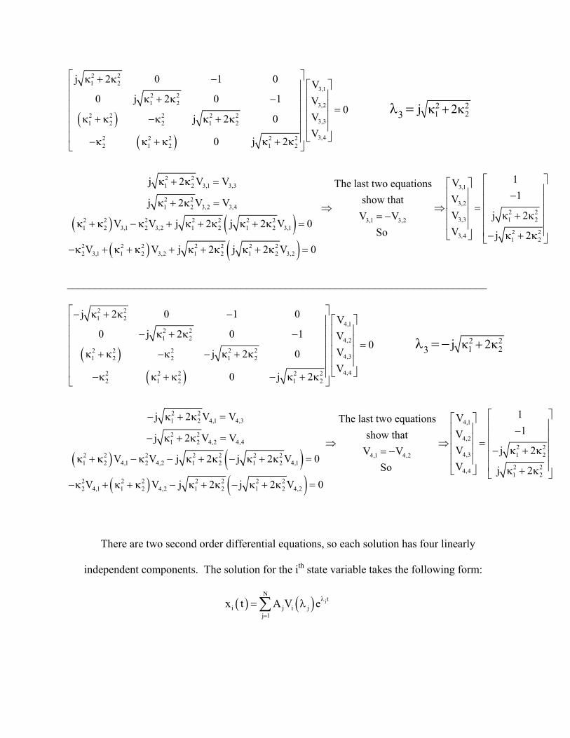
so each solution has four linearly

th state variable takes the following form:

( ) jti jV e

−κ + κ + κ − κ + κ − κ + κ

There are two second order differential equations,

independent components. The solution for the i

( )N

i jj 1

x t A λ

=∑= λ

Where the term ( )i jV λ is the ith component of the eigenvector corresponding to the jth

eigenvalue, each A is an arbitrary constant determined by boundary conditions, and xi(t)

is the ith state variable. Renaming the variables

2 21 1 1 2 2j j and j 2 j± κ = ± ω ± κ + κ = ± ω and using Euler’s Identity ( jφe cosφ jsinφ± = ± ),

the equations of motion can be written as

( ) ( ) ( ) ( ) ( ) ( )( ) ( ) ( ) ( ) ( ) ( )

( ) ( ) ( ) ( ) ( ) ( )( ) ( ) ( ) ( ) ( ) ( )

1 1 1 1 2 2

2 2 1 1 2 2

3 1 1 1 1 1 2 2 2 2

4 2 1 1 1 1 2 2 2 2

x t t A cos t Bsin t Ccos t Dsin t

x t t A cos t Bsin t Ccos t Dsin t

x t t Bcos t Asin t Dcos t Csin t

x t t Bcos t Asin t Dcos t Csin t

= θ = ω + ω + ω + ω

= θ = ω + ω − ω − ω

= θ = ω ω − ω ω + ω ω − ω ω

= θ = ω ω − ω ω − ω ω + ω ω

&

&

To determine the arbitrary constants, four boundary conditions must be known. In the

experiment, the boundary conditions were the initial position and velocity of both

pendulums.

As an example, the following is the deriva

conditions (

tion for the Case (iii), using the initial

) ( ) ( ) ( )1 0 2t 0 1; t 0θ = = θ = θ = 1 2t 0 t 0 0= θ = = θ = =& &

1 2

1 2

1x1(0) = A + C = 1 A = 2

x2(0) = A - C = 0 B = 01x3(0) = B + D = 0 C = 2

x4(0) = B - D = 0 D = 0

ω ω

ω ω

⇒

Substituting the coefficients A, B, C, D

( ) ( )

into our original equations of motion,

( ) ( )

( ) ( ) ( ) ( )

1 1 1 2

2 2 1 2

1x t t [cos t cos t ]21x t t [cos t cos t ]2

= θ = ω + ω

= θ = ω − ω

Using the following trigonometric identities, substitutions can be made to the above:

cos cos 2cos cos2 2

cos cos 2sin sin2 2

α + β α −β⎛ ⎞ ⎛ ⎞α + β = ⎜ ⎟ ⎜ ⎟⎝ ⎠ ⎝ ⎠

α + β α −β⎛ ⎞ ⎛ ⎞α − β = − ⎜ ⎟ ⎜ ⎟⎝ ⎠ ⎝ ⎠

( )

( )

1 2 1 21

1 2 1 22

t cos t cos t2 2

t sin t sin t2 2

ω + ω ω − ω⎛ ⎞ ⎛ ⎞θ = ⎜ ⎟ ⎜ ⎟⎝ ⎠ ⎝ ⎠

ω + ω ω − ω⎛ ⎞ ⎛ ⎞θ = ⎜ ⎟ ⎜ ⎟⎝ ⎠ ⎝ ⎠

Which could further be reduced to

( ) ( ) ( )( ) ( ) ( )

1 a b

2 a b

t cos t cos t

t sin t sin t

θ = ω ω

θ = ω ω

1 2a

a

1 2b

b

2t2 T

2t2 T

ω + ω πω = =

ω − ω πω = =

where the final substitution is changing from

radians to frequencies.

Procedure

up of the experiment, with two masses versity http://www.physics.montana.edu

Figure 2. Diagram showing the setPicture obtained from Montana Uni

e of an apparatus setup as follows: two pendulums of

ded with a metal stand from the same

imately one-third length from their tops by a

then connected to sensors at the top of each pendulum to

The analysis involved the us

identical material and dimensions were suspen

height and then connected together at approx

spring. An oscilloscope was

record their respective motion.

k

m m

r

L

θ θ 1

2

Figure 3. Diagram showing the setup of the experiment, with two masses

Image obtained from Prof. Molter

With this apparatus, data was collected with the oscilloscope for the motion of the two

pendulums under three different sets of initial conditions. Before each collection of data,

it was verified that the pendulums were as stationary as possible.

In the first case, both pendulum

that the values of

s were lifted to a higher height and held still so

θ 1 and θ 2 were equivalen

condition ( ) ( )

t. Mathematically, this satisfied the initial

( ) ( )1 2t 0 t 0 0θ = = θ = =& & . Both pendulums

rom the oscilloscope was recorded. This

s lifted to a certain value of

1 2 0t 0 t 0 1;θ = = θ = = θ =

were then released simultaneously, and data f

process was repeated for three trials.

In the second case, one pendulum wa θ 1 and the

agnitude of second pendulum was lifted to the same m θ 1 but in the opposing direction,

mathematically represented as ( ) ( ) ( ) ( )1 2 0 1 2t 0 1; t 0 t 0 0−θ = = θ = θ = = θ = =& & .

ondition were collected after the pendulums

t 0θ = =

Again, data for three trials with this initial c

were released.

In the third and final case, only one pendulum was lifted to a new height with

valueθ 1 while the second pendulum was kept in the neutral position, written as

( ) ( ) ( ) ( )1 0 2 1 2t 0 1; t 0 t 0 t 0 0θ = = θ = θ = = θ = = θ = =& & .

Three trials of data were collected for this initial condition and the subsequent motion of

the pendulums after the single pendulum was released.

The spring constant, necessary for establishing the equations of motion, was also

calculated by first measuring the weight and length of the spring and the force exerted on

the spring by an attached mass, and then applying the equation F = k∆x.

Results

The following initial conditions were exam

Case 1: Both pendulums were pushed in the sam

(as observed by the output on the osc

Case 2: Both pendulums were pushed outward in

same angle, and released simultaneously.

Case 3: One pendulum was pushed out at and

stationary.

ined:

e direction with the same angle

illoscope) and then simultaneously released.

the opposite direction, but at the

angle while the other remained

The following demonstrates graphs obtained by three different methods:

1) Experimental: As the pendulum moved, the changing resistance of the

potentiometer attached to the pivot caused variations in voltage, which were read

by the two channels of the oscilloscope. The data were extracted using Excel’s

Agilent function, imported into Matlab, and plotted.

2) Simulink: A model (shown under Discussion, Figure 4) was made using

Matlab’s Simulink platform, and the output was saved into two .mat data files

which were then plotted for the appropriate time period to make comparisons

easier.

3) Theoretical: The equations of motion developed in the theory section were

plotted for each case.

The following tabulates the parameters and

Table 1. Measurements of mass and length

measurements used in this experiment.

Mass 1 (kg) 1.5435 Mass 2 (kg) 1.5292 Average mass (kg) 1.5360 Length of rod (m) 0.5950 Distance btw. Pivot and spring on rod 1 (m)

0.1000

Distance btw. Pivot and spring on rod 2 (m)

0.0850

Average length (m) 0.0925

Table 2. Measurements for spring constant Actual weight of spring (kg) 0.01321 Unstretched spring (m) 0.336 Stretched spring (m) 0.368 Measurement 1 ∆x (m) 0.032 Mass applied – weight of spring (kg): 0.10000 – 0.01321 = 0.08679 Corresponding force (N) 0.85088 Stretched spring (m) 0.409 Measurement 2 ∆x (m) 0.073 Mass applied – weight of spring (kg): 0.18000 – 0.01321 = 0.16679 Corresponding force (N) 1.63519

Graph 1. Experimental output for case 1.

Note how the waves look very identical, but due to errors and slight differences in release

time, as well as other external factors (see Error Dicussion), the lines do not match as

well as they do in the Simulink or Theoretical graphs.

Graph 2. Experimental output for case 2.

The two waves appear to have the same amplitude and frequency, but are phase shifted

from each other. Note how they begin to dampen after several seconds, due to non-ideal

conditions, including friction and inequalities in weight (see Error Dicussion).

Graph 3. Experimental output for case 3.

Here the discrepancies between the experimental output and the theoretical output are

clear, in that the motion of Mass 2 (which is initially stationary) must increase in

proportion to the decrease in motion of Mass 1, which is released from some angle. In

the theoretical data, the amplitude of Mass 1 does not decrease as quickly, and the

amplitude of Mass 2 increases faster. This discrepancy is caused by factors such as a

spring that is not initially taut, friction, and other details mentioned in Error

Considerations.

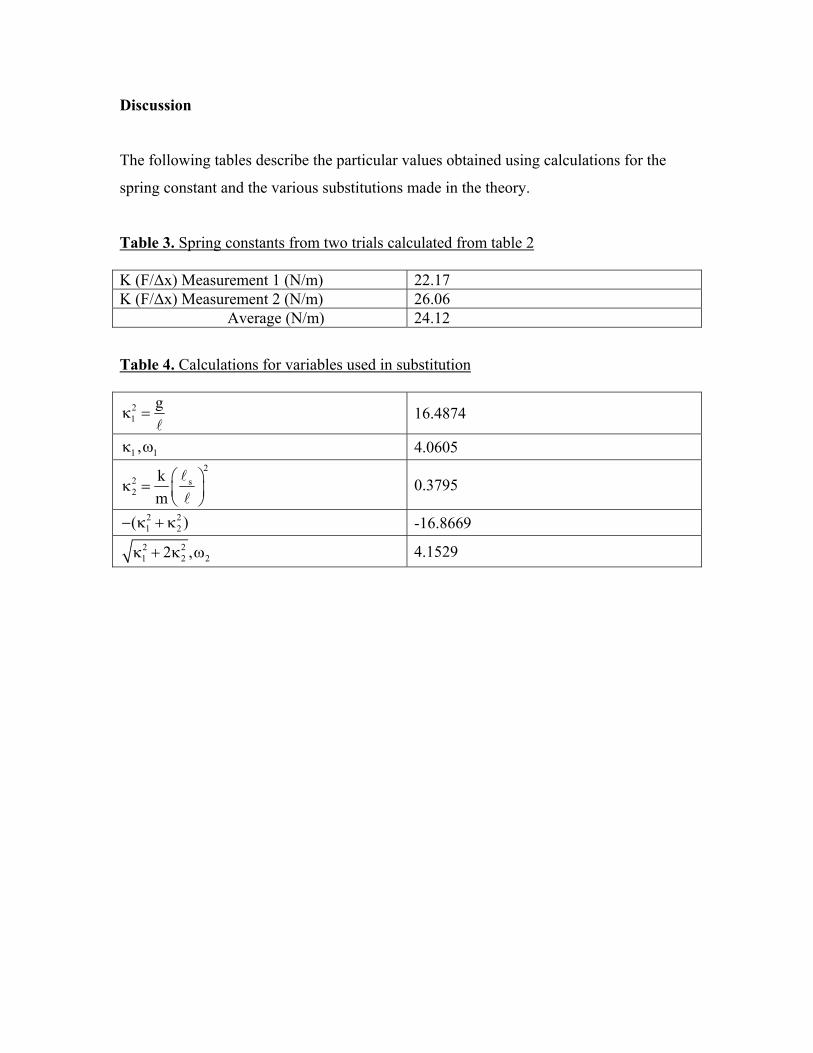
Discussion

The following tables describe the particular values obtained using calculations for the

spring constant and the various substitutions made in the theory.

Table 3. Spring constants from two trials calculated from table 2 K (F/∆x) Measurement 1 (N/m) 22.17 K (F/∆x) Measurement 2 (N/m) 26.06 Average (N/m) 24.12

Table 4. Calculations for variables used in substitution

21

gκ =

l 16.4874

1 1,κ ω 4.0605 2

2 s2

km

⎛ ⎞κ = ⎜ ⎟⎝ ⎠

l

l 0.3795

2 21 2( )− κ + κ -16.8669

2 21 2 22 ,κ + κ ω 4.1529

Graph 4. Theoretical output for case 1.

Note once again that both waves are exactly identical, making them look as one. The

following Matlab code was used for the theoretical form, obtained from the theory:

omega1 = 4.0605 ; t = linspace(0,8) ; y = (cos(omega1*t)) ; z = (cos(omega1*t)) ; plot(t,y, ‘m’, t, z, ‘b :’) title(‘Behavior of case 1 according to equations of motion’) xlabel(‘Time (sec)’) ylabel(‘Angular displacement’) legend(‘Theta1’, ‘Theta2’)

Code 1. Theoretical output for case 1.

Graph 5. Experimental data curve fitted in Kaleidagraph for case 1, x1(t).

We note how the curve fitting is extremely precise and almost super-positioned over the

actual data points.

Graph 6. Experimental data curve fitted in Kaleidagraph for case 1, x2(t).

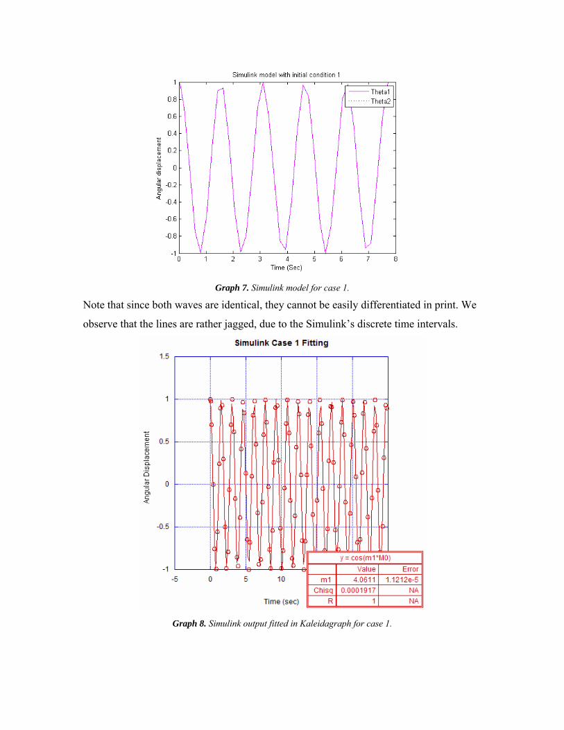
Graph 7. Simulink model for case 1.

Note that since both waves are identical, they cannot be easily differentiated in print. We

observe that the lines are rather jagged, due to the Simulink’s discrete time intervals.

Graph 8. Simulink output fitted in Kaleidagraph for case 1.

Here it can be easily seen that curve-fitting the Simulink results in almost exact fitting,

demonstrating the accuracy of the modeling.

Graph 9. Theoretical output for case 2.

It is clear here that Theta1 is a cosine wave and Theta2 is an inverse cosine wave, as the

theoretical output should be. The following details the Matlab code used for this specific

case.

Omega2 = 4.1529 ; t = linspace(0,8) ; y = (cos(omega2*t)) ; z = -(cos(omega2*t)) ; plot(t,y, ‘m’, t, z, ‘b :’) title(‘Behavior of case 2 according to equations of motion’) xlabel(‘Time (sec)’) ylabel(‘Angular displacement’) legend(‘Theta1’, ‘Theta2’)

Code 2. Theoretical output for case 2.

Graph 10. Experimental data curve fitted in Kaleidagraph for case 2 (for x1(t)- Note how m2 is negative). Curve-fitting the data is slightly more difficult as we see the damping of cosine curve as

the graph progresses. The error, however, is still acceptable.

Graph 11. Experimental data curve fitted in Kaleidagraph for case 2 (for x2(t)- with m1 positive).

Graph 12. Simulink model output for case 2.

Once again it can be seen that the waves are jagged in this Simulink-generated graph.

Graph 13. Simulink model fitted in Kaleidagraph for case 2.

Once again, the curve fitting with the model provided by Simulink is very accurate.

0 5 10 15 20 25 30 35 40 45-1

-0.8

-0.6

-0.4

-0.2

0

0.2

0.4

0.6

0.8

1Behavior of cas e 3 according to equations of motion

Time (s ec)

Ang

ular

dis

plac

emen

t

Theta1Theta2

Graph 14. Theoretical output for case 3.

The following Matlab code was employed to generate the above graph, the theoretical

behavior of the system under initial conditions of case 3.

Omega1 = 4.0605; omega2 = 4.1529; t = [0:.1:45]; y = ½*(cos(omega1*t)+ cos(omega2*t)); z = ½*(cos(omega1*t)- cos(omega2*t)); plot(t,y, ‘m’, t, z, ‘b:’) title(‘Behavior of case 3 according to equations of motion’) xlabel(‘Time (sec)’) ylabel(‘Angular displacement’) legend(‘Theta1’, ‘Theta2’)

Code 3. Theoretical output for case 3.

Graph 15. Kaleidagraph fitting for experimental data, case 3 (Graph for θ1(t), note the positive sign).

Graph 16. Kaleidagraph fitting for experimental data, case 3. (Graph for θ2(t), note the negative sign).

It can be seen that due to the large number of data points Kaleidagraph has difficulty

finding a good curve fit. With appropriate guess values for the curve-fit equation,

however, the generated waveform fits the data points pretty nicely.

Graph 17. Simulink model output for case 3.

Due to the greater time period in which the data was recorded (45 seconds as opposed to

8), the jagged edges seen earlier are less obvious. We see evidence of phrase reversal just

at around the 34-second mark.

Graph 18. Kaleidagraph fitting for Simulink data, case 3 (Graph for θ1(t), note the positive sign).

Graph 19. Kaleidagraph fitting for Simulink data, case 3 (Graph for θ2(t), note the negative sign).

In the above cases, since Simulink’s modeling is undoubtedly accurate, we retain the

generated fitted curve and suggest Kaleidagraph’s attempts at fitting are slightly

inadequate. We do note however that the displayed equation shows a very minimal error,

and ultimately the frequency values are almost identical to the theoretical values. Table 5. Results of values for ω for Experimental, Simulink and Theoretical curve fits

Case, ω1/ ω2 Experimental Simulink Theoretical

Case 1, ω1 4.3189/4.3015

avg. 4.3102 4.0611 4.0605

Case 2, ω2 4.5528/4.4092

avg. 4.4810 4.1535 4.1529

Case 3, ω1 4.2003/4.1001

avg. 4.1502 4.0611/4.061 avg. 4.0611 4.0605

Case 3, ω2 4.279/4.1957 avg. 4.2374

4.1535/4.1535 avg. 4.1535 4.1529

Average ω1 4.2302 4.0611 Average ω2 4.3592 4.1535

Table 6. Error values for each of the above cases

Case, ω1/ ω2 Experimental Simulink Case 1, ω1 6.15% 0.01% Case 2, ω2 7.90% 0.01% Case 3, ω1 2.21% 0.01% Case 3, ω2 2.04% 0.01% Average ω1 4.18% 0.01% Average ω2 4.97% 0.01%

Graph 20. Theoretical output for case 3 using MacOSX Grapher.

The theoretical equations have been plotted using a different software, namely MacOS’s

Grapher. This shows a longer time span. Again, there is a phase reversal at 34 seconds.

The following code reads the Excel file containing the data points read by the Agilent

function, extracts the necessary columns, and plots it with a label, legend, and title.

data=xlsread('H:\E12 Lab 3\Case1Data.xls'); t=data(:,1); c1=data(:,2); c2=data(:,3); plot(t,c1,'b:',t,c2,'m-') title('Oscilloscope output for case 1'); ylabel('Scope Data (Volts)'); xlabel('Time (Sec)'); legend('Input','Output')

Code 4. Matlab code used to import Excel data sheet and graphing them using separate markers and a legend.

Simulink Block diagram

The following diagram was constructed with Matlab’s Simulink program based on the

equations of motion as defined in theory.

Figure 4. Simulink block diagram for coupled pendulums.

Each case was defined by values placed with each of the gains, and where the summing

block required a difference, the gain was made into a negative number. The diagram has

been annotated with the variables from the equations of motion. The following Matlab

code imports data from the outputs of the above block diagram (Theta1.mat and

Theta2.mat), and plots it in the relevant time period (for easy comparison to our

experimental data), adding labels for both the x- and y-axis and adds a legend.

load Theta1 load Theta2 plot(Theta2(1,1:44), Theta2(2,1:44), 'm') hold on plot(Theta1(1,1:44),Theta1(2,1:44), 'b:'); title('Simulink model with initial condition 2'); hold off legend('Theta1', 'Theta2') ylabel('Angular displacement'); xlabel('Time (Sec)');

Code 5. Matlab code for importing data from Simulink and plotting.

Error Discussion

This lab required many assumptions to be made, and as a result undoubtedly contributed

many sources of error, both systematic and random, only some of which are noted here.

1) Our calculations for the pendulums assumed a massless rod. In reality, our rod

had some amount of weight that contributed to the overall behavior of the

pendulums.

2) The pivot was considered to be frictionless. The ball bearings inside, though

coated in a thin layer of oil, no doubt provide unavoidable amounts of friction,

reducing the effect of the springs. Furthermore, the attachment of the transducer

(in the form of a potentiometer, to measure the movement of the pendulum) added

significant friction.

3) The properties of the spring. The spring was considerably longer than the span

that separated both pendulums, and thus its effect was only limited to the cases

where the pendulums’ initial positions forced the spring to be taut. For example,

in case 1 with both pendulums at a same angle in the same direction, the spring’s

effect was minimal in maintaining the distance between the two springs,

whereupon using a spring that was exactly the distance that spanned the two

pendulums would have had a more significant effect. In addition, the spring was

an extension spring, so it never exerted an outward force, although this force was

assumed in the theoretical calculations.

4) The spring might have already suffered a strain on its elastic limit. As we

were the last group to perform this experiment, it is more than likely that the

spring was extended beyond its original state, lending itself to systematic error.

5) The distance between the pivot and the spring was not identical for both

pendulums. As such, calculations made in this experiment employed an average

of the two distances, although the difference ultimately means there was uneven

application of the torque by the spring on the rod.

6) The masses were not identical. Once again, the assumptions made in the lab

were that both masses were the same. The fact that they were not, and the

approximation made in the calculations using the average mass, was likely to

cause errors.

7) Random error in release of pendulums. No mechanical or systematic method

was used to release the pendulums, except the precaution that one person should

release both pendulums at the same time (since it would be nearly impossible for

two people to let go of two different pendulums at the same time). The angle at

which they were released was also only ‘measured’ by the output shown on the

oscilloscope due to the transducer connected to the pivot.

8) The measurement of the spring constant. It was decided upon that the spring

constant would be measured using a spring scale, which unfortunately added more

sources of error, rather than minimize them, since the spring inside the spring

scale had an effect on the overall measurement.

9) The small angle approximation. In the theoretical derivations, it was assumed

that the pendulums would rotate through small enough angles that sinθ=θ and

cosθ=1. However, in some trials, especially for case 3, the pendulums swung

through large enough angles that the small angle approximation would add

considerable error.

Conclusions

In this experiment, a system of two pendulums attached with a spring was

examined. It was analyzed theoretically using free body diagrams to find a set of

differential equations. These equations were solved using the state variable method. The

solutions for the differential equations agreed with the experimental results within 8%

error. The average angular frequency obtained for pendulum 1 was 4.2302 radians, and

was 4.3592 for pendulum 2. The spring used for the experiment was found to have a

spring constant K value of 24.12.

Future Work

Improvements that could have been made on this lab are numerous. An alternative

system could be built, with the same exact distance from the pivots to the spring, and a

better, newer spring with a span identical to the distance between the pivots could be

used. Also, a spring that exerts a force when compressed should be used. The masses that

are suspended beneath can also be modified so that they are the same. A mechanical

device could be employed to hold both masses at the same time and let go at a defined

moment. Also, lower friction in the pivot would help greatly.

Different forms of the same lab could also be performed, including using springs

with different spring constants, rods of different length, masses of different weight, and a

comparison of the system’s behavior with different initial angular displacements. Another

interesting comparison would be to conduct experiments with the spring further below

the pivot. In the place of a spring, a cord or rope could be used, and the results could

reveal their behavior under tension.

With this experiment, however, it might have helped to pay a little more careful

attention to minute details in order to minimize the errors encountered, even though such

errors were present irregardless. For example, the measurement of the spring constant

could have been done with a known (or measured) weight suspended from the spring

itself (rather than a spring scale, which adds another factor of error). It did help however

to conduct multiple trials of the same step, so that the best (or the average) measurement

could be used for the experiment.

Bibliography

Moreshet, Tali. Laboratory 3: Coupled Pendula System

<http://www.swarthmore.edu/NatSci/tali/E12/E12.07.Lab3.Coupled.Pendulum.doc>

Acknowledgements

Grateful acknowledgement is made to Prof. Moreshet for guidance in initial calculations

and theory for the experiment.