
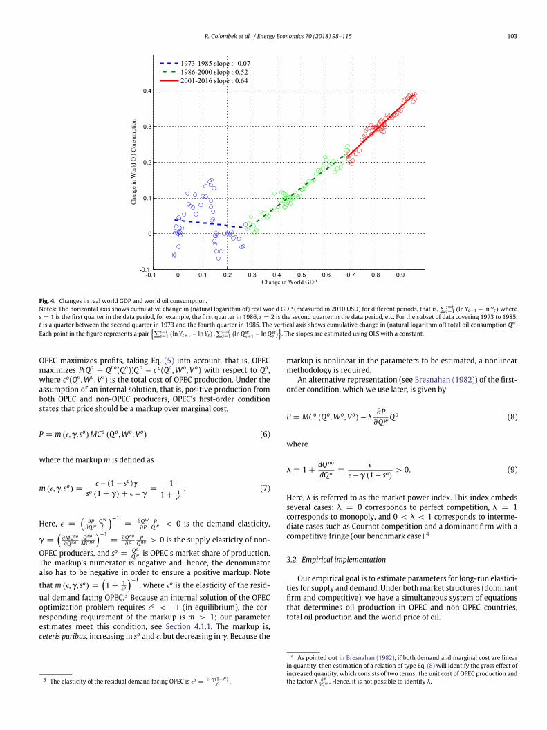
EnergyEconomics OPEC’smarketpower ...(b) World Oil Consumption and Non−OPEC Production total...
18
Energy Economics 70 (2018) 98–115 Contents lists available at ScienceDirect Energy Economics journal homepage: www.elsevier.com/locate/eneco OPEC’s market power: An empirical dominant firm model for the oil market Rolf Golombek a, * , Alfonso A. Irarrazabal b , Lin Ma c a Ragnar Frisch Centre for Economic Research, Norway b Norwegian Business School, Norway c School of Economics and Business, Norwegian University of Life Sciences (NMBU), Norway ARTICLE INFO Article history: Received 30 September 2016 Received in revised form 8 November 2017 Accepted 12 November 2017 Available online xxxx JEL classification: L13 L22 Q31 Keywords: Oil Dominant firm Market power OPEC Lerner index Oil demand elasticity Oil supply elasticity ABSTRACT We estimate a dominant firm-competitive fringe model for the crude oil market using quarterly data on oil prices for the 1986–2016 period. The estimated structural parameters have the expected signs and are significant. We find that OPEC exercised market power during the sample period. Counterfactual experiments indicate that world GDP is the main driver of long-run oil prices. However, supply (depletion) factors have become more important in recent years. © 2017 The Authors. Published by Elsevier B.V. This is an open access article under the CC BY-NC-ND license (http://creativecommons.org/licenses/by-nc-nd/4.0/) 1. Introduction Oil prices have changed substantially over the last three decades. Researchers have considered many explanations to account for the long-run behavior of prices, including growing demand from emerging economies, noncompetitive behavior of OPEC, resource depletion, and rising extraction costs. To understand which factors are paramount in driving the oil price, estimation of cost and demand parameters under different market structures is required. Because supply relations and demand function are likely to move simultaneously as a result of exogenous shifters (such as income and technological factors), econometric methods such as instrumental variables should be used to estimate these parameters. * Corresponding author at: Frisch Centre Forskningsparken Gaustadalleen 21, Oslo 0349, Norway. E-mail addresses: [email protected] (R. Golombek), [email protected] (A.A. Irarrazabal), [email protected] (L. Ma). Unfortunately, the application of these methods to the oil market has proven difficult, see Hamilton (2009). We use the dominant firm-competitive fringe textbook model (OPEC versus the group of non-OPEC producers) and estimate significant elasticities over the sample period, 1986–2016. The simultaneity bias is corrected for by using standard instrumental variable (IV) methods. We show that it is critical to correctly specify the market structure to obtain significant elasticities, and document that OPEC exercised market power during the sample period, 1986– 2016. In our model, demand is standard — it depends on the current oil price and world GDP — but we depart from standard supply analysis by assuming that one group of oil producers, OPEC, can exert market power, whereas the non-OPEC oil producers act as a com- petitive fringe. Once OPEC sets the price of oil, total demand and the fringe’s supply are determined, and OPEC is faced with the residual demand: total demand less the competitive supply. OPEC sets the price that maximizes its total profits, taking into account the impact of its pricing decision on the residual demand. This choice leads to a nonlinear price-setting rule. https://doi.org/10.1016/j.eneco.2017.11.009 0140-9883/© 2017 The Authors. Published by Elsevier B.V. This is an open access article under the CC BY-NC-ND license (http://creativecommons.org/licenses/by-nc-nd/4.0/)
Transcript of EnergyEconomics OPEC’smarketpower ...(b) World Oil Consumption and Non−OPEC Production total...

Energy Economics 70 (2018) 98–115
Contents lists available at ScienceDirect
Energy Economics
j ourna l homepage: www.e lsev ie r .com/ locate /eneco
OPEC’s market power: An empirical dominant firm model forthe oil market
Rolf Golombeka,*, Alfonso A. Irarrazabalb, Lin Mac
a Ragnar Frisch Centre for Economic Research, Norwayb Norwegian Business School, Norwayc School of Economics and Business, Norwegian University of Life Sciences (NMBU), Norway
A R T I C L E I N F O
Article history:Received 30 September 2016Received in revised form 8 November 2017Accepted 12 November 2017Available online xxxx
JEL classification:L13L22Q31
Keywords:OilDominant firmMarket powerOPECLerner indexOil demand elasticityOil supply elasticity
A B S T R A C T
We estimate a dominant firm-competitive fringe model for the crude oil market using quarterly dataon oil prices for the 1986–2016 period. The estimated structural parameters have the expected signsand are significant. We find that OPEC exercised market power during the sample period. Counterfactualexperiments indicate that world GDP is the main driver of long-run oil prices. However, supply (depletion)factors have become more important in recent years.
© 2017 The Authors. Published by Elsevier B.V. This is an open access article under the CC BY-NC-NDlicense (http://creativecommons.org/licenses/by-nc-nd/4.0/)
1. Introduction
Oil prices have changed substantially over the last three decades.Researchers have considered many explanations to account forthe long-run behavior of prices, including growing demand fromemerging economies, noncompetitive behavior of OPEC, resourcedepletion, and rising extraction costs. To understand which factorsare paramount in driving the oil price, estimation of cost anddemand parameters under different market structures is required.Because supply relations and demand function are likely tomove simultaneously as a result of exogenous shifters (such asincome and technological factors), econometric methods such asinstrumental variables should be used to estimate these parameters.
* Corresponding author at: Frisch Centre Forskningsparken Gaustadalleen 21, Oslo0349, Norway.
E-mail addresses: [email protected] (R. Golombek),[email protected] (A.A. Irarrazabal), [email protected] (L. Ma).
Unfortunately, the application of these methods to the oil market hasproven difficult, see Hamilton (2009).
We use the dominant firm-competitive fringe textbook model(OPEC versus the group of non-OPEC producers) and estimatesignificant elasticities over the sample period, 1986–2016. Thesimultaneity bias is corrected for by using standard instrumentalvariable (IV) methods. We show that it is critical to correctly specifythe market structure to obtain significant elasticities, and documentthat OPEC exercised market power during the sample period, 1986–2016.
In our model, demand is standard — it depends on the currentoil price and world GDP — but we depart from standard supplyanalysis by assuming that one group of oil producers, OPEC, can exertmarket power, whereas the non-OPEC oil producers act as a com-petitive fringe. Once OPEC sets the price of oil, total demand and thefringe’s supply are determined, and OPEC is faced with the residualdemand: total demand less the competitive supply. OPEC sets theprice that maximizes its total profits, taking into account the impactof its pricing decision on the residual demand. This choice leads to anonlinear price-setting rule.
https://doi.org/10.1016/j.eneco.2017.11.0090140-9883/© 2017 The Authors. Published by Elsevier B.V. This is an open access article under the CC BY-NC-ND license (http://creativecommons.org/licenses/by-nc-nd/4.0/)
R. Golombek et al. / Energy Economics 70 (2018) 98–115 99
Our empirical model contains a simultaneous system of threeequations and is estimated using nonlinear instrumental variablemethods with world GDP and production costs for OPEC and non-OPEC producers as exogenous demand and supply shifters. We usequarterly data from 1986 to 2016, which is a period after the majorstructural changes in the oil market in the 1960s and the 1970s. Ourresults suggest that the nonlinearity induced by OPEC’s markup is ofkey importance in modeling oil prices.
We find that the dominant firm model provides a good represen-tation of the oil market: all structural parameters have the expectedsigns and are statistically significant (except for the marginal costelasticity of OPEC). We estimate a long-run price elasticity ofdemand of −0.35, which is somewhat larger than previous estimatesreported in the literature (see, for example, Dahl, 1993; Gately andHuntington, 2002; and Cooper, 2003). Our estimate of the incomeelasticity of demand is 1.15, which is higher than previous estimates,see, for example, the Gately and Huntington (2002) study (0.55 forOECD countries and 1.17 for non-OECD countries including Chinaand India) and Graham and Glaister (2004). We believe our resultsreflect that China and India, which had high GDP growth rates in thedata period, 1986–2016, had high income elasticities in this period.
We find a non-OPEC supply elasticity of 0.32. Because the demandand non-OPEC supply elasticities are statistically significant, weobtain a tight estimate for the degree of OPEC’s market power —we find evidence that OPEC exerted substantial market power in theperiod analyzed.
To gain insight about the role of OPEC’s markup for our empiricalresults, we reestimate the model under the assumption that OPEC is aprice taker. With a competitive model we obtain an insignificant (andmarginally positive) demand elasticity — a similar result has beenobtained in some previous studies, such as Lin (2011). Using the com-petitive model, we also obtain a lower income elasticity (around 0.5)and find an insignificant factor price elasticity for OPEC. The differ-ence between the results obtained from the competitive model andthe dominant firm model reflects the nonlinear response induced byOPEC’s markup on its residual demand. In our model, OPEC’s markupis not a constant; it is a function of parameters (to be estimated) andendogenous variables.
Using our estimates, we examine the contribution of world GDPand production costs to the long-run trend in oil prices and quan-tities during our sample period from 1986 to 2016. We find thatchanges in world GDP explain most of the growth in oil prices andquantities, but the recent rise in production costs is also responsiblefor higher prices after 2005.
We make four contributions to the literature on crude oil prices.First, there is a large literature on estimating the relationshipbetween oil demand and the price of oil, and also the relationshipbetween supply of oil and the price of oil (see, for example, Griffin,1985, Kaufmann, 2004, Kaufmann et al., 2008 and Brémond et al.,2012). These papers do not account for the simultaneity of supply-and-demand changes. Hamilton (2009) argues that, for some periods,these estimates are probably good approximations, but, in general,they are subject to instabilities. Studies that have taken the simul-taneity of supply-and-demand changes into account, as we do, arescarce — some examples are Alhajji and Huettner (2000), Krichene(2002), Almoguera et al. (2011), and Lin (2011). We contribute to thisliterature by estimating a simultaneous dominant firm-competitivefringe model for the oil market, using the nonlinear instrumentalvariable method — the nonlinear estimator reflects the nonlinear-ity of the system of equations to be estimated.We obtain statisticallysignificant demand and fringe (non-OPEC) supply elasticities.
Second, our paper is related to the literature that tests the degreeto which OPEC can control prices. Griffin (1985) is a seminal paper inthis field. In testing whether OPEC is a cartel, Griffin starts out assum-ing that OPEC is a dominant firm that sets the price of oil. However,the residual demand function, as well as a first-order condition for
OPEC, are not part of the empirical model. Alhajji and Huettner(2000) and Hansen and Lindholt (2008) also refer to the dominantfirm model, but, again, OPEC’s price-setting rule is not part of theempirical model in these papers. To the best of our knowledge, thepresent paper is the first to estimate the simultaneous dominant firmmodel for the oil market.
Whereas Griffin (1985) concludes that most OPEC countries act asmembers of a cartel, evidence of OPEC’s ability to influence the priceof oil is mixed. Papers in the 1980s and 1990s argued in favor of col-lusive behavior, see, for example, Almoguera et al. (2011), but laterstudies, using extended data, found mixed evidence of whether OPEChas exerted market power. For example, Spilimbergo (2001) findsno support for the hypothesis that OPEC, except for Saudi Arabia,was a market-sharing cartel during the 1983–1991 period, whereasSmith (2005) finds that OPEC’s market behavior lies between a non-cooperative oligopoly and a cartel. Boug et al. (2016) present a modelthat encompasses several alternative specifications suggested in theliterature. They find support for imperfect competition in the oilmarket, and also that OPEC’s behavior has changed significantly overthe last years. For other studies, see Jones (1990), Gulen (1996),Brémond et al. (2012), Cairns and Calfucura (2012), Huppmann andHolz (2012), Colgan (2014), Kisswani (2016) and Okullo and Reynès(2016). Smith (2009) and Fattouh and Mahadeva (2013) presentreviews of the literature. Our contribution is to test whether OPEChad market power by using a non-nested statistical test for com-peting models: by comparing our dominant firm model with thecompetitive model, we find no evidence to reject the dominant firmmodel.
Third, using the model’s estimated parameters, we show thatgrowth in world GDP has been the main driving force of oil priceincreases over the last three decades, but recent rises in productioncosts have contributed significantly to higher oil prices. To the bestof our knowledge, we are among the first to document the relativeimportance of demand and supply factors for the long-run behavior ofoil prices, see Section 4.2. In contrast, some studies, like Kilian (2009),assume that supply is fixed, which is reasonable in the short run.
Finally, our paper complements results from the empirical indus-trial organization literature on measuring the degree of marketpower, see, for example, Suslow (1986), which finds substantial mar-ket power in the aluminum industry in the period between WorldWar I and World War II. Our measure of market power builds onBresnahan (1982), and, as reported above, we find clear evidence ofexertion of market power in the oil market between 1986 and 2016.For a survey of the literature on industries with market power, seeBresnahan (1989).
Our paper is divided into six sections. In Section 2, we provide anoverview of the crude oil market, and, in Section 3, we describe theempirical framework used to estimate the model. The main resultsare presented in Section 4. Here, we compare our estimated elastic-ities with those reported in the literature and discuss the fit of themodel. We also analyze the relative importance of world income andcosts of extraction as the driving forces of the oil price. In Section 5,we perform a number of robustness checks. Section 6 concludes.
2. The crude oil market
In this section, we describe the data sources and characterizethe crude oil market, focusing on the period that is analyzed in thispaper.
2.1. Data
We use quarterly data for the period, 1986:Q1–2016:Q4. Theprice of crude oil is measured by the West Texas Intermediate (WTI),which we obtained from the Federal Reserve Bank of St. Louis (2017).
100 R. Golombek et al. / Energy Economics 70 (2018) 98–115
Nominal prices are deflated by the US CPI, see U.S. Bureau of LaborStatistics (2017a). Data on oil production and inventory of crude oilin OECD countries were obtained from EIA (2017). World productionof crude oil plus the change in the OECD inventory of crude oil is usedas a measure for total consumption of (demand for) crude oil.1
Our data on OPEC’s production costs combine annual data (forthe period, 1986–2000) in Hansen and Lindholt (2008) and quarterlydata (for the period, 2001–2016) from IHS CERA. Both series covercosts of exploration, development and production. For non-OPECproduction costs, we use US costs of oil production, which webelieve is a conservative estimate: among the non-OPEC producers,US producers have the highest cost, see Alhajji and Huettner (2000).The source for the non-OPEC cost of production is U.S. Bureau ofLabor Statistics (2017b), which compiles a Producer Price Index (PPI)for oil and gas field machinery and equipment costs in the UnitedStates. We set the nominal production cost for non-OPEC suppliersto 10 dollars per barrel in 1999:Q2 (IHS CERA, 2000).
Like Kaufmann (2004) and Kaufmann et al. (2008), we also usedata for OPEC’s installed extraction capacity; these are obtained fromKaufmann (2005) for the period, 1986:Q1–2007:Q3, and from theIEA Oil Market Report for the period, 2007:Q4–2016:Q4.2 Finally, weused the quarterly world GDP index from Fagan et al. (2001) for theperiod, 1986:Q1–2010:Q4, and Global Financial Data for the period,2011:Q1–2016:Q4. The series is deflated by the US CPI.
2.2. Development in the oil market
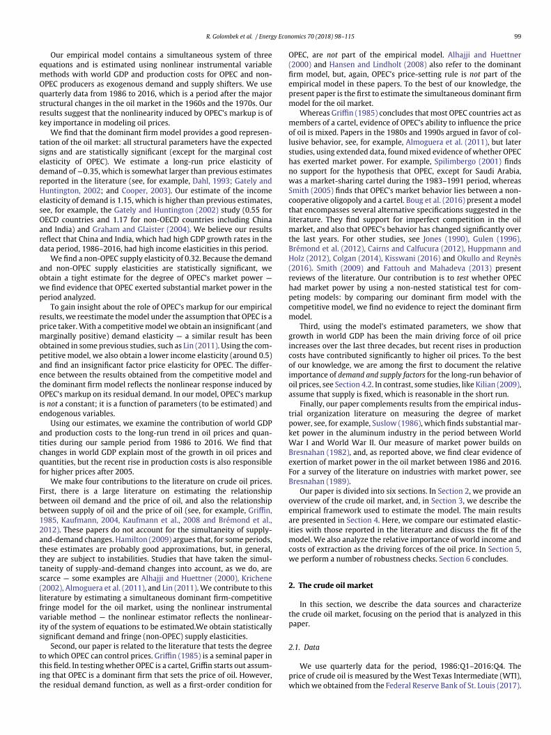
In this subsection, we describe the main development in theglobal oil market since 1973, and also relate this to economicdevelopment. Panel (a) in Fig. 1 plots the real price of oil (measuredin 2010 USD). The figure covers most of the turbulent period between1973 and 1986, encompassing the huge increase in the oil price thatoccurred in 1973 when prices rose from 18 to 52 USD per barrel(frequently referred to as OPEC 1). It also includes the sky-high pricesaround 1979–1980 at roughly 100 USD per barrel (OPEC 2), and thesubstantial decrease in the oil price during the first half of the 1980s.It is beyond the scope of this paper to discuss this early period — theprice path in this period probably reflects structural shocks on thesupply side. Rather, our focus centers on the period after 1985, whichis characterized by less abrupt changes in the crude oil market.
As seen from panel (a), the real oil price was roughly in the rangeof 20 to 40 USD per barrel from 1986 to 1998, except for the peakin 1990:Q3–1991:Q1, a rise that can be attributed to supply disrup-tions stemming from the Gulf War. Beginning in 1999, the oil priceincreased steadily and peaked at 126 USD per barrel in 2008:Q2,then dropped to around 40 USD due to the financial crisis, butincrease again rather rapidly: In 2012–2014, the oil price was close to100 USD. However, late in 2014, the price dropped; it went down toaround 40 USD in 2015–2016.
Panel (b) shows that total production of oil increased steadilyafter 1985. In this period, non-OPEC production did not change much,but there was a drop in production in the early 1990s, reflecting thecontraction of the energy industry in the former Soviet Union. Thetwo plots in panel (b) imply that the OPEC’s market share increased
1 Ideally, we would have used the change in world inventory of crude oil, butwe do not have these data. Because the change in the OECD inventory of crude oilamounts to roughly 1% of world crude oil extraction, we believe our approximationof total demand for crude oil is good. We construct a quarterly data series for worldconsumption of oil, simply because no such series was previously available.
2 Because we have data from both sources for 2007:Q2, we can check the extent towhich the series differ in this quarter. We find that the difference is very small, butwe still use this difference (measured as a percentage) to adjust the Kaufmann et al.(2008) data.
from 30% in 1986 to 40% in 1992 (see Fig. 1 panel (c)), where it hasremained.
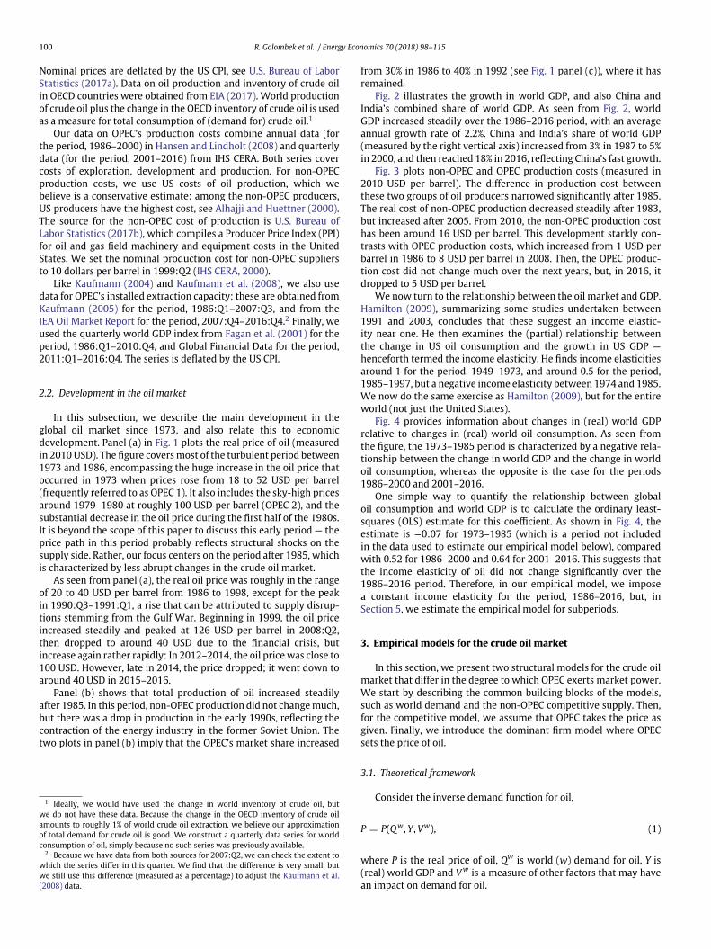
Fig. 2 illustrates the growth in world GDP, and also China andIndia’s combined share of world GDP. As seen from Fig. 2, worldGDP increased steadily over the 1986–2016 period, with an averageannual growth rate of 2.2%. China and India’s share of world GDP(measured by the right vertical axis) increased from 3% in 1987 to 5%in 2000, and then reached 18% in 2016, reflecting China’s fast growth.
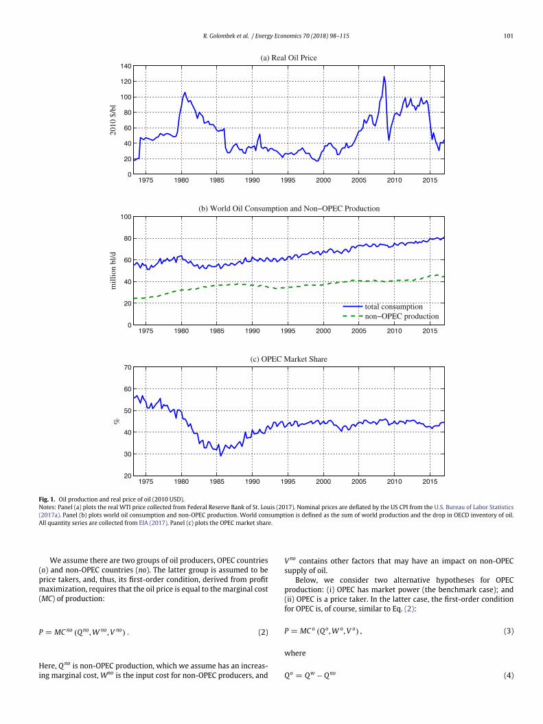
Fig. 3 plots non-OPEC and OPEC production costs (measured in2010 USD per barrel). The difference in production cost betweenthese two groups of oil producers narrowed significantly after 1985.The real cost of non-OPEC production decreased steadily after 1983,but increased after 2005. From 2010, the non-OPEC production costhas been around 16 USD per barrel. This development starkly con-trasts with OPEC production costs, which increased from 1 USD perbarrel in 1986 to 8 USD per barrel in 2008. Then, the OPEC produc-tion cost did not change much over the next years, but, in 2016, itdropped to 5 USD per barrel.
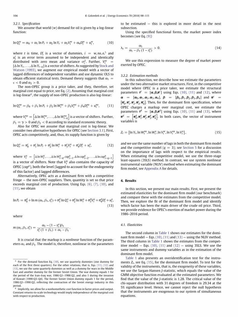
We now turn to the relationship between the oil market and GDP.Hamilton (2009), summarizing some studies undertaken between1991 and 2003, concludes that these suggest an income elastic-ity near one. He then examines the (partial) relationship betweenthe change in US oil consumption and the growth in US GDP —henceforth termed the income elasticity. He finds income elasticitiesaround 1 for the period, 1949–1973, and around 0.5 for the period,1985–1997, but a negative income elasticity between 1974 and 1985.We now do the same exercise as Hamilton (2009), but for the entireworld (not just the United States).
Fig. 4 provides information about changes in (real) world GDPrelative to changes in (real) world oil consumption. As seen fromthe figure, the 1973–1985 period is characterized by a negative rela-tionship between the change in world GDP and the change in worldoil consumption, whereas the opposite is the case for the periods1986–2000 and 2001–2016.
One simple way to quantify the relationship between globaloil consumption and world GDP is to calculate the ordinary least-squares (OLS) estimate for this coefficient. As shown in Fig. 4, theestimate is −0.07 for 1973–1985 (which is a period not includedin the data used to estimate our empirical model below), comparedwith 0.52 for 1986–2000 and 0.64 for 2001–2016. This suggests thatthe income elasticity of oil did not change significantly over the1986–2016 period. Therefore, in our empirical model, we imposea constant income elasticity for the period, 1986–2016, but, inSection 5, we estimate the empirical model for subperiods.
3. Empirical models for the crude oil market
In this section, we present two structural models for the crude oilmarket that differ in the degree to which OPEC exerts market power.We start by describing the common building blocks of the models,such as world demand and the non-OPEC competitive supply. Then,for the competitive model, we assume that OPEC takes the price asgiven. Finally, we introduce the dominant firm model where OPECsets the price of oil.
3.1. Theoretical framework
Consider the inverse demand function for oil,
P = P(Qw, Y , Vw), (1)
where P is the real price of oil, Qw is world (w) demand for oil, Y is(real) world GDP and V w is a measure of other factors that may havean impact on demand for oil.
R. Golombek et al. / Energy Economics 70 (2018) 98–115 101
1975 1980 1985 1990 1995 2000 2005 2010 20150
20
40
60
80
100
120
140(a) Real Oil Price
2010
$/b
l
1975 1980 1985 1990 1995 2000 2005 2010 20150
20
40
60
80
100
mill
ion
bl/d
(b) World Oil Consumption and Non−OPEC Production
total consumptionnon−OPEC production
1975 1980 1985 1990 1995 2000 2005 2010 201520
30
40
50
60
70
%
(c) OPEC Market Share
Fig. 1. Oil production and real price of oil (2010 USD).Notes: Panel (a) plots the real WTI price collected from Federal Reserve Bank of St. Louis (2017). Nominal prices are deflated by the US CPI from the U.S. Bureau of Labor Statistics(2017a). Panel (b) plots world oil consumption and non-OPEC production. World consumption is defined as the sum of world production and the drop in OECD inventory of oil.All quantity series are collected from EIA (2017). Panel (c) plots the OPEC market share.
We assume there are two groups of oil producers, OPEC countries(o) and non-OPEC countries (no). The latter group is assumed to beprice takers, and, thus, its first-order condition, derived from profitmaximization, requires that the oil price is equal to the marginal cost(MC) of production:
P = MC no (Qno, W no, V no) . (2)
Here, Q no is non-OPEC production, which we assume has an increas-ing marginal cost, Wno is the input cost for non-OPEC producers, and
V no contains other factors that may have an impact on non-OPECsupply of oil.
Below, we consider two alternative hypotheses for OPECproduction: (i) OPEC has market power (the benchmark case); and(ii) OPEC is a price taker. In the latter case, the first-order conditionfor OPEC is, of course, similar to Eq. (2):
P = MC o (Qo, W o, V o) , (3)
where
Qo = Qw − Qno (4)
102 R. Golombek et al. / Energy Economics 70 (2018) 98–115
1975 1980 1985 1990 1995 2000 2005 2010 2015
0
50
100
2010
trill
ion
$
1975 1980 1985 1990 1995 2000 2005 2010 20150
10
20
%
Share of World GDP of China and IndiaWorld GDP
Fig. 2. Real world GDP and China and India’s share of world GDP.Notes: The figure plots real world GDP (measured by the left vertical axis in 2010 USD) and China and India’s share of world GDP (measured by the right vertical axis). World GDPis combined using the GDP index from Fagan et al. (2001) for the period 1986–2010 and Global Financial Data (2017) for the period 2011–2016.
is OPEC production(
∂MCo
∂Qo > 0)
. Alternatively, OPEC is not a price
taker. This hypothesis takes into consideration that OPEC’s produc-tion has an impact on the price of oil: if OPEC production increases,then, ceteris paribus, the price of oil will decrease, and, therefore,non-OPEC extraction will decrease. Formally, Eq. (2) can be rewritten
as P(Qo + Q no) = MC no(Q no, W no, V no), which implicitly defines thefunction Qno = Q no(Qo) where
dQno
dQo = −∂P
∂Qw
∂P∂Qw − ∂MCno
∂Qno
< 0. (5)
1975 1980 1985 1990 1995 2000 2005 2010 20150
5
10
15
20
25
2010
$/b
l
Non-OPECOPEC
Fig. 3. Real cost of production in OPEC and non-OPEC.Notes: The OPEC cost series is annual cost of OPEC for 1975–2000 in Hansen and Lindholt (2008) and quarterly observations of costs of exploration, development and productionfor 2001:Q1–2016:Q4 from IHS CERA. The source for the non-OPEC cost is U.S. Bureau of Labor Statistics (2017b). It is a Producer Price Index for oil and gas field machinery andequipment in the United States. We set the nominal cost for non-OPEC to 10 USD per barrel in 1999:Q2 (IHS CERA, 2000).
R. Golombek et al. / Energy Economics 70 (2018) 98–115 103
-0.1 0 0.1 0.2 0.3 0.4 0.5 0.6 0.7 0.8 0.9-0.1
0
0.1
0.2
0.3
0.4
Cha
nge
in W
orld
Oil
Con
sum
ptio
n
Change in World GDP
1973-1985 slope : -0.071986-2000 slope : 0.522001-2016 slope : 0.64
Fig. 4. Changes in real world GDP and world oil consumption.Notes: The horizontal axis shows cumulative change in (natural logarithm of) real world GDP (measured in 2010 USD) for different periods, that is,
∑s=ts=1 (ln Ys+1 − ln Ys) where
s = 1 is the first quarter in the data period, for example, the first quarter in 1986, s = 2 is the second quarter in the data period, etc. For the subset of data covering 1973 to 1985,t is a quarter between the second quarter in 1973 and the fourth quarter in 1985. The vertical axis shows cumulative change in (natural logarithm of) total oil consumption Qw .Each point in the figure represents a pair
{∑s=ts=1 (ln Ys+1 − ln Ys) ,
∑s=ts=1
(ln Qw
s+1 − ln Qws
)}. The slopes are estimated using OLS with a constant.
OPEC maximizes profits, taking Eq. (5) into account, that is, OPECmaximizes P(Qo + Qno(Qo))Q o − c o(Qo, W o, V o) with respect to Qo,where co(Qo, Wo, Vo) is the total cost of OPEC production. Under theassumption of an internal solution, that is, positive production fromboth OPEC and non-OPEC producers, OPEC’s first-order conditionstates that price should be a markup over marginal cost,
P = m (4,c, so) MCo (Qo, Wo, Vo) (6)
where the markup m is defined as
m (4,c, so) =4 − (1 − so)c
so (1 + c) + 4 − c=
1
1 + 14o
. (7)
Here, 4 =(
∂P∂Qw
Qw
P
)−1= ∂Qw
∂PP
Qw < 0 is the demand elasticity,
c =(
∂MCno
∂QnoQno
MC no
)−1= ∂Qno
∂PP
Qno > 0 is the supply elasticity of non-
OPEC producers, and so = Qo
Qw is OPEC’s market share of production.The markup’s numerator is negative and, hence, the denominatoralso has to be negative in order to ensure a positive markup. Note
that m (4,c, so) =(
1 + 14o
)−1, where 4o is the elasticity of the resid-
ual demand facing OPEC.3 Because an internal solution of the OPECoptimization problem requires 4o < −1 (in equilibrium), the cor-responding requirement of the markup is m > 1; our parameterestimates meet this condition, see Section 4.1.1. The markup is,ceteris paribus, increasing in so and 4, but decreasing in c. Because the
3 The elasticity of the residual demand facing OPEC is 4o = 4−c(1−so)so .
markup is nonlinear in the parameters to be estimated, a nonlinearmethodology is required.
An alternative representation (see Bresnahan (1982)) of the first-order condition, which we use later, is given by
P = MCo (Qo, Wo, Vo) − k∂P
∂Qw Qo (8)
where
k = 1 +dQno
dQo =4
4 − c (1 − so)> 0. (9)
Here, k is referred to as the market power index. This index embedsseveral cases: k = 0 corresponds to perfect competition, k = 1corresponds to monopoly, and 0 < k < 1 corresponds to interme-diate cases such as Cournot competition and a dominant firm with acompetitive fringe (our benchmark case).4
3.2. Empirical implementation
Our empirical goal is to estimate parameters for long-run elastici-ties for supply and demand. Under both market structures (dominantfirm and competitive), we have a simultaneous system of equationsthat determines oil production in OPEC and non-OPEC countries,total oil production and the world price of oil.
4 As pointed out in Bresnahan (1982), if both demand and marginal cost are linearin quantity, then estimation of a relation of type Eq. (8) will identify the gross effect ofincreased quantity, which consists of two terms: the unit cost of OPEC production andthe factor k ∂P
∂Qw . Hence, it is not possible to identify k.
104 R. Golombek et al. / Energy Economics 70 (2018) 98–115
3.2.1. SpecificationWe assume that world (w) demand for oil is given by a log-linear
function:
ln Qwt = a0 + a1 ln Pt + a2 ln Yt + a3Vw
t + a4Dwt + uw
t , (10)
where t is time, Dit is a vector of dummies, i = w, no, o,5 and
uit is an error term assumed to be independent and identically
distributed with zero mean and variance s2i . Further, Vw
t =[D ln Yt , . . . ,D ln Yt−q] is a vector of shifters. As suggested by Stock andWatson (1993), we augment our empirical model with a vector oflagged differences of independent variables and use dynamic OLS toobtain efficient statistical tests. Demand theory suggests that a1 =4 < 0 and a2 > 0.
The non-OPEC group is a price taker, and they, therefore, setmarginal cost equal to price, see Eq. (2). Assuming that marginal costis log-linear6, the supply of non-OPEC production is also log-linear:
ln Qnot = b0 + b1 ln Pt + b2 ln Wno
t + b3Vnot + b4Dno
t + unot , (11)
where Vnot =
[D ln Wno
t , . . . ,D ln Wnot−q
]is a vector of shifters. Further,
b1 = c > 0 and b2 < 0 according to standard economic theory.Also for OPEC we assume that marginal cost is log-linear. We
consider two alternative hypotheses for OPEC (see Section 3.1). First,OPEC acts competitively, and, thus, its supply function is given by
ln Qot = pc
0 + pc1 ln Pt + pc
2 ln Wot + pc
3Vot + pc
4Dot + uo
t , (12)
where Vot =
[D ln Wo
t , . . . ,D ln Wot−q , capo
t−1,D ln capot−2, . . . ,D ln capo
t−q−1
]is a vector of shifters. Note that Vo
t also contains the capacity ofOPEC (capo), both the level (lagged to account for the endogeneityof this factor) and lagged differences.
Alternatively, OPEC acts as a dominant firm with a competitivefringe — the non-OPEC suppliers. Then, quantity is set so that priceexceeds marginal cost of production. Using Eqs. (6), (7), (10), and(11), we obtain
ln Pt = pd0 +ln m (a1,b1, so
t )+pd1 ln Qo
t +pd2 ln Wo
t +pd3Vo
t +pd4Do
t +uot ,
(13)
where
m (a1,b1, sot ) =
a1 − (1 − sot )b1
sot (1 + b1) + a1 − b1
.
It is crucial that the markup is a nonlinear function of the param-eters a1 and b1. The model is, therefore, nonlinear in the parameters
5 For the demand function Eq. (10), we use quarterly dummies (one dummy foreach of the first three quarters). For the other relations, that is, Eqs. (11), (12) and(13), we use the same quarterly dummies as well as a dummy for wars in the MiddleEast and another dummy for the former Soviet Union. The war dummy equals 1 forthe period of the Iran–Iraq war, 1986:Q1–1988:Q2, and also 1 during the invasionof Kuwait (1990:Q3–Q4). The former Soviet Union dummy equals 1 for the period,1986:Q1–1990:Q2, reflecting the contraction of the Soviet energy industry in thisperiod.
6 Implicitly, we allow for a nonhomothetic cost function in factor prices and output.Constant returns-to-scale technology would imply independence of the marginal costwith respect to production.
to be estimated — this is explored in more detail in the nextsubsection.
Using the specified functional forms, the market power indexbecomes (see Eq. (9))
kt =a1
a1 − b1 (1 − sot )
> 0. (14)
We use this expression to measure the degree of market powerexerted by OPEC.
3.2.2. Estimation methodsIn this subsection, we describe how we estimate the parameters
under the two alternative market structures. First, in the competitivemodel where OPEC is a price taker, we estimate the structuralparameters hc = [a,b,pc] using Eqs. (10), (11) and (12), where
a = [a0,a1,a2,a3,a4], b = [b0,b1,b2,b3,b4] and pc =[pc
0, pc1, pc
2, pc3,pc
4
]. Then, for the dominant firm specification, where
OPEC charges a markup over marginal cost, we estimate theparameters hd = [a,b,pd] using Eqs. (10), (11) and (13), where
pd =[pd
0, pd1, pd
2, pd3, pd
4
]. In both cases, the vector of instrument
variables is
Zt =[ln Yt , ln Wno
t , ln Wot , ln Vw
t , ln Vnot , ln Vo
t]
, (15)
and we use the same number of lags in both the dominant firm modeland the competitive model (q = 3); see Section 5 for a discussionon the importance of lags with respect to the empirical results.When estimating the competitive model, we use the three-stageleast-squares (3SLS) method. In contrast, we use system nonlinearinstrumental variable (NLIV) method when estimating the dominantfirm model, see Appendix A for details.
4. Results
In this section, we present our main results. First, we present theestimated elasticities for the dominant firm model (our benchmark)and compare these with the estimates from the competitive model.Then, we explore the fit of the dominant firm model and identifywhich factor has been the main driver of the crude oil price. Third,we provide evidence for OPEC’s exertion of market power during the1986–2016 period.
4.1. Elasticities
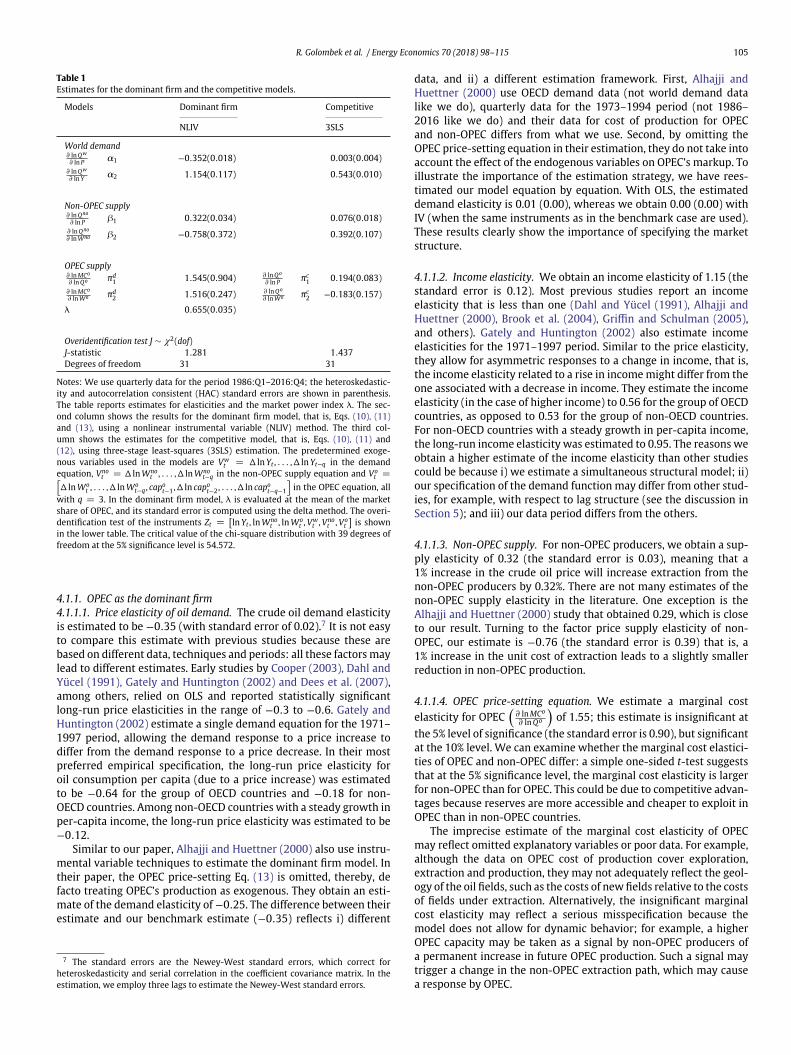
The second column in Table 1 shows our estimates for the domi-nant firm model — Eqs. (10), (11) and (13) — using the NLIV method.The third column in Table 1 shows the estimates from the compet-itive model — Eqs. (10), (11) and (12) — using 3SLS. We use thesame instruments and dummy variables as in the estimation of thedominant firm model.
Table 1 also presents an overidentification test for the instru-ments Zt, see Eq. (15), for the dominant firm model. To test for thevalidity of the instruments, that is, the exogeneity of these variables,we use the Sargan-Hansen J-statistic, which equals the value of theGMM objective function evaluated at the estimated parameters. Wefind that the value of the J-statistic is 1.28. The critical value of thechi-square distribution with 31 degrees of freedom is 29.34 at the5% significance level. Hence, we cannot reject the null hypothesisthat the instruments are exogenous to our system of simultaneousequations.
R. Golombek et al. / Energy Economics 70 (2018) 98–115 105
Table 1Estimates for the dominant firm and the competitive models.
Models Dominant firm Competitive
NLIV 3SLS
World demand∂ ln Qw
∂ ln P a1 −0.352(0.018) 0.003(0.004)∂ ln Qw
∂ ln Y a2 1.154(0.117) 0.543(0.010)
Non-OPEC supply∂ ln Qno
∂ ln P b1 0.322(0.034) 0.076(0.018)∂ ln Qno
∂ ln Wno b2 −0.758(0.372) 0.392(0.107)
OPEC supply∂ ln MCo
∂ ln Qo pd1 1.545(0.904) ∂ ln Qo
∂ ln P pc1 0.194(0.083)
∂ ln MCo
∂ ln Wo pd2 1.516(0.247) ∂ ln Qo
∂ ln Wo pc2 −0.183(0.157)
k 0.655(0.035)
Overidentification test J ∼ w2(dof)J-statistic 1.281 1.437Degrees of freedom 31 31
Notes: We use quarterly data for the period 1986:Q1–2016:Q4; the heteroskedastic-ity and autocorrelation consistent (HAC) standard errors are shown in parenthesis.The table reports estimates for elasticities and the market power index k. The sec-ond column shows the results for the dominant firm model, that is, Eqs. (10), (11)and (13), using a nonlinear instrumental variable (NLIV) method. The third col-umn shows the estimates for the competitive model, that is, Eqs. (10), (11) and(12), using three-stage least-squares (3SLS) estimation. The predetermined exoge-nous variables used in the models are Vw
t = D ln Yt , . . . ,D ln Yt−q in the demandequation, Vno
t = D ln Wnot , . . . ,D ln Wno
t−q in the non-OPEC supply equation and Vot =[
D ln Wot , . . . ,D ln Wo
t−q , capot−1,D ln capo
t−2, . . . ,D ln capot−q−1
]in the OPEC equation, all
with q = 3. In the dominant firm model, k is evaluated at the mean of the marketshare of OPEC, and its standard error is computed using the delta method. The overi-dentification test of the instruments Zt =
[ln Yt , ln Wno
t , ln Wot , Vw
t , Vnot , Vo
t
]is shown
in the lower table. The critical value of the chi-square distribution with 39 degrees offreedom at the 5% significance level is 54.572.
4.1.1. OPEC as the dominant firm4.1.1.1. Price elasticity of oil demand. The crude oil demand elasticityis estimated to be −0.35 (with standard error of 0.02).7 It is not easyto compare this estimate with previous studies because these arebased on different data, techniques and periods: all these factors maylead to different estimates. Early studies by Cooper (2003), Dahl andYücel (1991), Gately and Huntington (2002) and Dees et al. (2007),among others, relied on OLS and reported statistically significantlong-run price elasticities in the range of −0.3 to −0.6. Gately andHuntington (2002) estimate a single demand equation for the 1971–1997 period, allowing the demand response to a price increase todiffer from the demand response to a price decrease. In their mostpreferred empirical specification, the long-run price elasticity foroil consumption per capita (due to a price increase) was estimatedto be −0.64 for the group of OECD countries and −0.18 for non-OECD countries. Among non-OECD countries with a steady growth inper-capita income, the long-run price elasticity was estimated to be−0.12.
Similar to our paper, Alhajji and Huettner (2000) also use instru-mental variable techniques to estimate the dominant firm model. Intheir paper, the OPEC price-setting Eq. (13) is omitted, thereby, defacto treating OPEC’s production as exogenous. They obtain an esti-mate of the demand elasticity of −0.25. The difference between theirestimate and our benchmark estimate (−0.35) reflects i) different
7 The standard errors are the Newey-West standard errors, which correct forheteroskedasticity and serial correlation in the coefficient covariance matrix. In theestimation, we employ three lags to estimate the Newey-West standard errors.
data, and ii) a different estimation framework. First, Alhajji andHuettner (2000) use OECD demand data (not world demand datalike we do), quarterly data for the 1973–1994 period (not 1986–2016 like we do) and their data for cost of production for OPECand non-OPEC differs from what we use. Second, by omitting theOPEC price-setting equation in their estimation, they do not take intoaccount the effect of the endogenous variables on OPEC’s markup. Toillustrate the importance of the estimation strategy, we have rees-timated our model equation by equation. With OLS, the estimateddemand elasticity is 0.01 (0.00), whereas we obtain 0.00 (0.00) withIV (when the same instruments as in the benchmark case are used).These results clearly show the importance of specifying the marketstructure.
4.1.1.2. Income elasticity. We obtain an income elasticity of 1.15 (thestandard error is 0.12). Most previous studies report an incomeelasticity that is less than one (Dahl and Yücel (1991), Alhajji andHuettner (2000), Brook et al. (2004), Griffin and Schulman (2005),and others). Gately and Huntington (2002) also estimate incomeelasticities for the 1971–1997 period. Similar to the price elasticity,they allow for asymmetric responses to a change in income, that is,the income elasticity related to a rise in income might differ from theone associated with a decrease in income. They estimate the incomeelasticity (in the case of higher income) to 0.56 for the group of OECDcountries, as opposed to 0.53 for the group of non-OECD countries.For non-OECD countries with a steady growth in per-capita income,the long-run income elasticity was estimated to 0.95. The reasons weobtain a higher estimate of the income elasticity than other studiescould be because i) we estimate a simultaneous structural model; ii)our specification of the demand function may differ from other stud-ies, for example, with respect to lag structure (see the discussion inSection 5); and iii) our data period differs from the others.
4.1.1.3. Non-OPEC supply. For non-OPEC producers, we obtain a sup-ply elasticity of 0.32 (the standard error is 0.03), meaning that a1% increase in the crude oil price will increase extraction from thenon-OPEC producers by 0.32%. There are not many estimates of thenon-OPEC supply elasticity in the literature. One exception is theAlhajji and Huettner (2000) study that obtained 0.29, which is closeto our result. Turning to the factor price supply elasticity of non-OPEC, our estimate is −0.76 (the standard error is 0.39) that is, a1% increase in the unit cost of extraction leads to a slightly smallerreduction in non-OPEC production.
4.1.1.4. OPEC price-setting equation. We estimate a marginal costelasticity for OPEC
(∂ ln MCo
∂ ln Qo
)of 1.55; this estimate is insignificant at
the 5% level of significance (the standard error is 0.90), but significantat the 10% level. We can examine whether the marginal cost elastici-ties of OPEC and non-OPEC differ: a simple one-sided t-test suggeststhat at the 5% significance level, the marginal cost elasticity is largerfor non-OPEC than for OPEC. This could be due to competitive advan-tages because reserves are more accessible and cheaper to exploit inOPEC than in non-OPEC countries.
The imprecise estimate of the marginal cost elasticity of OPECmay reflect omitted explanatory variables or poor data. For example,although the data on OPEC cost of production cover exploration,extraction and production, they may not adequately reflect the geol-ogy of the oil fields, such as the costs of new fields relative to the costsof fields under extraction. Alternatively, the insignificant marginalcost elasticity may reflect a serious misspecification because themodel does not allow for dynamic behavior; for example, a higherOPEC capacity may be taken as a signal by non-OPEC producers ofa permanent increase in future OPEC production. Such a signal maytrigger a change in the non-OPEC extraction path, which may causea response by OPEC.
106 R. Golombek et al. / Energy Economics 70 (2018) 98–115
The OPEC factor price elasticity(
∂ ln MCo
∂ ln Wo
)is estimated to 1.52 (the
standard error is 0.25). If OPEC production increases, then, ceterisparibus, the market price will fall, which would lower non-OPECproduction, thereby, modifying the initial price reduction. We callthis the equilibrium elasticity of OPEC production
(∂ ln P∂ ln Qo
), and it
is straightforward to identify it in our framework: our estimate is−0.79 (the standard error is 0.05).8 The estimate of the market powerindex k is 0.66, which is clearly above zero. Moreover, the marketpower index estimate is sharply estimated — its standard error isonly 0.04.9 These results suggest that OPEC exerts market power; wereturn to this issue in Section 4.3.
Finally, using our estimated parameters, we find that OPEC’smarkup, see Eq. (7), varies between 2.3 and 8.1 with a mean of 5.3,that is, far above one.10
4.1.2. OPEC as a competitive supplierWe now turn to the estimation of the competitive model: by
comparing the benchmark model with the competitive model, wecan quantify the misspecification bias induced by not accountingfor OPEC taking into consideration that non-OPEC supply dependson OPEC’s level of production, see Eq. (5). The competitive model isestimated using 3SLS.
4.1.2.1. Demand. As seen from the last column in Table 1, the demandelasticity has the wrong sign, but it is small and insignificant; 0.003(0.004) versus −0.35 (0.02) in the benchmark case.11 In the com-petitive model, the estimated income elasticity is 0.54 (0.01), whichis much smaller than the 1.15 estimate in the benchmark case. Thissuggests that not accounting for the non-competitive market struc-ture in the specification of the econometric model leads to biases inthe estimates of the demand and income elasticities.
4.1.2.2. Non-OPEC supply. The supply elasticity of non-OPEC is esti-mated to 0.08 (0.02), which is smaller than in the dominant firmmodel (0.32). The factor price elasticity of non-OPEC is alarming;it has the wrong sign (0.39) and the estimate is significant (thestandard error is 0.11).
4.1.2.3. OPEC supply. When OPEC is assumed to act competitively, itsestimated supply elasticity is 0.19 (0.08), which is small but some-what higher than the supply elasticity of non-OPEC (0.08). The factorprice elasticity of OPEC is insignificantly different from zero.
In summary, the insignificant factor price elasticity of OPEC, aswell as the insignificant demand elasticity, should cast doubt aboutthe empirical relevance of the competitive oil price model. In theremaining part of the paper, we, therefore, focus on the dominantfirm model.
8 Notice that
∂ ln P∂ ln Qo =
14o =
so
a1 − b1 (1 − so).
The equilibrium elasticity is evaluated at the mean of the OPEC market share so . Thestandard error is computed using the delta method. Note that 4o = − 1
0.76 < −1 atequilibrium.
9 The market power index k is evaluated at the mean of the OPEC market share so .The standard error is computed using the delta method.10 Recall that in our estimation, we have imposed that the markup is strictly positive.
Our point estimates clearly meet this restriction.11 The estimate of the demand elasticity in the competitive model can be compared
with Krichene (2006), who estimates a simultaneous equations model for world crudeoil demand and competitive oil supply. Krichene applies the two-stage least-squaremethod to estimate short-run elasticities, and error-correction methods to estimatethe long-run demand elasticity using annual data from 1970 to 2005. He finds thedemand elasticity to vary across countries, ranging from −0.03 to −0.08, whichroughly resembles our result for the competitive model; namely, no price effect ondemand.
4.2. Fit of the dominant firm model
Using the estimated parameters of the dominant firm model,we evaluate the fit of the model using the exogenous variables forthe 1986–2016 period. Then, we perform two counterfactual exper-iments to explore the relative importance of income and cost whenexplaining the long-run trends of price and quantities.
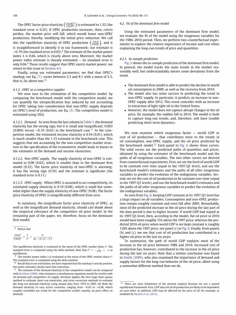
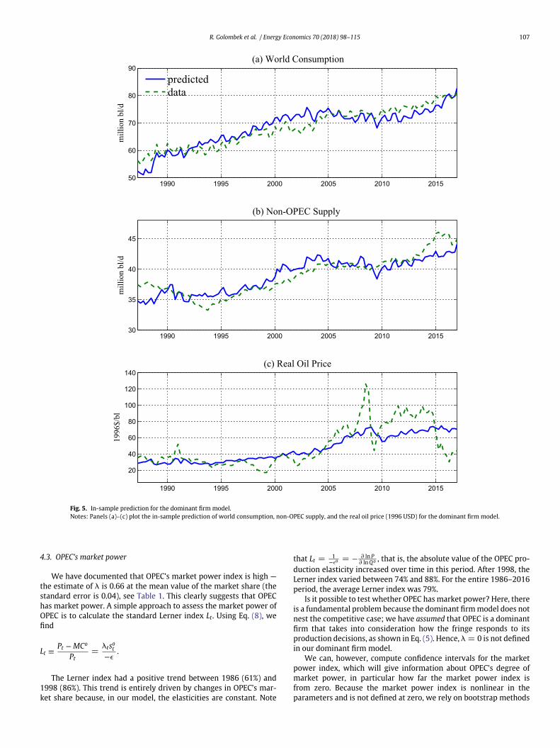
4.2.1. In-sample predictionFig. 5 shows the in-sample prediction of the dominant firm model.
In general, the model tracks the main trends in the market rea-sonably well, but understandably misses some deviations from thetrend.
• The dominant firm model is able to predict the decline in worldoil consumption in 2009, as well as the recovery from 2010.
• The model also has some success in predicting the trend innon-OPEC supply. In particular, it predicts an increase in non-OPEC supply after 2012. This event coincides with an increasein extraction of light tight oil in the United States.
• However, the model does not capture abrupt changes in the oilprice, for example, the sudden fall in 2014. The model is builtto capture long-run trends, and, therefore, will have troublepredicting short-term dynamics.
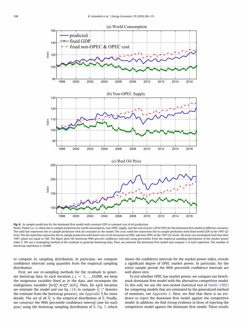
We now examine which exogenous factor — world GDP orcost of oil production — that contributes most to the trends inoil consumption, non-OPEC supply, and the oil price predicted bythe benchmark model.12 Each panel in Fig. 6 shows three curves.The solid curves are the predicted paths of quantities and prices,obtained by using the estimates of the benchmark model and thepaths of all exogenous variables. The two other curves are derivedfrom counterfactual experiments. First, we set the level of world GDPto be constant over time (equal to the 1997:Q1 level), and use thebenchmark model’s estimates and the paths of all other exogenousvariables to predict the evolution of the endogenous variables. Sec-ond, we set the cost of oil production to be constant over time (equalto the 1997:Q1 levels), and use the benchmark model’s estimates andthe paths of all other exogenous variables to predict the evolution ofthe endogenous variables.
As seen from Fig. 6, keeping GDP constant at its 1997:Q1 level hasa large impact on all variables. Consumption and non-OPEC produc-tion remain roughly constant and even fall after 2005. Remarkably,most of the predicted increase in the oil price during the last part ofthe data period is due to higher income: if world GDP had stayed atits 1997:Q1 level, then, according to the model, the oil price in 2016would have been roughly 15% above the 1997 price, whereas the pre-dicted 2016 oil price when world GDP is not kept constant is roughly120% above the 1997 price, see panel (c) in Fig. 6. Finally, from panels(b) and (c), we see that cost of oil production has contributed to ahigher oil price in the last six years.
To summarize, the path of world GDP explains most of theincrease in the oil price between 1986 and 2016. Increased cost ofproduction has, however, contributed to the increase in the oil priceduring the last six years. Note that a similar conclusion was foundin Smith (2009), who also examined the importance of demand andsupply factors for the long-run behavior of the oil price, albeit usinga somewhat different method than we do.
12 There are clear limitations of the present analysis because we use a partialequilibrium framework. First, GDP and cost of oil production are likely to be dependenton each other. In addition, GDP may be affected by the price of oil, for example, asmodeled by Hassler et al. (2012).
R. Golombek et al. / Energy Economics 70 (2018) 98–115 107
1990 1995 2000 2005 2010 201550
60
70
80
90(a) World Consumption
mill
ion
bl/d
predicteddata
1990 1995 2000 2005 2010 201530
35
40
45
(b) Non-OPEC Supply
mill
ion
bl/d
1990 1995 2000 2005 2010 2015
20
40
60
80
100
120
140(c) Real Oil Price
1996
$/bl
Fig. 5. In-sample prediction for the dominant firm model.Notes: Panels (a)–(c) plot the in-sample prediction of world consumption, non-OPEC supply, and the real oil price (1996 USD) for the dominant firm model.
4.3. OPEC’s market power
We have documented that OPEC’s market power index is high —the estimate of k is 0.66 at the mean value of the market share (thestandard error is 0.04), see Table 1. This clearly suggests that OPEChas market power. A simple approach to assess the market power ofOPEC is to calculate the standard Lerner index Lt. Using Eq. (8), wefind
Lt ≡ Pt − MCo
Pt=
ktsot
−4.
The Lerner index had a positive trend between 1986 (61%) and1998 (86%). This trend is entirely driven by changes in OPEC’s mar-ket share because, in our model, the elasticities are constant. Note
that Lt = 1−4o = − ∂ ln P
∂ ln Qo , that is, the absolute value of the OPEC pro-duction elasticity increased over time in this period. After 1998, theLerner index varied between 74% and 88%. For the entire 1986–2016period, the average Lerner index was 79%.
Is it possible to test whether OPEC has market power? Here, thereis a fundamental problem because the dominant firm model does notnest the competitive case; we have assumed that OPEC is a dominantfirm that takes into consideration how the fringe responds to itsproduction decisions, as shown in Eq. (5). Hence, k = 0 is not definedin our dominant firm model.
We can, however, compute confidence intervals for the marketpower index, which will give information about OPEC’s degree ofmarket power, in particular how far the market power index isfrom zero. Because the market power index is nonlinear in theparameters and is not defined at zero, we rely on bootstrap methods
108 R. Golombek et al. / Energy Economics 70 (2018) 98–115
1998 2000 2002 2004 2006 2008 2010 2012 2014 201680
100
120
140
160(a) World Consumption
Inde
x
predictedfixed GDPfixed non-OPEC & OPEC cost
1998 2000 2002 2004 2006 2008 2010 2012 2014 2016
90
100
110
120
130(b) Non-OPEC Supply
Inde
x
1998 2000 2002 2004 2006 2008 2010 2012 2014 2016
100
150
200
250(c) Real Oil Price
Inde
x
Fig. 6. In-sample prediction for the dominant firm model with constant GDP or constant cost of oil production.Notes: Panels (a)–(c) show the in-sample prediction for world consumption, non-OPEC supply, and the real oil price (2010 USD) for the dominant firm model in different scenarios.The solid line represents the in-sample prediction with all covariates in the model. The cross-solid line represents the in-sample prediction with fixed world GDP at the 1997:Q1level. The dot-dash line represents the in-sample prediction with fixed costs of oil extraction in OPEC and non-OPEC at the 1997:Q1 levels. All series are normalized such that their1997 values are equal to 100. The figure plots the bootstrap 99th percent confidence intervals using percentiles from the empirical sampling distribution of the market powerindex k. We use a resampling method of the residuals to generate bootstrap data. Then, we estimate the dominant firm model and compute k in each repetition. The number ofbootstrap repetitions is 10,000.
to compute its sampling distribution. In particular, we computeconfidence intervals using quantiles from the empirical samplingdistribution.
First, we use re-sampling methods for the residuals to gener-ate bootstrap data. In each iteration j, j = 1, . . .,10,000, we keepthe exogenous variables fixed as in the data, and recompute theendogenous variables
[ln Qw
t , ln Qnot , ln Pt
]. Then, for each iteration
we estimate the model and use Eq. (14) to compute k∗j (* denotes
the estimate from the bootstrap process); see Appendix B for moredetails. The set of all k∗
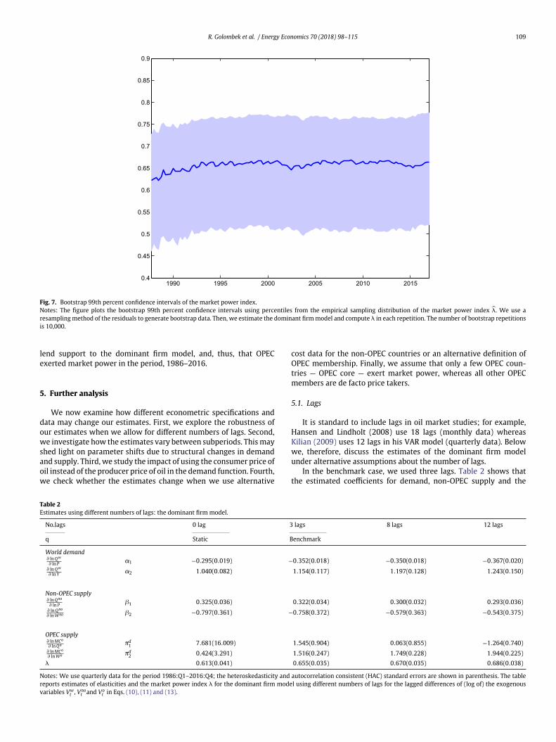
j is the empirical distribution of k. Finally,we construct the 99th percentile confidence interval (one for eachyear) using the bootstrap sampling distribution of k. Fig. 7, which
shows the confidence intervals for the market power index, revealsa significant degree of OPEC market power. In particular, for theentire sample period, the 99th percentile confidence intervals arewell above zero.
To test whether OPEC has market power, we compare our bench-mark dominant firm model with the alternative competitive model.To this end, we use the non-nested statistical test of Smith (1992)for competing models that are estimated by the generalized methodof moments, see Appendix C. Here, we find that there is no evi-dence to reject the dominant firm model against the competitivemodel. In addition, we find strong evidence in favor of rejecting thecompetitive model against the dominant firm model. These results
R. Golombek et al. / Energy Economics 70 (2018) 98–115 109
1990 1995 2000 2005 2010 20150.4
0.45
0.5
0.55
0.6
0.65
0.7
0.75
0.8
0.85
0.9
Fig. 7. Bootstrap 99th percent confidence intervals of the market power index.Notes: The figure plots the bootstrap 99th percent confidence intervals using percentiles from the empirical sampling distribution of the market power index k. We use aresampling method of the residuals to generate bootstrap data. Then, we estimate the dominant firm model and compute k in each repetition. The number of bootstrap repetitionsis 10,000.
lend support to the dominant firm model, and, thus, that OPECexerted market power in the period, 1986–2016.
5. Further analysis
We now examine how different econometric specifications anddata may change our estimates. First, we explore the robustness ofour estimates when we allow for different numbers of lags. Second,we investigate how the estimates vary between subperiods. This mayshed light on parameter shifts due to structural changes in demandand supply. Third, we study the impact of using the consumer price ofoil instead of the producer price of oil in the demand function. Fourth,we check whether the estimates change when we use alternative
cost data for the non-OPEC countries or an alternative definition ofOPEC membership. Finally, we assume that only a few OPEC coun-tries — OPEC core — exert market power, whereas all other OPECmembers are de facto price takers.
5.1. Lags
It is standard to include lags in oil market studies; for example,Hansen and Lindholt (2008) use 18 lags (monthly data) whereasKilian (2009) uses 12 lags in his VAR model (quarterly data). Belowwe, therefore, discuss the estimates of the dominant firm modelunder alternative assumptions about the number of lags.
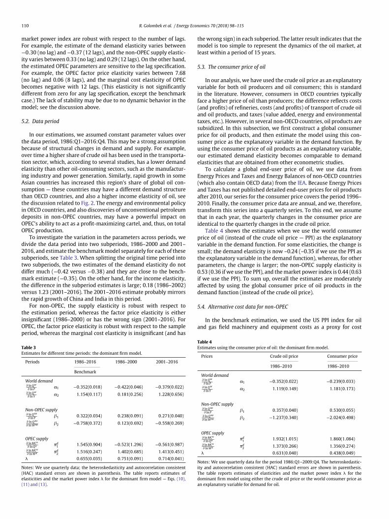
In the benchmark case, we used three lags. Table 2 shows thatthe estimated coefficients for demand, non-OPEC supply and the
Table 2Estimates using different numbers of lags: the dominant firm model.
No.lags 0 lag 3 lags 8 lags 12 lags
q Static Benchmark
World demand∂ ln Qw
∂ ln P a1 −0.295(0.019) −0.352(0.018) −0.350(0.018) −0.367(0.020)∂ ln Qw
∂ ln Y a2 1.040(0.082) 1.154(0.117) 1.197(0.128) 1.243(0.150)
Non-OPEC supply∂ ln Qno
∂ ln P b1 0.325(0.036) 0.322(0.034) 0.300(0.032) 0.293(0.036)∂ ln Qno
∂ ln Wno b2 −0.797(0.361) −0.758(0.372) −0.579(0.363) −0.543(0.375)
OPEC supply∂ ln MCo
∂ ln Qo pd1 7.681(16.009) 1.545(0.904) 0.063(0.855) −1.264(0.740)
∂ ln MCo
∂ ln Wo pd2 0.424(3.291) 1.516(0.247) 1.749(0.228) 1.944(0.225)
k 0.613(0.041) 0.655(0.035) 0.670(0.035) 0.686(0.038)
Notes: We use quarterly data for the period 1986:Q1–2016:Q4; the heteroskedasticity and autocorrelation consistent (HAC) standard errors are shown in parenthesis. The tablereports estimates of elasticities and the market power index k for the dominant firm model using different numbers of lags for the lagged differences of (log of) the exogenousvariables Vw
t , Vnot and Vo
t in Eqs. (10), (11) and (13).
110 R. Golombek et al. / Energy Economics 70 (2018) 98–115
market power index are robust with respect to the number of lags.For example, the estimate of the demand elasticity varies between−0.30 (no lag) and −0.37 (12 lags), and the non-OPEC supply elastic-ity varies between 0.33 (no lag) and 0.29 (12 lags). On the other hand,the estimated OPEC parameters are sensitive to the lag specification.For example, the OPEC factor price elasticity varies between 7.68(no lag) and 0.06 (8 lags), and the marginal cost elasticity of OPECbecomes negative with 12 lags. (This elasticity is not significantlydifferent from zero for any lag specification, except the benchmarkcase.) The lack of stability may be due to no dynamic behavior in themodel; see the discussion above.
5.2. Data period
In our estimations, we assumed constant parameter values overthe data period, 1986:Q1–2016:Q4. This may be a strong assumptionbecause of structural changes in demand and supply. For example,over time a higher share of crude oil has been used in the transporta-tion sector, which, according to several studies, has a lower demandelasticity than other oil-consuming sectors, such as the manufactur-ing industry and power generation. Similarly, rapid growth in someAsian countries has increased this region’s share of global oil con-sumption — these countries may have a different demand structurethan OECD countries, and also a higher income elasticity of oil, seethe discussion related to Fig. 2. The energy and environmental policyin OECD countries, and also discoveries of unconventional petroleumdeposits in non-OPEC countries, may have a powerful impact onOPEC’s ability to act as a profit-maximizing cartel, and, thus, on totalOPEC production.
To investigate the variation in the parameters across periods, wedivide the data period into two subperiods, 1986–2000 and 2001–2016, and estimate the benchmark model separately for each of thesesubperiods, see Table 3. When splitting the original time period intotwo subperiods, the two estimates of the demand elasticity do notdiffer much (−0.42 versus −0.38) and they are close to the bench-mark estimate (−0.35). On the other hand, for the income elasticity,the difference in the subperiod estimates is large; 0.18 (1986–2002)versus 1.23 (2001–2016). The 2001–2016 estimate probably mirrorsthe rapid growth of China and India in this period.
For non-OPEC, the supply elasticity is robust with respect tothe estimation period, whereas the factor price elasticity is eitherinsignificant (1986–2000) or has the wrong sign (2001–2016). ForOPEC, the factor price elasticity is robust with respect to the sampleperiod, whereas the marginal cost elasticity is insignificant (and has
Table 3Estimates for different time periods: the dominant firm model.
Periods 1986–2016 1986–2000 2001–2016
Benchmark
World demand∂ ln Qw
∂ ln P a1 −0.352(0.018) −0.422(0.046) −0.379(0.022)∂ ln Qw
∂ ln Y a2 1.154(0.117) 0.181(0.256) 1.228(0.656)
Non-OPEC supply∂ ln Qno
∂ ln P b1 0.322(0.034) 0.238(0.091) 0.271(0.040)∂ ln Qno
∂ ln Wno b2 −0.758(0.372) 0.123(0.692) −0.558(0.269)
OPEC supply∂ ln MCo
∂ ln Qo pd1 1.545(0.904) −0.523(1.296) −0.561(0.987)
∂ ln MCo
∂ ln Wo pd2 1.516(0.247) 1.402(0.685) 1.413(0.451)
k 0.655(0.035) 0.751(0.091) 0.714(0.041)
Notes: We use quarterly data; the heteroskedasticity and autocorrelation consistent(HAC) standard errors are shown in parenthesis. The table reports estimates ofelasticities and the market power index k for the dominant firm model — Eqs. (10),(11) and (13).
the wrong sign) in each subperiod. The latter result indicates that themodel is too simple to represent the dynamics of the oil market, atleast within a period of 15 years.
5.3. The consumer price of oil
In our analysis, we have used the crude oil price as an explanatoryvariable for both oil producers and oil consumers; this is standardin the literature. However, consumers in OECD countries typicallyface a higher price of oil than producers; the difference reflects costs(and profits) of refineries, costs (and profits) of transport of crude oiland oil products, and taxes (value added, energy and environmentaltaxes, etc.). However, in several non-OECD countries, oil products aresubsidized. In this subsection, we first construct a global consumerprice for oil products, and then estimate the model using this con-sumer price as the explanatory variable in the demand function. Byusing the consumer price of oil products as an explanatory variable,our estimated demand elasticity becomes comparable to demandelasticities that are obtained from other econometric studies.
To calculate a global end-user price of oil, we use data fromEnergy Prices and Taxes and Energy Balances of non-OECD countries(which also contain OECD data) from the IEA. Because Energy Pricesand Taxes has not published detailed end-user prices for oil productsafter 2010, our series for the consumer price covers the period 1996–2010. Finally, the consumer price data are annual, and we, therefore,transform this series into a quarterly series. To this end, we assumethat in each year, the quarterly changes in the consumer price areidentical to the quarterly changes in the crude oil price.
Table 4 shows the estimates when we use the world consumerprice of oil (instead of the crude oil price — PPI) as the explanatoryvariable in the demand function. For some elasticities, the change issmall; the demand elasticity is now –0.24 (–0.35 if we use the PPI asthe explanatory variable in the demand function), whereas, for otherparameters, the change is larger; the non-OPEC supply elasticity is0.53 (0.36 if we use the PPI), and the market power index is 0.44 (0.63if we use the PPI). To sum up, overall the estimates are moderatelyaffected by using the global consumer price of oil products in thedemand function (instead of the crude oil price).
5.4. Alternative cost data for non-OPEC
In the benchmark estimation, we used the US PPI index for oiland gas field machinery and equipment costs as a proxy for cost
Table 4Estimates using the consumer price of oil: the dominant firm model.
Prices Crude oil price Consumer price
1986–2010 1986–2010
World demand∂ ln Qw
∂ ln P a1 −0.352(0.022) −0.239(0.033)∂ ln Qw
∂ ln Y a2 1.119(0.149) 1.181(0.173)
Non-OPEC supply∂ ln Qno
∂ ln P b1 0.357(0.040) 0.530(0.055)∂ ln Qno
∂ ln Wno b2 −1.237(0.340) −2.024(0.498)
OPEC supply∂ ln MCo
∂ ln Qo pd1 1.932(1.015) 1.860(1.084)
∂ ln MCo
∂ ln Wo pd2 1.373(0.266) 1.356(0.274)
k 0.631(0.040) 0.438(0.049)
Notes: We use quarterly data for the period 1986:Q1–2009:Q4. The heteroskedastic-ity and autocorrelation consistent (HAC) standard errors are shown in parenthesis.The table reports estimates of elasticities and the market power index k for thedominant firm model using either the crude oil price or the world consumer price asan explanatory variable for demand for oil.
R. Golombek et al. / Energy Economics 70 (2018) 98–115 111
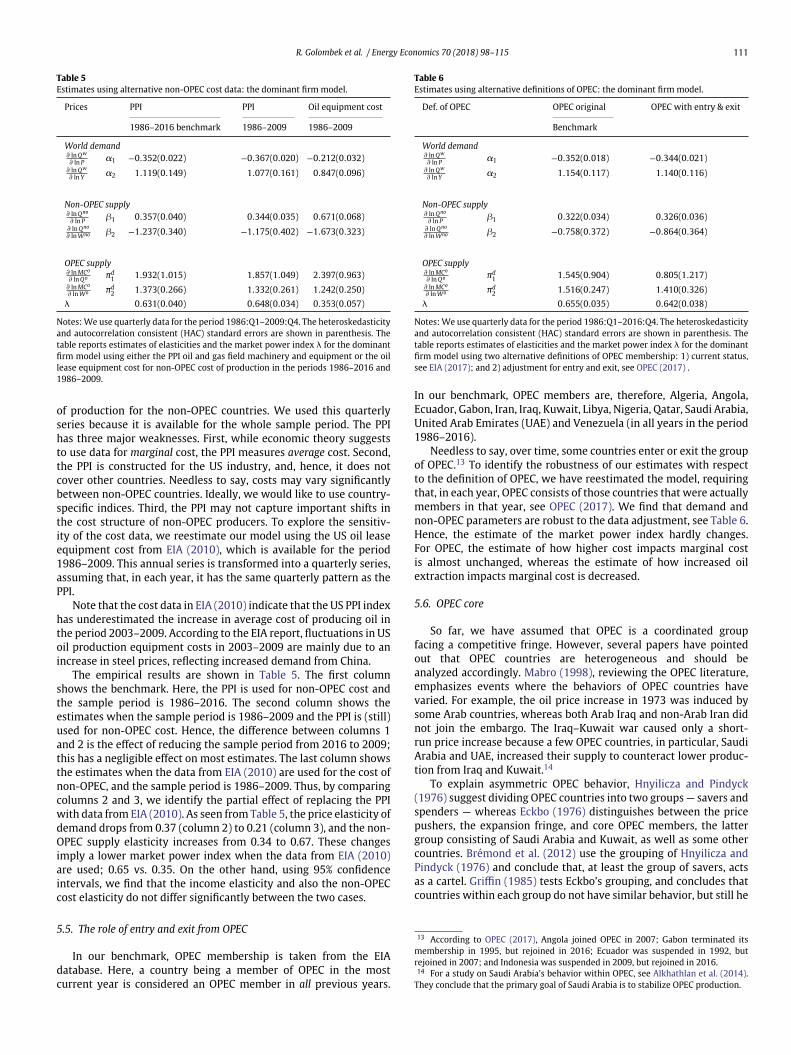
Table 5Estimates using alternative non-OPEC cost data: the dominant firm model.
Prices PPI PPI Oil equipment cost
1986–2016 benchmark 1986–2009 1986–2009
World demand∂ ln Qw
∂ ln P a1 −0.352(0.022) −0.367(0.020) −0.212(0.032)∂ ln Qw
∂ ln Y a2 1.119(0.149) 1.077(0.161) 0.847(0.096)
Non-OPEC supply∂ ln Qno
∂ ln P b1 0.357(0.040) 0.344(0.035) 0.671(0.068)∂ ln Qno
∂ ln Wno b2 −1.237(0.340) −1.175(0.402) −1.673(0.323)
OPEC supply∂ ln MCo
∂ ln Qo pd1 1.932(1.015) 1.857(1.049) 2.397(0.963)
∂ ln MCo
∂ ln Wo pd2 1.373(0.266) 1.332(0.261) 1.242(0.250)
k 0.631(0.040) 0.648(0.034) 0.353(0.057)
Notes: We use quarterly data for the period 1986:Q1–2009:Q4. The heteroskedasticityand autocorrelation consistent (HAC) standard errors are shown in parenthesis. Thetable reports estimates of elasticities and the market power index k for the dominantfirm model using either the PPI oil and gas field machinery and equipment or the oillease equipment cost for non-OPEC cost of production in the periods 1986–2016 and1986–2009.
of production for the non-OPEC countries. We used this quarterlyseries because it is available for the whole sample period. The PPIhas three major weaknesses. First, while economic theory suggeststo use data for marginal cost, the PPI measures average cost. Second,the PPI is constructed for the US industry, and, hence, it does notcover other countries. Needless to say, costs may vary significantlybetween non-OPEC countries. Ideally, we would like to use country-specific indices. Third, the PPI may not capture important shifts inthe cost structure of non-OPEC producers. To explore the sensitiv-ity of the cost data, we reestimate our model using the US oil leaseequipment cost from EIA (2010), which is available for the period1986–2009. This annual series is transformed into a quarterly series,assuming that, in each year, it has the same quarterly pattern as thePPI.
Note that the cost data in EIA (2010) indicate that the US PPI indexhas underestimated the increase in average cost of producing oil inthe period 2003–2009. According to the EIA report, fluctuations in USoil production equipment costs in 2003–2009 are mainly due to anincrease in steel prices, reflecting increased demand from China.
The empirical results are shown in Table 5. The first columnshows the benchmark. Here, the PPI is used for non-OPEC cost andthe sample period is 1986–2016. The second column shows theestimates when the sample period is 1986–2009 and the PPI is (still)used for non-OPEC cost. Hence, the difference between columns 1and 2 is the effect of reducing the sample period from 2016 to 2009;this has a negligible effect on most estimates. The last column showsthe estimates when the data from EIA (2010) are used for the cost ofnon-OPEC, and the sample period is 1986–2009. Thus, by comparingcolumns 2 and 3, we identify the partial effect of replacing the PPIwith data from EIA (2010). As seen from Table 5, the price elasticity ofdemand drops from 0.37 (column 2) to 0.21 (column 3), and the non-OPEC supply elasticity increases from 0.34 to 0.67. These changesimply a lower market power index when the data from EIA (2010)are used; 0.65 vs. 0.35. On the other hand, using 95% confidenceintervals, we find that the income elasticity and also the non-OPECcost elasticity do not differ significantly between the two cases.
5.5. The role of entry and exit from OPEC
In our benchmark, OPEC membership is taken from the EIAdatabase. Here, a country being a member of OPEC in the mostcurrent year is considered an OPEC member in all previous years.
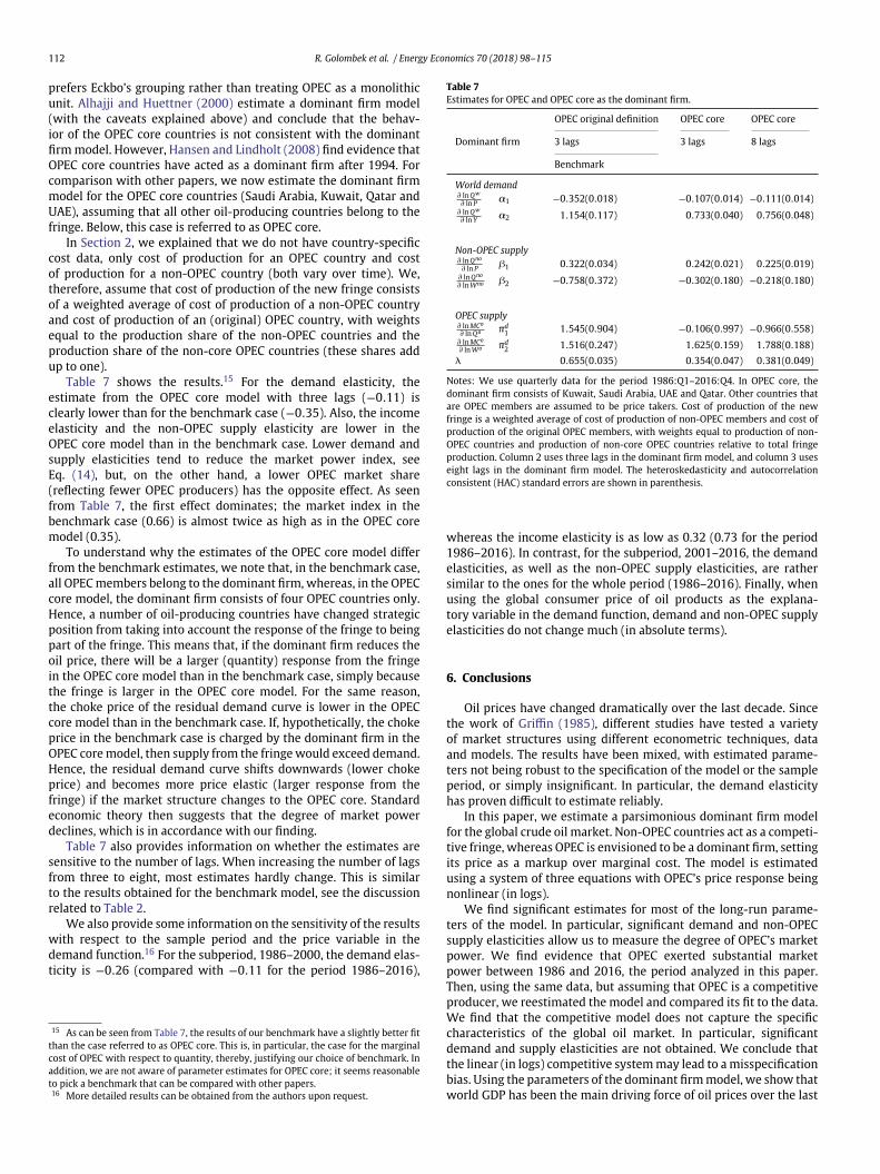
Table 6Estimates using alternative definitions of OPEC: the dominant firm model.
Def. of OPEC OPEC original OPEC with entry & exit
Benchmark
World demand∂ ln Qw
∂ ln P a1 −0.352(0.018) −0.344(0.021)∂ ln Qw
∂ ln Y a2 1.154(0.117) 1.140(0.116)
Non-OPEC supply∂ ln Qno
∂ ln P b1 0.322(0.034) 0.326(0.036)∂ ln Qno
∂ ln Wno b2 −0.758(0.372) −0.864(0.364)
OPEC supply∂ ln MCo
∂ ln Qo pd1 1.545(0.904) 0.805(1.217)
∂ ln MCo
∂ ln Wo pd2 1.516(0.247) 1.410(0.326)
k 0.655(0.035) 0.642(0.038)
Notes: We use quarterly data for the period 1986:Q1–2016:Q4. The heteroskedasticityand autocorrelation consistent (HAC) standard errors are shown in parenthesis. Thetable reports estimates of elasticities and the market power index k for the dominantfirm model using two alternative definitions of OPEC membership: 1) current status,see EIA (2017); and 2) adjustment for entry and exit, see OPEC (2017) .
In our benchmark, OPEC members are, therefore, Algeria, Angola,Ecuador, Gabon, Iran, Iraq, Kuwait, Libya, Nigeria, Qatar, Saudi Arabia,United Arab Emirates (UAE) and Venezuela (in all years in the period1986–2016).
Needless to say, over time, some countries enter or exit the groupof OPEC.13 To identify the robustness of our estimates with respectto the definition of OPEC, we have reestimated the model, requiringthat, in each year, OPEC consists of those countries that were actuallymembers in that year, see OPEC (2017). We find that demand andnon-OPEC parameters are robust to the data adjustment, see Table 6.Hence, the estimate of the market power index hardly changes.For OPEC, the estimate of how higher cost impacts marginal costis almost unchanged, whereas the estimate of how increased oilextraction impacts marginal cost is decreased.
5.6. OPEC core
So far, we have assumed that OPEC is a coordinated groupfacing a competitive fringe. However, several papers have pointedout that OPEC countries are heterogeneous and should beanalyzed accordingly. Mabro (1998), reviewing the OPEC literature,emphasizes events where the behaviors of OPEC countries havevaried. For example, the oil price increase in 1973 was induced bysome Arab countries, whereas both Arab Iraq and non-Arab Iran didnot join the embargo. The Iraq–Kuwait war caused only a short-run price increase because a few OPEC countries, in particular, SaudiArabia and UAE, increased their supply to counteract lower produc-tion from Iraq and Kuwait.14
To explain asymmetric OPEC behavior, Hnyilicza and Pindyck(1976) suggest dividing OPEC countries into two groups — savers andspenders — whereas Eckbo (1976) distinguishes between the pricepushers, the expansion fringe, and core OPEC members, the lattergroup consisting of Saudi Arabia and Kuwait, as well as some othercountries. Brémond et al. (2012) use the grouping of Hnyilicza andPindyck (1976) and conclude that, at least the group of savers, actsas a cartel. Griffin (1985) tests Eckbo’s grouping, and concludes thatcountries within each group do not have similar behavior, but still he
13 According to OPEC (2017), Angola joined OPEC in 2007; Gabon terminated itsmembership in 1995, but rejoined in 2016; Ecuador was suspended in 1992, butrejoined in 2007; and Indonesia was suspended in 2009, but rejoined in 2016.14 For a study on Saudi Arabia’s behavior within OPEC, see Alkhathlan et al. (2014).
They conclude that the primary goal of Saudi Arabia is to stabilize OPEC production.
112 R. Golombek et al. / Energy Economics 70 (2018) 98–115
prefers Eckbo’s grouping rather than treating OPEC as a monolithicunit. Alhajji and Huettner (2000) estimate a dominant firm model(with the caveats explained above) and conclude that the behav-ior of the OPEC core countries is not consistent with the dominantfirm model. However, Hansen and Lindholt (2008) find evidence thatOPEC core countries have acted as a dominant firm after 1994. Forcomparison with other papers, we now estimate the dominant firmmodel for the OPEC core countries (Saudi Arabia, Kuwait, Qatar andUAE), assuming that all other oil-producing countries belong to thefringe. Below, this case is referred to as OPEC core.
In Section 2, we explained that we do not have country-specificcost data, only cost of production for an OPEC country and costof production for a non-OPEC country (both vary over time). We,therefore, assume that cost of production of the new fringe consistsof a weighted average of cost of production of a non-OPEC countryand cost of production of an (original) OPEC country, with weightsequal to the production share of the non-OPEC countries and theproduction share of the non-core OPEC countries (these shares addup to one).
Table 7 shows the results.15 For the demand elasticity, theestimate from the OPEC core model with three lags (−0.11) isclearly lower than for the benchmark case (−0.35). Also, the incomeelasticity and the non-OPEC supply elasticity are lower in theOPEC core model than in the benchmark case. Lower demand andsupply elasticities tend to reduce the market power index, seeEq. (14), but, on the other hand, a lower OPEC market share(reflecting fewer OPEC producers) has the opposite effect. As seenfrom Table 7, the first effect dominates; the market index in thebenchmark case (0.66) is almost twice as high as in the OPEC coremodel (0.35).
To understand why the estimates of the OPEC core model differfrom the benchmark estimates, we note that, in the benchmark case,all OPEC members belong to the dominant firm, whereas, in the OPECcore model, the dominant firm consists of four OPEC countries only.Hence, a number of oil-producing countries have changed strategicposition from taking into account the response of the fringe to beingpart of the fringe. This means that, if the dominant firm reduces theoil price, there will be a larger (quantity) response from the fringein the OPEC core model than in the benchmark case, simply becausethe fringe is larger in the OPEC core model. For the same reason,the choke price of the residual demand curve is lower in the OPECcore model than in the benchmark case. If, hypothetically, the chokeprice in the benchmark case is charged by the dominant firm in theOPEC core model, then supply from the fringe would exceed demand.Hence, the residual demand curve shifts downwards (lower chokeprice) and becomes more price elastic (larger response from thefringe) if the market structure changes to the OPEC core. Standardeconomic theory then suggests that the degree of market powerdeclines, which is in accordance with our finding.
Table 7 also provides information on whether the estimates aresensitive to the number of lags. When increasing the number of lagsfrom three to eight, most estimates hardly change. This is similarto the results obtained for the benchmark model, see the discussionrelated to Table 2.
We also provide some information on the sensitivity of the resultswith respect to the sample period and the price variable in thedemand function.16 For the subperiod, 1986–2000, the demand elas-ticity is −0.26 (compared with −0.11 for the period 1986–2016),
15 As can be seen from Table 7, the results of our benchmark have a slightly better fitthan the case referred to as OPEC core. This is, in particular, the case for the marginalcost of OPEC with respect to quantity, thereby, justifying our choice of benchmark. Inaddition, we are not aware of parameter estimates for OPEC core; it seems reasonableto pick a benchmark that can be compared with other papers.16 More detailed results can be obtained from the authors upon request.
Table 7Estimates for OPEC and OPEC core as the dominant firm.
OPEC original definition OPEC core OPEC core
Dominant firm 3 lags 3 lags 8 lags
Benchmark
World demand∂ ln Qw
∂ ln P a1 −0.352(0.018) −0.107(0.014) −0.111(0.014)∂ ln Qw
∂ ln Y a2 1.154(0.117) 0.733(0.040) 0.756(0.048)
Non-OPEC supply∂ ln Qno
∂ ln P b1 0.322(0.034) 0.242(0.021) 0.225(0.019)∂ ln Qno
∂ ln Wno b2 −0.758(0.372) −0.302(0.180) −0.218(0.180)
OPEC supply∂ ln MCo
∂ ln Qo pd1 1.545(0.904) −0.106(0.997) −0.966(0.558)
∂ ln MCo
∂ ln Wo pd2 1.516(0.247) 1.625(0.159) 1.788(0.188)
k 0.655(0.035) 0.354(0.047) 0.381(0.049)
Notes: We use quarterly data for the period 1986:Q1–2016:Q4. In OPEC core, thedominant firm consists of Kuwait, Saudi Arabia, UAE and Qatar. Other countries thatare OPEC members are assumed to be price takers. Cost of production of the newfringe is a weighted average of cost of production of non-OPEC members and cost ofproduction of the original OPEC members, with weights equal to production of non-OPEC countries and production of non-core OPEC countries relative to total fringeproduction. Column 2 uses three lags in the dominant firm model, and column 3 useseight lags in the dominant firm model. The heteroskedasticity and autocorrelationconsistent (HAC) standard errors are shown in parenthesis.
whereas the income elasticity is as low as 0.32 (0.73 for the period1986–2016). In contrast, for the subperiod, 2001–2016, the demandelasticities, as well as the non-OPEC supply elasticities, are rathersimilar to the ones for the whole period (1986–2016). Finally, whenusing the global consumer price of oil products as the explana-tory variable in the demand function, demand and non-OPEC supplyelasticities do not change much (in absolute terms).
6. Conclusions
Oil prices have changed dramatically over the last decade. Sincethe work of Griffin (1985), different studies have tested a varietyof market structures using different econometric techniques, dataand models. The results have been mixed, with estimated parame-ters not being robust to the specification of the model or the sampleperiod, or simply insignificant. In particular, the demand elasticityhas proven difficult to estimate reliably.
In this paper, we estimate a parsimonious dominant firm modelfor the global crude oil market. Non-OPEC countries act as a competi-tive fringe, whereas OPEC is envisioned to be a dominant firm, settingits price as a markup over marginal cost. The model is estimatedusing a system of three equations with OPEC’s price response beingnonlinear (in logs).
We find significant estimates for most of the long-run parame-ters of the model. In particular, significant demand and non-OPECsupply elasticities allow us to measure the degree of OPEC’s marketpower. We find evidence that OPEC exerted substantial marketpower between 1986 and 2016, the period analyzed in this paper.Then, using the same data, but assuming that OPEC is a competitiveproducer, we reestimated the model and compared its fit to the data.We find that the competitive model does not capture the specificcharacteristics of the global oil market. In particular, significantdemand and supply elasticities are not obtained. We conclude thatthe linear (in logs) competitive system may lead to a misspecificationbias. Using the parameters of the dominant firm model, we show thatworld GDP has been the main driving force of oil prices over the last

R. Golombek et al. / Energy Economics 70 (2018) 98–115 113
three decades. However, rising production costs have contributed toan increase in oil prices after 2004.
The results in this paper suggest some avenues for furtherresearch. First, we used a static model augmented by dynamic factors(lag structure) and lagged OPEC capacity. For the dominant firmmodel, we find that the estimated elasticity of marginal cost ofOPEC with respect to lagged OPEC capacity is significant. Therefore, adynamic approach to understand the role of capacity seems a naturalstep.
One strand of the literature, which builds on Hotelling (1931),singles out resource depletion as the dynamic factor to explain thepath of oil prices. However, attempts to explain long-run prices byfocusing on resource scarcity (see, for example, Lin, 2010, Pindyck,1978; and Jovanovic, 2013) have had limited success, which mayreflect the fact that the size of oil reserves has not changed much overthe last 30 years — new discoveries have compensated for currentextraction (Smith, 2009). An alternative strategy to incorporateresource depletion would be to add dynamics to demand—becauseof financial or inventory speculation17—or dynamics to supply—because of a game between OPEC and non-OPEC where producers(also) choose investment in extraction capacity. This would addpersistency and volatility to prices, thereby, providing a founda-tion for the model to account for the big swings in prices after2000.18 Note, however, that a game between OPEC and non-OPECmay require detailed data on costs of production for each OPECcountry; we have no access to such data.
Acknowledgments
We thank Michele Cavallo, Sigurd Galaasen, Ole Gjølberg, KevinLansing, Carlos Noton, Claudio Raddatz, Eirik Romstad, Knut EinarRosendahl, Gerald Shively, Terje Skjerpen, Kjetil Storesletten andtwo anonymous referees for helpful comments. Earlier versions ofthis paper have been presented at Central Bank of Chile, Universi-dad de Chile — CEA, University of Oslo, Statistics Norway, NorwegianUniversity of Life Sciences — School of Economics and Business, NYU,and the 35th Meeting of the Norwegian Association of Economists.We thank the participants for their comments. We also thank LarsLindholt for sharing his data on OPEC’s production costs, and PaoloGelain for sharing the quarterly world GDP index. The project wasfunded by the Norwegian Research Council under the PETROSAMprogram.
Appendix A. Estimation methods
When OPEC is assumed to be a price taker, the moment conditionfunction g(hc) is defined as
g(hc) =
⎡⎣ Zt (ln Qw
t − Xw′a)Zt (ln Qno
t − Xno′b)Zt (ln Qo
t − Xo′c p
c)
⎤⎦ ,
where Xw, Xno and Xoc are vectors of the right-hand side variables in
Eqs. (10), (11) and (12), respectively. When estimating this system of
17 Kilian and Murphy (2014) develop a structural model for the global crude oil mar-ket and estimate demand elasticities when changes in oil inventory are taken intoaccount. Their results suggest that the 2003–2008 oil price surge was not due tospeculative trading.18 Another potential source of volatility are OPEC announcements about, for
example, changes in production. For studies on how OPEC announcements may haveimpact on oil prices, see, for example, Lin and Tamvakis (2010), Schmidbauer andRösch (2012) and Loutia et al. (2016).
three equations, we use the three-stage least-squares (3SLS) method.The parameter estimates h
care obtained by solving
hc = arg minhc
g(hc)′Wg(hc),
where the weighting matrix W is evaluated at (Z′Z)-1 in the first stepand at (Z′uu′Z)
−1 in the second step, and u =[uw
t , unot , uo
t
]. Because
this model is linear, the system general method of moments (GMM)estimation is equivalent to 3SLS estimation.19
When estimating the dominant firm model, we use the systemnonlinear instrumental variable (NLIV) method with the momentcondition function
g(hd) =
⎡⎢⎣
Zt (ln Qwt − Xw′a)
Zt (ln Qnot − Xno′b)
Zt
(ln Pt − ln m (a1,b1, so
t ) − Xo′d p
d)
⎤⎥⎦ ,
where Xod is the vector of the right-hand side variables in Eq. (13)
except the markup.20 The weighting matrix is evaluated at (Z′Z)-1.21
Appendix B. Construction of confidence intervals
We compute confidence intervals by implementing the followingsteps:
1. Bootstrap data-generating processIn this step, we resample the residuals to generate boot-strap data, that is, we hold the exogenous variables fixed,
but make the endogenous variables[ln Qw
t , ln Qnot , ln Pt
]equal
to the expected values[ln Qw
t , ln Qnot , ln Pt
]plus a resampled
residual u∗j =
[uw∗
tj , uno∗tj , uo∗
tj
]. For the jth repetition, we use
the empirical distribution of the predicted errors (Fox, 2008;MacKinnon et al., 2009):
[ln Qw∗
t , ln Qno∗t , ln P∗
t]
=[ln Qw
t , ln Qnot , ln Pt
]+ u∗
j , u∗j ∼ EDF ( ut)
(* denotes bootstrap data). When we use this method, werely on the regression model to obtain the correct conditionalexpectation, but we do not use the empirical distribution of
19 We have
hc3SLS =
{X′
[Y−1 ⊗ Z(Z′Z)
−1Z′]
X}−1 {
X′[Y−1 ⊗ Z(Z′Z)
−1Z′]
Q}
,
where X =diag([Xw , Xno , Xo]) and Q =[ln Qw
t , ln Qnot , ln Qo
t
]. Further, Y = u′u
N is thecovariance matrix of the residuals from 2SLS where N is the number of observations.The variance matrix can be obtained from
cov(hc
3SLS
)=
{X′
[Y−1 ⊗ Z(Z′Z)
−1Z′]
X}−1
.
20 Although both the markup and the marginal cost of OPEC are functions of OPECsupply, this should not cause a multicollinearity problem because, by using a momentcondition-based method to estimate the model (GMM), we handle the endogeneity ofOPEC supply adequately.21 The variance of this estimator is given by
cov(hd
)=
1N
(G′WG
) (G′WSWG
) (G′WG
)
where G =∂g(hd)
∂hd and S = 1N
∑Ziuiu′
iZi .
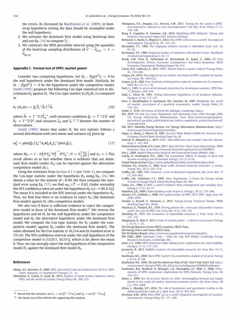
114 R. Golombek et al. / Energy Economics 70 (2018) 98–115
the errors. As discussed by MacKinnon et al. (2009), in boot-strap hypothesis testing the data should be resampled underthe null hypothesis.
2. We estimate the dominant firm model using bootstrap dataand use Eq. (14) to compute k∗
j .3. We construct the 99th percentile interval using the quantiles
of the bootstrap sampling distribution of k∗ : k∗0.5% < k <
k∗99.5%.
Appendix C. Formal test of OPEC market power
Consider two competing hypotheses. Let Hd : E[g(h d)] = 0 bethe null hypothesis under the dominant firm model. Similarly, letHc : E[g(hc)] = 0 be the hypothesis under the competitive model.Smith (1992) proposes the following Cox-type statistical test to dis-criminate Hd against Hc. The Cox-type statistic bT(Hd|Hc) is computedas
bT (Hd|Hc) = g′T S
−1c AT T
12 hT (16)
where AT = T−1Z′ZS−1d , with moment conditions gT = T−1Z′uc and
hT = T−1Z′ud, and variances Sd and Sc.22 T denotes the number ofobservations.
Smith (1992) shows that under Hc the test statistic follows anormal distribution with zero mean and variance y2
d given by
y2d = plim[gT ]′S−1
c AdM′DA′
dS−1c plim [gT ] , (17)
where MD = I − H(
H′S−1d H
)−1H′S−1
d , H = E[
∂hT∂hd
]and Ad = I. This
result allows us to test whether there is evidence that our domi-nant firm model (under Hd) can be rejected against the alternativecompetitive model (Hc).
Using the estimates from Section 4.1.1 (see Table 1), we computethe Cox-type statistic under the hypothesis Hd using Eq. (16). Weobtain a value for the statistic of −0.69. We then compute the stan-dard error using Eq. (17); we find yd/
√T = 0.62. Under normality
the 95% confidence interval under the hypothesis Hd is [−1.90, 0.52].The mean 0 is included in the 95% interval under the hypothesis Hd.Thus, we find that there is no evidence to reject Hd (the dominantfirm model) against Hc (the competitive model).
We also test if there is sufficient evidence to reject the compet-itive model in favor of the dominant firm model.23 We reverse thehypotheses and let Hc be the null hypothesis under the competitivemodel and Hd the alternative hypothesis under the dominant firmmodel. We compute the Cox-type statistic for Hc (under the com-petitive model) against Hd (under the dominant firm model). Thevalue obtained for the Cox statistic is 16,214 and its standard error is151.65. The 95% confidence interval under the null hypothesis of thecompetitive model is [15,917, 16,511], which is far above the mean0. Thus, we can strongly reject the null hypothesis of the competitivemodel Hc against the dominant firm model Hd.
References
Alhajji, A.F., Huettner, D., 2000. OPEC and world crude oil markets from 1973 to 1994:cartel, oligopoly, or competitive? Energy J. 21, 31.
Alkhathlan, K., Gately, D., Javid, M., 2014. Analysis of Saudi Arabia’s behavior withinOPEC and the world oil market. Energy Policy 64, 209–225.
22 Recall that the variances are Sc = var(
T− 12 Z′uc
)and Sd = var
(T− 1
2 Z′ud
).
23 We thank one of the referees for suggesting this analysis.
Almoguera, P.A., Douglas, C.C., Herrera, A.M., 2011. Testing for the cartel in OPEC:noncooperative collusion or just noncooperative? Oxf. Rev. Econ. Policy 27 (1),144–168.
Boug, P., Cappelen, Å., Swensen, A.R., 2016. Modelling OPEC Behavior. Theory andEvidence. Discussion Papers 843. Statistics Norway.
Brémond, V., Hache, E., Mignon, V., 2012. Does OPEC still exist as a cartel?. An empiricalinvestigation. Energy Econ. 34, 125–131.
Bresnahan, T.F., 1982. The oligopoly solution concept is identified. Econ. Lett. 10,87–92.
Bresnahan, T.F., 1989. Empirical Studies of Industries with Market Power. Handbookof Industrial Organization 2, Ch. 17.
Brook, A.M., Price, R., Sutherland, D., Westerlund, N., André, C., 2004. Oil PriceDevelopments: Drivers, Economic Consequences and Policy Responses. OECDEconomics Department Working Papers No. 412.
Cairns, R.D., Calfucura, E., 2012. OPEC: Market failure or power failure? Energy Policy50, 570–580.
Colgan, J.D., 2014. The emperor has no clothes: the limits of OPEC in global oil market.Int. Organ. 68, 599–632.
Cooper, J.C.B., 2003. Price elasticity of demand for crude oil: estimates for 23 countries.OPEC Rev. 27 (1), 1–8.
Dahl, C., 1993. A survey of oil demand elasticities for developing countries. OPEC Rev.17 (Winter), 399–419.
Dahl, C., Yücel, M., 1991. Testing alternative hypotheses of oil producer behavior.Energy J. 12 (4), 117–137.
Dees, S., Karadeloglou, P., Kaufmann, R.K., Sanchez, M., 2007. Modelling the worldoil market: assessment of a quarterly econometric model. Energy Policy 35,179–191.
Eckbo, P., 1976. The Future of World Oil. Ballinger, Cambridge (Mass).EIA, 2010. Oil and Gas Lease Equipment and Operating Costs 1994 through 2009.
U.S. Energy Information Administration. from https://www.eia.gov/pub/oil_gas/natural_gas/data_publications/cost_indices_equipment_production/current/coststudy.html.
EIA, 2017. Monthly Energy Review, U.S. Energy Information Administration. http://www.eia.gov/totalenergy/data/monthly/.
Fagan, G., Henry, J., Mestre, R., 2001. An Area-Wide Model (AWM) for the Euro Area.European Central Bank Working Paper No. 42.
Fattouh, B., Mahadeva, L., 2013. OPEC: what difference has it made? Ann. Rev. Resour.Econ. 5, 427–443.
Federal Reserve Bank of St. Louis, 2017. Spot Oil Price: West Texas Intermediate, FREDEconomic Data. from http://research.stlouisfed.org/fred2/series/OILPRICE.
Fox, J., 2008. Applied Regression Analysis and Generalized Linear Models. Sage.Gately, D., Huntington, H.G., 2002. The asymmetric effects of changes in price and
income on energy and oil demand. Energy J. 23 (1), 9–55.Global Financial Data https://www.globalfinancialdata.com/About/about.html.Graham, D.J., Glaister, S., 2004. Road traffic demand elasticity estimates: a review.
Transp. Rev. 24 (3), 261–274.Griffin, J.M., 1985. OPEC behavior: a test of alternative hypothesis. Am. Econ. Rev. 75
(5), 954–962.Griffin, J.M., Schulman, C.T., 2005. Price Asymmetry: A Proxy for Energy Saving
Technical Change? Bush School Working Paper No. 405.Gulen, S.G., 1996. Is OPEC a cartel? Evidence from cointegration and causality tests.
Energy J. 17 (2), 43–57.Hamilton, J.D., 2009. Understanding crude oil prices. Energy J. 30 (2), 179–206.Hansen, P.V., Lindholt, L., 2008. The market power of OPEC 1973-2001. Appl. Econ. 40,
2939–2959.Hassler, J., Krusell, P., Olovsson, C., 2012. Energy-Saving Technical Change. NBER
Working Paper No. 18456.Hnyilicza, E., Pindyck, R.S., 1976. Pricing policies for a two-part exhaustible resource
cartel: the case of OPEC. Eur. Econ. Rev. 8 (2), 136–154.Hotelling, H., 1931. The economics of exhaustible resources. J. Polit. Econ. 39 (2),
137–175.Huppmann, D., Holz, F., 2012. Crude oil market power — a shift in recent years? Energy
J. 33 (4), 1–22.IEA Energy Balances of non-OECD countries, OECD. Paris.IEA Energy Prices and Taxes, OECD. Paris.IEA Oil Market Report, https://www.iea.org/oilmarketreport/omrpublic/.IHS CERA, 2000. Upstream Costs — Why the Gap Will Widen. Cambridge Energy
Research Associates, Cambridge, MA.Jones, C.T., 1990. OPEC behaviour under falling prices: implications for cartel stability.
Energy J. 11 (3), 117–129.Jovanovic, B., 2013. Bubbles in prices of exhaustible resources. Int. Econ. Rev. 54 (1),
1–34.Kaufmann, R.K., 2004. Does OPEC matter? An econometric analysis of oil price. Energy
J. 25 (4), 67–90.Kaufmann, R.K., 2005. Oil and the American Way of Life: Don’T Ask, Don’t Tell. http://
vmsstreamer1.fnal.gov/VMS_Site_03/Lectures/Colloquium/050601Kaufmann/.Kaufmann, R.K., Bradford, A., Belanger, L.H., Mclaughlin, J.P., Miki, Y., 2008. Deter-
minants of OPEC production: implications for OPEC behavior. Energy Econ. 30,333–351.
Kilian, L., 2009. Not all oil price shocks are alike: disentangling demand and supplyshocks in the crude oil market. American economic review. Am. Econ. Assoc. 99(3), 1053–1069.
Kilian, L., Murphy, D.P., 2014. The role of inventories and speculative trading in theglobal market for crude oil. J. Appl. Econ. 29 (3), 454–478.
Kisswani, K.M., 2016. Does OPEC act as a cartel? Empirical investigation of coordina-tion behavior. Energy Policy 97, 171–180.
R. Golombek et al. / Energy Economics 70 (2018) 98–115 115
Krichene, N., 2002. World crude oil and natural gas: a demand and supply model.Energy Econ. 24, 557–576.
Krichene, N., 2006. World Crude Oil Market: Monetary Policy and the Recent OilShock.IMF Working Paper No. 62.
Lin, C.-Y.C., 2010. An Empirical Dynamic Model of OPEC and Non-OPEC. Workingpaper, University of California at Davis.
Lin, C.Y.C., 2011. Estimating supply and demand in the world oil market. J. Energy Dev.34 (1/2), 1–32.
Lin, S.X., Tamvakis, M., 2010. OPEC announcements and their effects on crude oilprices. Energy Policy 38, 1010–1016.
Loutia, A., Mellios, C., Andriosopoulos, K., 2016. Do OPEC announcements influence oilprices? Energy Policy 90, 262–272.
Mabro, R., 1998. OPEC behaviour 1960–1998: a review of the literature. J. Energy Lit.IV.1, 3–27.
MacKinnon, J.G., 2009. Bootstrap hypothesis testing. In: Belsley, D.A., Kontoghiorghes,E.J. (Eds.), Handbook of Computational Econometrics. John Wiley & Sons Ltd.,Chichester, UK. https://doi.org/10.1002/9780470748916.ch6.
Okullo, S.J., Reynès, F., 2016. Imperfect cartelization in OPEC. Energy Econ. 60,333–344.
OPEC, 2017. Brief History. Organization of the Petroleum Exporting Countries. fromhttp://www.opec.org/opec_web/en/about_us/24.htm.
Pindyck, R.S., 1978. Gains to producers from the cartelization of exhaustible resources.Rev. Econ. Stat. 60 (2), 238–251.
Schmidbauer, H., Rösch, A., 2012. OPEC news announcements: effects on oil priceexpectation and volatility. Energy Econ. 34, 1656–1663.
Smith, J.L., 2005. Inscrutable OPEC? Behavioral Tests of the Cartel Hypothesis. EnergyJ. 26 (1), 51–82.
Smith, J.L., 2009. World oil: market or mayhem? J. Econ. Perspect. 23 (3), 145–164.Smith, R., 1992. Non-nested tests for competing models estimated by generalized
method of moments. Econometrica 60 (4), 973–980.Spilimbergo, A., 2001. Testing the hypothesis of collusive behavior among OPEC
members. Energy Econ. 23, 339–353.Stock, J.H., Watson, M.W., 1993. A simple estimator of cointegrating vectors in higher
order integrated systems. Econometrica 61, 783–820.Suslow, V.Y., 1986. Estimating monopoly behavior with competitive recycling: an
application to Alcoa. RAND J. Econ. 17 (3), 389–403.U.S. Bureau of Labor Statistics, 2017a. Consumer Price Index: All Urban Consumers —
(CPI-U) US City Average (All Items). from http://www.bls.gov/cpi/.U.S. Bureau of Labor Statistics, 2017b. Bureau of Labor Statistics. Oil and Gas Field
Machinery and Equipment Mfg, Producer Price Index Industry Data.from http://data.bls.gov/cgi-bin/surveymost?pc.


