Energy-Sector Fundamentals: Economic Analysis, Projections ... · EnergySector Fundamentals:...
64
CHAPTER 9 EnergySector Fundamentals: Economic Analysis, Projections, and Supply Curves 9.1 EGS in the Energy Sector _ _ _ _ _ _ _ _ _ _ _ _ _ _ _ _ _ _ _ _ _ _ _ _ _ _ _93 9.2 Baseload Electricity Options _ _ _ _ _ _ _ _ _ _ _ _ _ _ _ _ _ _ _ _ _ _ _ _ _95 9.3 Transmission Access _ _ _ _ _ _ _ _ _ _ _ _ _ _ _ _ _ _ _ _ _ _ _ _ _ _ _ _ _95 9.4 Forecasting Baseload Needs _ _ _ _ _ _ _ _ _ _ _ _ _ _ _ _ _ _ _ _ _ _ _ _ _95 9.5 Forecast Demand and Supply Calculations _ _ _ _ _ _ _ _ _ _ _ _ _ _ _ _ _96 9.6 Risk _ _ _ _ _ _ _ _ _ _ _ _ _ _ _ _ _ _ _ _ _ _ _ _ _ _ _ _ _ _ _ _ _ _ _ _ _ _ _97 9.7 Economics and Cost of Energy _ _ _ _ _ _ _ _ _ _ _ _ _ _ _ _ _ _ _ _ _ _ _ _99 9.8 Using Levelized Costs for Comparison _ _ _ _ _ _ _ _ _ _ _ _ _ _ _ _ _ _ _ _99 9.8.1 Fixed costs _ _ _ _ _ _ _ _ _ _ _ _ _ _ _ _ _ _ _ _ _ _ _ _ _ _ _ _ _ _ _ _ _ _ _ _ _910 9.8.2 Variable costs of operation _ _ _ _ _ _ _ _ _ _ _ _ _ _ _ _ _ _ _ _ _ _ _ _ _ _ _ _911 9.8.3 Levelized cost projections _ _ _ _ _ _ _ _ _ _ _ _ _ _ _ _ _ _ _ _ _ _ _ _ _ _ _ _912 9.8.4 Supply and capacity _ _ _ _ _ _ _ _ _ _ _ _ _ _ _ _ _ _ _ _ _ _ _ _ _ _ _ _ _ _ _ _913 9.8.5 The aggregate industry supply curve _ _ _ _ _ _ _ _ _ _ _ _ _ _ _ _ _ _ _ _ _ _914 9.8.6 Geothermal supply characteristics _ _ _ _ _ _ _ _ _ _ _ _ _ _ _ _ _ _ _ _ _ _ _915 9.9 EGS Economic Models _ _ _ _ _ _ _ _ _ _ _ _ _ _ _ _ _ _ _ _ _ _ _ _ _ _ _ _918 9.9.1 GETEM model description _ _ _ _ _ _ _ _ _ _ _ _ _ _ _ _ _ _ _ _ _ _ _ _ _ _ _ _918 9.9.2 Updated MIT EGS model _ _ _ _ _ _ _ _ _ _ _ _ _ _ _ _ _ _ _ _ _ _ _ _ _ _ _ _ _918 9.9.3 Base case and sensitivity _ _ _ _ _ _ _ _ _ _ _ _ _ _ _ _ _ _ _ _ _ _ _ _ _ _ _ _ _918 9.10 Supply Curves and Model Results _ _ _ _ _ _ _ _ _ _ _ _ _ _ _ _ _ _ _ _ _ _924 9.10.1 Supply of EGS power on the edges of existing hydrothermal systems _ _ _ _926 9.10.2 Supply of EGS power from conductive heating _ _ _ _ _ _ _ _ _ _ _ _ _ _ _ _ _927 9.10.3 Effects of learning on supply curves _ _ _ _ _ _ _ _ _ _ _ _ _ _ _ _ _ _ _ _ _ _ _928 9.10.4 Supply curve for EGS _ _ _ _ _ _ _ _ _ _ _ _ _ _ _ _ _ _ _ _ _ _ _ _ _ _ _ _ _ _ _930 9.10.5 EGS well characteristics _ _ _ _ _ _ _ _ _ _ _ _ _ _ _ _ _ _ _ _ _ _ _ _ _ _ _ _ _931 9.11 Learning Curves and Supply Curves _ _ _ _ _ _ _ _ _ _ _ _ _ _ _ _ _ _ _ _ _931 9.12 Forecast Supply of Geothermal Energy _ _ _ _ _ _ _ _ _ _ _ _ _ _ _ _ _ _ _935 9.12.1 The role of technology _ _ _ _ _ _ _ _ _ _ _ _ _ _ _ _ _ _ _ _ _ _ _ _ _ _ _ _ _ _936 91 9.12.2 Variable debt/equity rates vs. fixed charge rates (FCRs) _ _ _ _ _ _ _ _ _ _ _ _939 9.12.3 Deriving cost and supply curves _ _ _ _ _ _ _ _ _ _ _ _ _ _ _ _ _ _ _ _ _ _ _ _ _941 9.13 Conclusions _ _ _ _ _ _ _ _ _ _ _ _ _ _ _ _ _ _ _ _ _ _ _ _ _ _ _ _ _ _ _ _ _ _943 Footnotes _ _ _ _ _ _ _ _ _ _ _ _ _ _ _ _ _ _ _ _ _ _ _ _ _ _ _ _ _ _ _ _ _ _ _ _ _ _944 References _ _ _ _ _ _ _ _ _ _ _ _ _ _ _ _ _ _ _ _ _ _ _ _ _ _ _ _ _ _ _ _ _ _ _ _ _947 Appendices _ _ _ _ _ _ _ _ _ _ _ _ _ _ _ _ _ _ _ _ _ _ _ _ _ _ _ _ _ _ _ _ _ _ _ _ _949
Transcript of Energy-Sector Fundamentals: Economic Analysis, Projections ... · EnergySector Fundamentals:...

C H A P T E R 9
EnergySector Fundamentals: Economic Analysis, Projections, and Supply Curves 9.1 EGS in the Energy Sector _ _ _ _ _ _ _ _ _ _ _ _ _ _ _ _ _ _ _ _ _ _ _ _ _ _ _93
9.2 Baseload Electricity Options _ _ _ _ _ _ _ _ _ _ _ _ _ _ _ _ _ _ _ _ _ _ _ _ _95
9.3 Transmission Access _ _ _ _ _ _ _ _ _ _ _ _ _ _ _ _ _ _ _ _ _ _ _ _ _ _ _ _ _95
9.4 Forecasting Baseload Needs _ _ _ _ _ _ _ _ _ _ _ _ _ _ _ _ _ _ _ _ _ _ _ _ _95
9.5 Forecast Demand and Supply Calculations _ _ _ _ _ _ _ _ _ _ _ _ _ _ _ _ _96
9.6 Risk _ _ _ _ _ _ _ _ _ _ _ _ _ _ _ _ _ _ _ _ _ _ _ _ _ _ _ _ _ _ _ _ _ _ _ _ _ _ _97
9.7 Economics and Cost of Energy _ _ _ _ _ _ _ _ _ _ _ _ _ _ _ _ _ _ _ _ _ _ _ _99
9.8 Using Levelized Costs for Comparison _ _ _ _ _ _ _ _ _ _ _ _ _ _ _ _ _ _ _ _999.8.1 Fixed costs _ _ _ _ _ _ _ _ _ _ _ _ _ _ _ _ _ _ _ _ _ _ _ _ _ _ _ _ _ _ _ _ _ _ _ _ _9109.8.2 Variable costs of operation _ _ _ _ _ _ _ _ _ _ _ _ _ _ _ _ _ _ _ _ _ _ _ _ _ _ _ _9119.8.3 Levelized cost projections _ _ _ _ _ _ _ _ _ _ _ _ _ _ _ _ _ _ _ _ _ _ _ _ _ _ _ _9129.8.4 Supply and capacity _ _ _ _ _ _ _ _ _ _ _ _ _ _ _ _ _ _ _ _ _ _ _ _ _ _ _ _ _ _ _ _9139.8.5 The aggregate industry supply curve _ _ _ _ _ _ _ _ _ _ _ _ _ _ _ _ _ _ _ _ _ _9149.8.6 Geothermal supply characteristics _ _ _ _ _ _ _ _ _ _ _ _ _ _ _ _ _ _ _ _ _ _ _915
9.9 EGS Economic Models _ _ _ _ _ _ _ _ _ _ _ _ _ _ _ _ _ _ _ _ _ _ _ _ _ _ _ _9189.9.1 GETEM model description _ _ _ _ _ _ _ _ _ _ _ _ _ _ _ _ _ _ _ _ _ _ _ _ _ _ _ _9189.9.2 Updated MIT EGS model _ _ _ _ _ _ _ _ _ _ _ _ _ _ _ _ _ _ _ _ _ _ _ _ _ _ _ _ _9189.9.3 Base case and sensitivity _ _ _ _ _ _ _ _ _ _ _ _ _ _ _ _ _ _ _ _ _ _ _ _ _ _ _ _ _918
9.10 Supply Curves and Model Results _ _ _ _ _ _ _ _ _ _ _ _ _ _ _ _ _ _ _ _ _ _9249.10.1 Supply of EGS power on the edges of existing hydrothermal systems _ _ _ _9269.10.2 Supply of EGS power from conductive heating _ _ _ _ _ _ _ _ _ _ _ _ _ _ _ _ _9279.10.3 Effects of learning on supply curves _ _ _ _ _ _ _ _ _ _ _ _ _ _ _ _ _ _ _ _ _ _ _9289.10.4 Supply curve for EGS _ _ _ _ _ _ _ _ _ _ _ _ _ _ _ _ _ _ _ _ _ _ _ _ _ _ _ _ _ _ _9309.10.5 EGS well characteristics _ _ _ _ _ _ _ _ _ _ _ _ _ _ _ _ _ _ _ _ _ _ _ _ _ _ _ _ _931
9.11 Learning Curves and Supply Curves _ _ _ _ _ _ _ _ _ _ _ _ _ _ _ _ _ _ _ _ _931
9.12 Forecast Supply of Geothermal Energy _ _ _ _ _ _ _ _ _ _ _ _ _ _ _ _ _ _ _9359.12.1 The role of technology _ _ _ _ _ _ _ _ _ _ _ _ _ _ _ _ _ _ _ _ _ _ _ _ _ _ _ _ _ _936 91
9.12.2 Variable debt/equity rates vs. fixed charge rates (FCRs) _ _ _ _ _ _ _ _ _ _ _ _9399.12.3 Deriving cost and supply curves _ _ _ _ _ _ _ _ _ _ _ _ _ _ _ _ _ _ _ _ _ _ _ _ _941
9.13 Conclusions _ _ _ _ _ _ _ _ _ _ _ _ _ _ _ _ _ _ _ _ _ _ _ _ _ _ _ _ _ _ _ _ _ _943
Footnotes _ _ _ _ _ _ _ _ _ _ _ _ _ _ _ _ _ _ _ _ _ _ _ _ _ _ _ _ _ _ _ _ _ _ _ _ _ _944
References _ _ _ _ _ _ _ _ _ _ _ _ _ _ _ _ _ _ _ _ _ _ _ _ _ _ _ _ _ _ _ _ _ _ _ _ _947
Appendices _ _ _ _ _ _ _ _ _ _ _ _ _ _ _ _ _ _ _ _ _ _ _ _ _ _ _ _ _ _ _ _ _ _ _ _ _949

Chapter 9 EnergySector Fundamentals: Economic Analysis, Projections, and Supply Curves
9.1 EGS in the Energy Sector Geothermal operations have been in place with varying degrees of complexity and use of technology since the turn of the previous century. These operations occupy a range of technologies from geothermal heat pumps through advanced binary and flash plant facilities that produce electric power. Costs of operation for existing plants are welldocumented (see references) and reflect the conditions of drilling and operation for primarily hydrothermal wells at depths that do not exceed 4 km for typically electric utilities that are commercially operated.
Highgrade hydrothermal systems exist because natural permeability allows naturally present water to circulate to shallow depths. The circulating hot water heats surrounding rock to some distance away from the permeability anomaly, according to the length of time the system has been in existence. These systems rely primarily on convective heating rather than the conductive heating from the resource base. In hydrothermal systems, the thermal energy accessible for recovery is limited to the thermodynamic availability of the fluids in the natural system consisting of the convective cell. Such systems require (1) abnormally high heat flow, (2) significant permeability to compensate for the low thermal conductivity of rock, (3) the presence of significant storage porosity for containing the fluid, and (4) the fluid itself. The exploitation of hydrothermal systems requires the fortuitous collocation of these four conditions.
Enhanced Geothermal Systems (EGS) differ fundamentally from these hydrothermal systems. EGS engineering technology provides means for mining heat from a portion of the universally present stored thermal energy contained in rock at depths of interest, by designing and stimulating a reservoir whose production characteristics would be similar to a commercial hydrothermal system. For highgrade EGS resources, the high heat flow requirement (1) is met, while lower EGS grades are also generally accessible using EGS technology, albeit at higher cost. EGS provides engineering options for satisfying the remaining requirements – (2)(4). Consequently, the number of potential sites suitable for EGS is significantly greater than for hydrothermal. Ultimately, the EGS approach may be universally applicable, assuming continued, longerterm R&D support for advanced exploration, reservoir stimulation and drilling, and technologies.
Electric utilities are defined as either privately owned companies or publicly owned agencies that engage in the supply (including generation, transmission, and/or distribution) of electric power. Nonutilities are privately owned companies that generate power for their own use and/or for sale to utilities and others.
The generating units operated by an electric utility vary by intended use, that is, by the three major types of load requirements the utility must meet, generally categorized as base, intermediate, and 93
peak. A baseload generating unit is normally used to satisfy all or part of the minimum or base demand of the system and, as a consequence, produces electricity essentially at a constant rate and runs continuously. Baseload units are generally the largest of the three types of units, but they cannot be brought online or taken offline quickly. Peakload generating units can be brought online quickly and are used to meet requirements during the periods of greatest load on the system. They are normally smaller plants using gas turbines, and/or combined cycle steam and gas turbines. Intermediateload generating units meet system requirements that are greater than base load but less than peak load. Intermediateload units are used during the transition between baseload and peakload requirements (EIA, 2005; Stoft, 2002).

Chapter 9 EnergySector Fundamentals: Economic Analysis, Projections, and Supply Curves
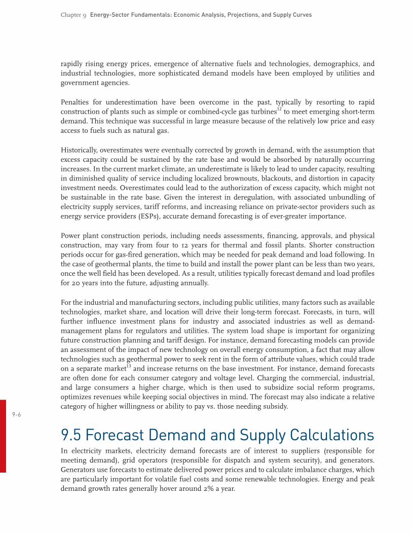
The history of electricity generation in the United States and projections to 2020 are shown in Figure 9.1 for all resources. It is important to note that the projected demand for electricity assumes thatthere are no major policy initiatives to offset current demand growth trends. Even if policies were put in place to reduce demand by improving efficiency in all forms of energy use, a growing U.S. population will eventually lead to some growth in demand that could be met by further development of renewables, including new forms such as environmentally friendly EGS.
A key characteristic of renewable hydrothermal geothermal power is the longterm stability of the resource and characteristic power curve. This power curve is valued by utility or grid operators for baseload conditions where load following or rapidly changing load operations do not need to be met. Geothermal plants run at all times through the year except in the case of repairs or scheduled maintenance.
A baseload power plant is one that provides a steady flow of power regardless of total power demand by the grid.1* Power generation units are designated baseload according to their efficiency and safety at set designed outputs. Baseload power plants do not change production to match power consumption demands. Generally, these plants are massive enough, usually greater than 250 MWe, to provide a significant portion of the power used by a grid in everyday operations with consequent long rampup and rampdown times. Capacity factors are typically in excess of 90%. Fluctuations in power supply demand, the peak power demand, or spikes in customer demand are handled by smaller and more responsive types of power plants.
94
3,500
3,000
2,500
2,000
1,500
1,000
500
1970
1970 2020
4,916
1,392
Electricity demandProjections
Coal
Natural Gas
Nuclear
RenewablesPetroleum
1980 1990 2000Year
Elec
tric
ity
gene
rati
on(1
06M
Wh)
2010 20200
Figure 9.1 U.S. electricity generation by energy source, 19702020 (million megawatthours) (EIA, 2004).
* Numbered footnotes are located before the references at the end of this chapter.

Chapter 9 EnergySector Fundamentals: Economic Analysis, Projections, and Supply Curves
9.2 Baseload Electricity OptionsSteamelectric (thermal) generating units are the typical source of baseload power. A significant fraction of North American baseload power is provided by fossil fuels such as coal, which are burned in a boiler to produce steam. Nuclear plants use nuclear fission as the heat source to make steam. Geothermal or solarthermal energy can also be used to produce steam. The expected thermal efficiency of fossilfueled steamelectric plants is about 33% to 35%. In the case of fossilfired plants, waste heat is emitted from the plant either directly into the atmosphere, through a cooling tower, or into water bodies for cooling where a pump brings the residual water from the condenser back to the boiler. In the case of geothermal power, condensed geofluid is used for cooling water makeup and the residual water is reinjected into the well system.
Because geothermal power plants are usually operated as baseload units, we include a detailed assessment of the state of U.S. electrical supply and demand to illustrate how EGS plants would complement the existing and projected supply system. This discussion is found in Appendix A.9.1.
9.3 Transmission AccessAccess to the electricity grid and, ultimately, the market is a key cost consideration for geothermal projects.9 The necessary power transmission system involves the transportation of large blocks of power over relatively long distances from a central generating station to main substations close to major load centers, or from one central station to another for load sharing.
Highvoltage transmission lines are used because they require less surface area for a given carrying power capacity, and result in less line loss. According to the Energy Information Administration (EIA), in the United States, investorowned utilities (IOUs) own 73% of the transmission lines, federally owned utilities own 13%, and public utilities and cooperative utilities own 14%. Not all utilities own transmission lines (i.e., they are not vertically integrated), and no independent power producers or power marketers own transmission lines. Over the years, these transmission lines have evolved into three major networks (power grids), which include smaller groupings or power pools. The major networks consist of extrahighvoltage connections between individual utilities, designed to permit the transfer of electrical energy from one part of the network to another. These transfers are restricted, on occasion, because of a lack of contractual arrangements or because of inadequate transmission capability.
Power generated from geothermal plants of all kinds is delivered as alternating current (AC) power, 10
which is suitable for dispatch by grid operators or for wheeling to other demand locations. Bulk 95 transmission is also an option when costs of power are low enough, to distant markets via direct
11current (DC) transmission facilities. Distances of more than 1,000 miles combined with a threshold of 1,000 MWe are typically necessary to justify the costs of service obtained by using DC lines.
9.4 Forecasting Baseload NeedsForecasting demand for an electric utility is critical for delivering reliable power, for estimating future costs, and for encouraging new investment. In the past, power system operators relied on straightline extrapolations of historical energy consumption trends. However, given inflation with
Chapter 9 EnergySector Fundamentals: Economic Analysis, Projections, and Supply Curves
rapidly rising energy prices, emergence of alternative fuels and technologies, demographics, and industrial technologies, more sophisticated demand models have been employed by utilities and government agencies.
Penalties for underestimation have been overcome in the past, typically by resorting to rapid construction of plants such as simple or combinedcycle gas turbines12 to meet emerging shortterm demand. This technique was successful in large measure because of the relatively low price and easy access to fuels such as natural gas.
Historically, overestimates were eventually corrected by growth in demand, with the assumption that excess capacity could be sustained by the rate base and would be absorbed by naturally occurring increases. In the current market climate, an underestimate is likely to lead to under capacity, resulting in diminished quality of service including localized brownouts, blackouts, and distortion in capacity investment needs. Overestimates could lead to the authorization of excess capacity, which might not be sustainable in the rate base. Given the interest in deregulation, with associated unbundling of electricity supply services, tariff reforms, and increasing reliance on privatesector providers such as energy service providers (ESPs), accurate demand forecasting is of evergreater importance.
Power plant construction periods, including needs assessments, financing, approvals, and physical construction, may vary from four to 12 years for thermal and fossil plants. Shorter construction periods occur for gasfired generation, which may be needed for peak demand and load following. In the case of geothermal plants, the time to build and install the power plant can be less than two years, once the well field has been developed. As a result, utilities typically forecast demand and load profiles for 20 years into the future, adjusting annually.
For the industrial and manufacturing sectors, including public utilities, many factors such as available technologies, market share, and location will drive their longterm forecast. Forecasts, in turn, will further influence investment plans for industry and associated industries as well as demandmanagement plans for regulators and utilities. The system load shape is important for organizing future construction planning and tariff design. For instance, demand forecasting models can provide an assessment of the impact of new technology on overall energy consumption, a fact that may allow technologies such as geothermal power to seek rent in the form of attribute values, which could trade on a separate market13 and increase returns on the base investment. For instance, demand forecasts are often done for each consumer category and voltage level. Charging the commercial, industrial, and large consumers a higher charge, which is then used to subsidize social reform programs, optimizes revenues while keeping social objectives in mind. The forecast may also indicate a relative category of higher willingness or ability to pay vs. those needing subsidy.
96
9.5 Forecast Demand and Supply Calculations In electricity markets, electricity demand forecasts are of interest to suppliers (responsible for meeting demand), grid operators (responsible for dispatch and system security), and generators. Generators use forecasts to estimate delivered power prices and to calculate imbalance charges, which are particularly important for volatile fuel costs and some renewable technologies. Energy and peak demand growth rates generally hover around 2% a year.
Chapter 9 EnergySector Fundamentals: Economic Analysis, Projections, and Supply Curves
New demand for baseload power is determined by a wide variety of factors including growth in overall demand for power by sector, retirement of existing generation units, operator costs, and cost of transmission access. Competitive access to the grid will always be a function of location, competitive power prices, reliability of delivered power supplies, and the ongoing demand structure of the region into which the power is delivered.
Demand is generally a function of population growth, housing demand, and energy intensity of operations in both the industrial and commercial sectors of the economy. In the case of electricity demand, changes in overall demand generally reflect the ability of individuals or businesses in a particular sector to monitor and adjust activities in response to changes in delivered energy prices. Thus, applications of energysaving or energy efficiency technologies will have an immediate impact on lowering demand, and may reduce the overall slope of the demand for the future. This demand will be driven by growth in population and more reliance on electricintensive appliances, devices, computers, and, eventually, electric or hybrid vehicles.
Baseload power is competitively acquired by system operators, generally in longterm contracts. As a consequence, price for delivered energy does not vary significantly over time, although the price may vary between regions. The growth in energy services reflects an increase in population and economic activity, tempered by improved efficiency of equipment and buildings.
However, the present coincidence of domestic petroleum reserve issues and international politics, the failure to keep up with energy infrastructure requirements, the slow rebirth of the nuclear option due to continued public resistance and nonsupportive regulatory/permitting policies, growing pressure to limit the environmental costs of coal production and utilization, and the pervasive pressure for reduction of CO2 emissions all will work against the traditional ability of technology to match demand growth. As current energy contracts expire and societal/cultural impediments affect expanded use of nuclear and coal, upward price trends for electricity should result over the near to long term.
9.6 RiskThe level of risk for the project must account for all potential sources of risk: technology, scheduling, finances, politics, and exchange rate. The level of risk generally will define whether or not a project can be financed and at what rates of return.
Current hydrothermal projects or future EGS projects will, in the near term, carry considerable risk as viewed in the power generation and financial community. Risk can be expressed in a variety of ways including cost of construction, construction delays, or drilling cost and/or reservoir production 97 uncertainty. In terms of “fuel” supply (i.e., the reliable supply of produced geofluids with specified flow rates and heat content, or enthalpy), a critical variable in geothermal power delivery, risks initially are high but become very low once the resource has been identified and developed to some degree, reflecting the attraction of this as a dependable baseload resource.
Table 9.1 lists the costs and risks associated with the stages of geothermal power development. The risks are qualitative assessments, based on our understanding of the facets of each of the diverse project activities.

Chapter 9 EnergySector Fundamentals: Economic Analysis, Projections, and Supply Curves
Table 9.1 Stages of EGS development: costs and risk
Geologic assessment and permits
Category Duration Cost Risk
Define areas of potential development 12 years Moderate Low
Exclude areas of public protection, high environmental impact, or protected zones
12 years Moderate Low
Determine regional high to lowheat gradient zones 12 years Moderate Low
Correlate with areas of forecast demand growth or baseload retirement
1 year Low Moderate
Determine regional variations in drilling costs, labor costs, grid integration
< 1 year Low Moderate
Determine need for voltage and VARS14 support < 1 year Low Moderate
Determine regulation constraints < 1 year Low Moderate
Determine taxation policies < 1 year Low Moderate
Estimate market or government subsidies < 1 year Low Moderate
Estimate costs 1 year Low Moderate
File for permit and mitigate environmental externalities 3+ years High High
Apply for transmission interconnect < 1 year Moderate High
Acquire permit and begin drilling 1 month Moderate Low
Exploratory drilling
Category Duration Cost Risk
Site improvement 1 month Moderate Moderate
Determine reservoir characteristics (rock type, gradient, stimulation properties, etc.)
6 months High High
Performance/productivity (flow rate, temperature, fluid
quality, etc.) 6 months High High
Apply and test advances in drilling and fracturing technology
6 months High High
98
Achieve cost reductions as function of recent research and
past learning curve 6 months High High
Production drilling and reservoir stimulation
Category Duration Cost Risk
Apply best practices and further develop site 1 year High Moderate
Construct transmission interconnection 2 months Moderate Moderate
Construct power transmission facility 2 months High Moderate
Construct power conversion system 2 years High Low

Chapter 9 EnergySector Fundamentals: Economic Analysis, Projections, and Supply Curves
Table 9.1 continued
Power production and market performance
Category Duration Cost Risk
Bid long based on expected delivery costs Routine and
recurring Low High
Estimate competitive fuel and delivery costs for existing
baseload power
Routine and
recurring Low High
Enter power purchase agreement Infrequent Moderate High
9.7 Economics and Cost of EnergyGeothermal energy – which is transformed into delivered energy (electricity or direct heat) – is an extremely capitalintensive and technologydependent industry. The capital investment may be characterized in three distinct phases:
a) Exploration and drilling of test and production wells b) Construction of power conversion facilities c) Discounted future redrilling and well stimulation.
Previous estimates of capital cost by the California Energy Commission (CEC, 2006), showed that capital reimbursement and interest charges accounted for 65% of the total cost of geothermal power. The remainder covers fuel (water), parasitic pumping loads, labor and access charges, and variable costs. By way of contrast, the capital costs of combinedcycle natural gas plants are estimated to represent only about 22% of the levelized cost of energy produced, with fuel accounting for up to 75% of the delivered cost of energy.
Given the high initial capital cost, most EGS facilities will deliver baseload power to grid operations under a longterm power purchase agreement (typically greater than 10 years) in order to acquire funding for the capital investment. We have assumed that loan life will typically be 30 years, and that the life span of surface capital facilities will be 70 years with incremental improvements or repairs to the installed technology during that period. We assume that the life of the well field will be 30 years with periodic (approximately seven to 10 years) redrilling, fracturing, and hydraulic stimulation during that period. At the end of a 30year cycle, the well complex is assumed to be abandoned, but the surface facilities can service new well complexes through extension of piping and delivery systems with no appreciable loss. Delivered cost of energy is, thus, a function of this stream of capital
99investment and refurbishment, and ongoing operations and delivery costs.
The upshot of this analytical technique is to allow comparison with existing fossil and other renewable technologies such as wind and hydroelectric, where similar capital facility life span can be expected.
9.8 Using Levelized Costs for ComparisonThe delivered cost of electricity is the primary criterion for any electric power generation technology. The levelized cost of energy (or levelized electricity cost, LEC) is the most common approach used for
Chapter 9 EnergySector Fundamentals: Economic Analysis, Projections, and Supply Curves
comparing the cost of power from competing technologies. The levelized cost of energy is found from the present value of the total cost of building and operating a generating plant over its expected economic life. Costs are levelized in real dollars, i.e., adjusted to remove the impact of inflation.
There are two common approaches for calculating the LEC. The first, a simplified approach, calculates a total annualized cost using a fixed charge rate applied to invested capital, adds an annualized operating cost, and divides the sum by the annual electric generation. The second approach uses a full financial cashflow model to perform a similar calculation. The latter approach is usually preferred because it takes into account a wide range of cost parameters that any project must face. As pointed out by the EIA, the cost of power must be competitive with other power generation options after taking into account any special incentives available to the technology. This could include greenpricing production incentives, grants (such as those from the California Energy Commission to improve drilling techniques), subsidies or required purchases through renewable energy portfolio standards, or special tax incentives.
9.8.1 Fixed costs
Any power production facility is subject to a range of fixed and variable costs. Comparing power development opportunities requires like units of measure, typically capitalized costs of fixed assets and the levelized costs of operation.
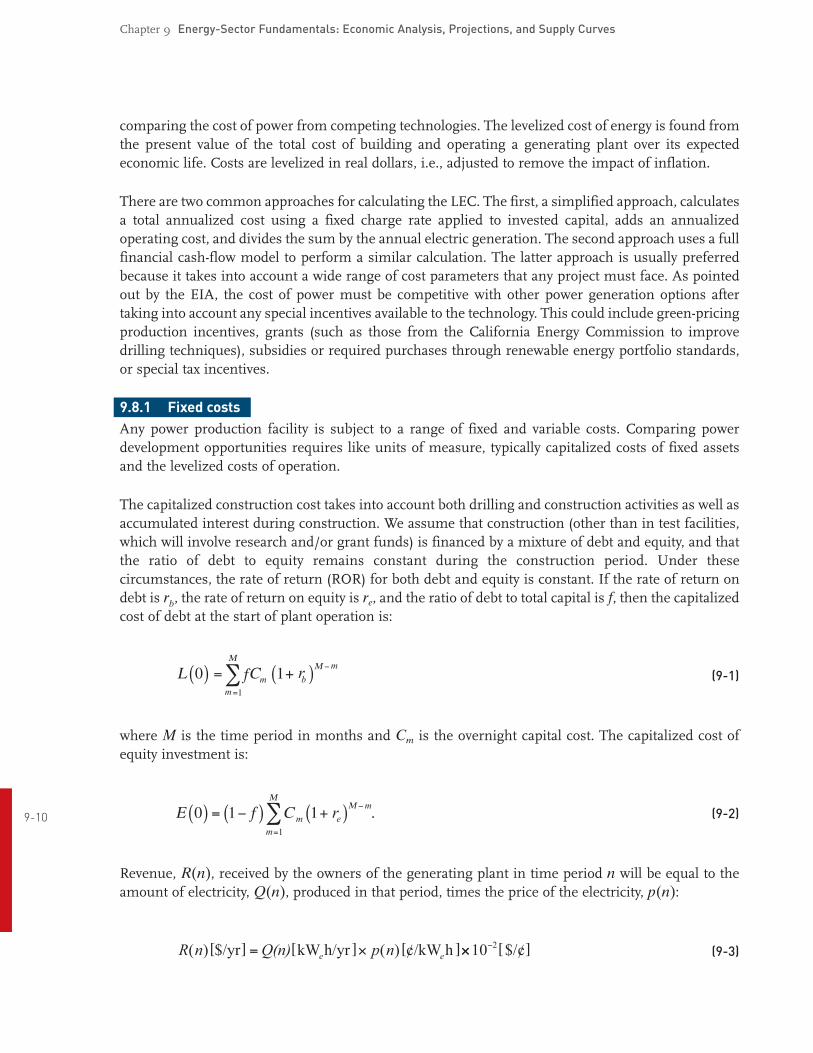
The capitalized construction cost takes into account both drilling and construction activities as well as accumulated interest during construction. We assume that construction (other than in test facilities, which will involve research and/or grant funds) is financed by a mixture of debt and equity, and that the ratio of debt to equity remains constant during the construction period. Under these circumstances, the rate of return (ROR) for both debt and equity is constant. If the rate of return on debt is rb, the rate of return on equity is re, and the ratio of debt to total capital is f, then the capitalized cost of debt at the start of plant operation is:
(91)
where M is the time period in months and Cm is the overnight capital cost. The capitalized cost of equity investment is:
(92)910
Revenue, R(n), received by the owners of the generating plant in time period n will be equal to the amount of electricity, Q(n), produced in that period, times the price of the electricity, p(n):
(93)

Chapter 9 EnergySector Fundamentals: Economic Analysis, Projections, and Supply Curves
where
(94)
We assume K is the rated capacity (in MWe) of the plant15 and CF(n) is the capacity factor of the plant in time period n. The capacity factor will gradually decline over time, but for the assumed period of this analysis, is taken as constant. Thus,
(95)
9.8.2 Variable costs of operation
Costs of operation consist of fuels (water for injection, electricity for parasitic power pumping load), operations and maintenance (excluding the cost of redrilling or stimulation, which are assumed in capital cost calculations), interest and principal repayments, taxes, and depreciation. In addition, shareholder returns on equity, re, are counted when a project is commercial, as opposed to experimental.
(96)
where:
TVc = Total annual variable cost Tx = Tax payment on income and property F = Annual fuel cost
(97)
where:
cfuel(n) = the fuel cost expressed in $/kWh in year n Om = Annual Operations and Maintenance
(98) 911
where:
cO&M(n) = the unit O&M cost expressed in $/kWh. The fixed cost component of O&M is ignored. Dq = combined debt and equity service in equal annual installments over a term of N years.
The term Dq reflects not only market cost but risk (for example, the higher risk of equity versus borrowed capital) when re > rb. This places a relative premium on payments over the project lifetime.
Chapter 9 EnergySector Fundamentals: Economic Analysis, Projections, and Supply Curves
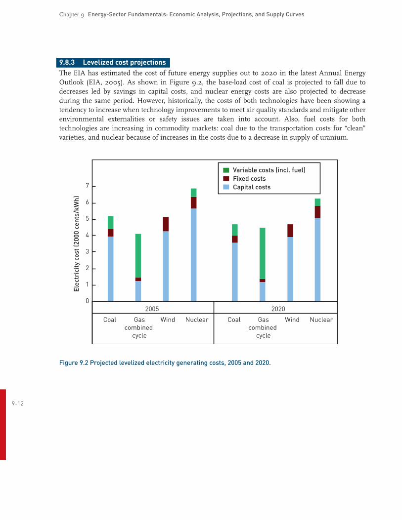
9.8.3 Levelized cost projections
The EIA has estimated the cost of future energy supplies out to 2020 in the latest Annual Energy Outlook (EIA, 2005). As shown in Figure 9.2, the baseload cost of coal is projected to fall due to decreases led by savings in capital costs, and nuclear energy costs are also projected to decrease during the same period. However, historically, the costs of both technologies have been showing a tendency to increase when technology improvements to meet air quality standards and mitigate other environmental externalities or safety issues are taken into account. Also, fuel costs for both technologies are increasing in commodity markets: coal due to the transportation costs for “clean” varieties, and nuclear because of increases in the costs due to a decrease in supply of uranium.
Coal
20050
1
2
3
4
5
6
7
2020
Gascombined
cycle
Gascombined
cycle
Variable costs (incl. fuel)Fixed costsCapital costs
Elec
tric
ity
cost
(200
0ce
nts/
kWh)
Wind Nuclear Coal Wind Nuclear
Figure 9.2 Projected levelized electricity generating costs, 2005 and 2020.
912
Chapter 9 EnergySector Fundamentals: Economic Analysis, Projections, and Supply Curves
9.8.4 Supply and capacity
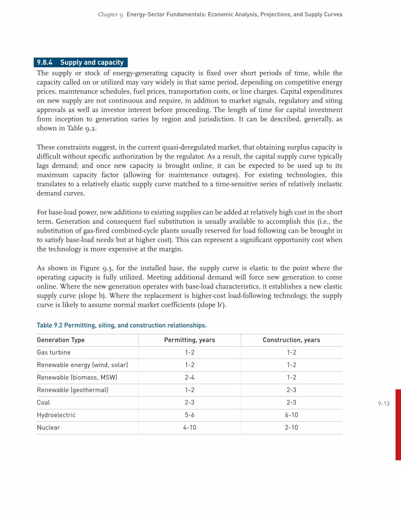
The supply or stock of energygenerating capacity is fixed over short periods of time, while the capacity called on or utilized may vary widely in that same period, depending on competitive energy prices, maintenance schedules, fuel prices, transportation costs, or line charges. Capital expenditures on new supply are not continuous and require, in addition to market signals, regulatory and siting approvals as well as investor interest before proceeding. The length of time for capital investment from inception to generation varies by region and jurisdiction. It can be described, generally, as shown in Table 9.2.
These constraints suggest, in the current quasideregulated market, that obtaining surplus capacity is difficult without specific authorization by the regulator. As a result, the capital supply curve typically lags demand; and once new capacity is brought online, it can be expected to be used up to its maximum capacity factor (allowing for maintenance outages). For existing technologies, this translates to a relatively elastic supply curve matched to a timesensitive series of relatively inelastic demand curves.
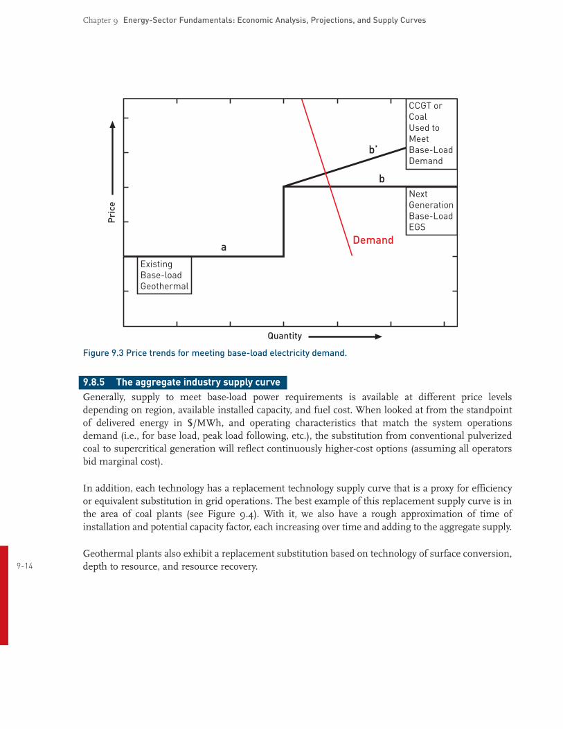
For baseload power, new additions to existing supplies can be added at relatively high cost in the short term. Generation and consequent fuel substitution is usually available to accomplish this (i.e., the substitution of gasfired combinedcycle plants usually reserved for load following can be brought in to satisfy baseload needs but at higher cost). This can represent a significant opportunity cost when the technology is more expensive at the margin.
As shown in Figure 9.3, for the installed base, the supply curve is elastic to the point where the operating capacity is fully utilized. Meeting additional demand will force new generation to come online. Where the new generation operates with baseload characteristics, it establishes a new elastic supply curve (slope b). Where the replacement is highercost loadfollowing technology, the supply curve is likely to assume normal market coefficients (slope b’).
Table 9.2 Permitting, siting, and construction relationships.
Generation Type Permitting, years Construction, years
Gas turbine 12 12
Renewable energy (wind, solar) 12 12
Renewable (biomass, MSW) 24 12
Renewable (geothermal) 12 23
Coal 23 23 913
Hydroelectric 56 610
Nuclear 410 210
Chapter 9 EnergySector Fundamentals: Economic Analysis, Projections, and Supply Curves
Next GenerationBase-LoadEGS
Quantity
Demanda
b
b’
Pri
ceCCGT orCoalUsed toMeetBase-LoadDemand
ExistingBase-loadGeothermal
Figure 9.3 Price trends for meeting baseload electricity demand.
9.8.5 The aggregate industry supply curve
Generally, supply to meet baseload power requirements is available at different price levels depending on region, available installed capacity, and fuel cost. When looked at from the standpoint of delivered energy in $/MWh, and operating characteristics that match the system operations demand (i.e., for base load, peak load following, etc.), the substitution from conventional pulverized coal to supercritical generation will reflect continuously highercost options (assuming all operators bid marginal cost).
In addition, each technology has a replacement technology supply curve that is a proxy for efficiency or equivalent substitution in grid operations. The best example of this replacement supply curve is in the area of coal plants (see Figure 9.4). With it, we also have a rough approximation of time of installation and potential capacity factor, each increasing over time and adding to the aggregate supply.
Geothermal plants also exhibit a replacement substitution based on technology of surface conversion, 914 depth to resource, and resource recovery.

Chapter 9 EnergySector Fundamentals: Economic Analysis, Projections, and Supply Curves
Quantity
Pri
cean
dEf
ficie
ncy
PulverizedCoal
AdvancedGasification
Supercritical
Figure 9.4 Schematic of replacement technology supply curve for coal plants.
9.8.6 Geothermal supply curve characteristics
By definition, the supply curve is a relation between each possible price of a given good and the quantity of that good that would be supplied for market sale at that price. This is typically represented as a graph showing the hypothetical supply of a product or service that would be available at different price points. The supply curve usually exhibits a positive slope, reflecting that higher prices give producers an incentive to supply more, in the hope of making greater revenue.
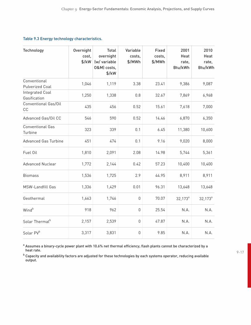
The supply of a “good” such as energy, either in the form of direct heat output or electricity, is dependent on the quality and quantity of the resource available, the technology used to extract it, and the cost of transforming it into a consumable product. Thus, the delivered cost of energy becomes a combination of capital (fixed) and fuel (variable) costs. When levelized over a period assumed to cover fixed costs and increased costs of operation, these technologies vary in terms of characteristics and delivered cost of energy as shown in Table 9.3.
Geothermal energy provides critical value to overall grid operations. While initial capital costs are 915
high, reliability and capacity factors are correspondingly high, with minimal downtime for maintenance and minimal fuel cost through replenishment of lost water in operations. The supply curve for energy from a geothermal system represents a combined range of production that is not traditional from the point of view of a normal economic good, where a price continuum represents the available supplies offered to the market. In this case, a singlewell complex represents a “system” of heat delivery and energy transformation. Essentially, the complex is “tuned” to “mine” a given heat resource through a range of depth represented by the well system, the fractured rock strata, and the amount of water that can be injected into the system to extract an optimal level of heat without degradation of the reservoir.

Chapter 9 EnergySector Fundamentals: Economic Analysis, Projections, and Supply Curves
Baseload needs are typically met by procuring the most inexpensive, nonvolatile, highcapacityfactor energy available. While this can vary by region or by time of day, in general, the most competitive fuel/technology combinations available to satisfy this demand include coal, hydroelectric, nuclear, and geothermal power. Dispatchability means that power can be generated when it is needed to meet peaksystem power loads. The primary metrics for dispatchability are the time when the peak load occurs, the length of the peakload period, and the capacity factor the system must maintain during these periods, exclusive of maintenance periods.
The use of geothermal energy in grid operations adds capacity to existing stock. In terms of capacity available for dispatch, the capacity factor is high. The primary responsibility of hydrothermal geothermal power is in baseload power delivery with very limited loadfollowing capability. However, power plants operating on EGS reservoirs should be much more flexible in following load because the circulation of the fluid through the hot rocks is controlled by pumping.
916
Chapter 9 EnergySector Fundamentals: Economic Analysis, Projections, and Supply Curves
Table 9.3 Energy technology characteristics.
Technology Overnight Total Variable Fixed 2001 2010
cost, overnight costs, costs, Heat Heat $/kW (w/ variable $/MWh $/MWh rate, rate,
O&M) costs, Btu/kWh Btu/kWh
$/kW
Conventional Pulverized Coal
1,046 1,119 3.38 23.41 9,386 9,087
Integrated Coal Gasification
1,250 1,338 0.8 32.67 7,869 6,968
Conventional Gas/Oil CC
435 456 0.52 15.61 7,618 7,000
Advanced Gas/Oil CC 546 590 0.52 14.46 6,870 6,350
Conventional Gas
Turbine 323 339 0.1 6.45 11,380 10,600
Advanced Gas Turbine 451 474 0.1 9.16 9,020 8,000
Fuel Oil 1,810 2,091 2.08 14.98 5,744 5,361
Advanced Nuclear 1,772 2,144 0.42 57.23 10,400 10,400
Biomass 1,536 1,725 2.9 44.95 8,911 8,911
MSWLandfill Gas 1,336 1,429 0.01 96.31 13,648 13,648
Geothermal 1,663 1,746 0 70.07 32,173a 32,173a
Windb 918 962 0 25.54 N.A. N.A.
Solar Thermalb 2,157 2,539 0 47.87 N.A. N.A.
Solar PVb 3,317 3,831 0 9.85 N.A. N.A.
a Assumes a binarycycle power plant with 10.6% net thermal efficiency; flash plants cannot be characterized by a heat rate. 917
b Capacity and availability factors are adjusted for these technologies by each systems operator, reducing available output.

Chapter 9 EnergySector Fundamentals: Economic Analysis, Projections, and Supply Curves
9.9 EGS Economic Models9.9.1 GETEM model description
The Geothermal Electric Technology Evaluation Model (GETEM) is a macromodel that estimates levelized cost of geothermal electric power in a commercial context. This model and its documentation were prepared as required work under a subcontract from the National Renewable Energy Laboratory (Golden, Colo.) to Princeton Energy Resources International (Rockville, Md.). Developed for the U.S. DOE Geothermal Technology Program, GETEM is coded in an Excel spreadsheet and simulates the economics of major components of geothermal systems and commercialdevelopment projects. The model uses a matrix of about 80 userdefined input variables to assign values to technical and economic parameters of a geothermal power project. In general categories, the variables account for geothermal resource characteristics, drilling and wellfield construction, power plant technologies, and development of geothermal power projects.
A key feature of the model is that GETEM uses a subset of the input matrix to apply change factors to model components. These factors are targeted to enable a user to investigate the impacts of diverse combinations of changes – ostensibly, improvements – in the performance and unit costs of a project. The impacts are quantified as net levelized energy costs.
GETEM accounts for the gamut of factors that comprise electric power costs – not prices – commonly referred to as “busbar costs.” GETEM applies documented and expertinterpreted conditions such as reservoir performance, drilling and construction costs, energy conversion factors, and competitive financial frameworks. It uses empirical, industrybased reference data. It is a good tool for evaluating casespecific costs, technology trends, cost sensitivities, and probabilistic values of technology goals. Thus, GETEM enables DOE to quantify the effectiveness of research program elements, using measures that reflect power industry practices.
9.9.2 Updated MIT EGS model “EGS Modeling for Windows” is a tool for economic analysis of geothermal systems. The software was based on work by Tester and Herzog (Tester et al., 1990; Tester and Herzog, 1991; Herzog et al., 1997) as enhanced by the MIT Energy Laboratory as part of its research into EGS systems sponsored by the Geothermal Technologies Office of the U.S. Department of Energy and further modified by Anderson (2006) as part of the assessment.
This model has been updated using the results of this study with regard to the cost of drilling, plant costs, stimulation costs, and the learningcurve analysis.
918 9.9.3 Base case and sensitivity
Table 9.4 lists the basecase parameters used in the evaluation of the levelized cost of electricity (LCOE) for three different stages of EGS technology: initial (today’s technology), midterm, and commercially mature. The plant capital costs, the well drilling and completion costs, and the stimulation costs are based on the results of the earlier chapters on those individual topics.
Chapter 9 EnergySector Fundamentals: Economic Analysis, Projections, and Supply Curves
Due to the uncertainty of the various rock drawdown models and the variations in rock characteristics across the United States, a drawdown parameter model (Armstead and Tester, 1987) was chosen to simulate the drawdown of the reservoir. The impedance per well is based on results from the Rosemanowes, Hijiori, and Soultz circulation tests. The debt and equity rates of return are based on the 1997 EERE Renewable Energy Technology Characterizations report (DOE, 1997).
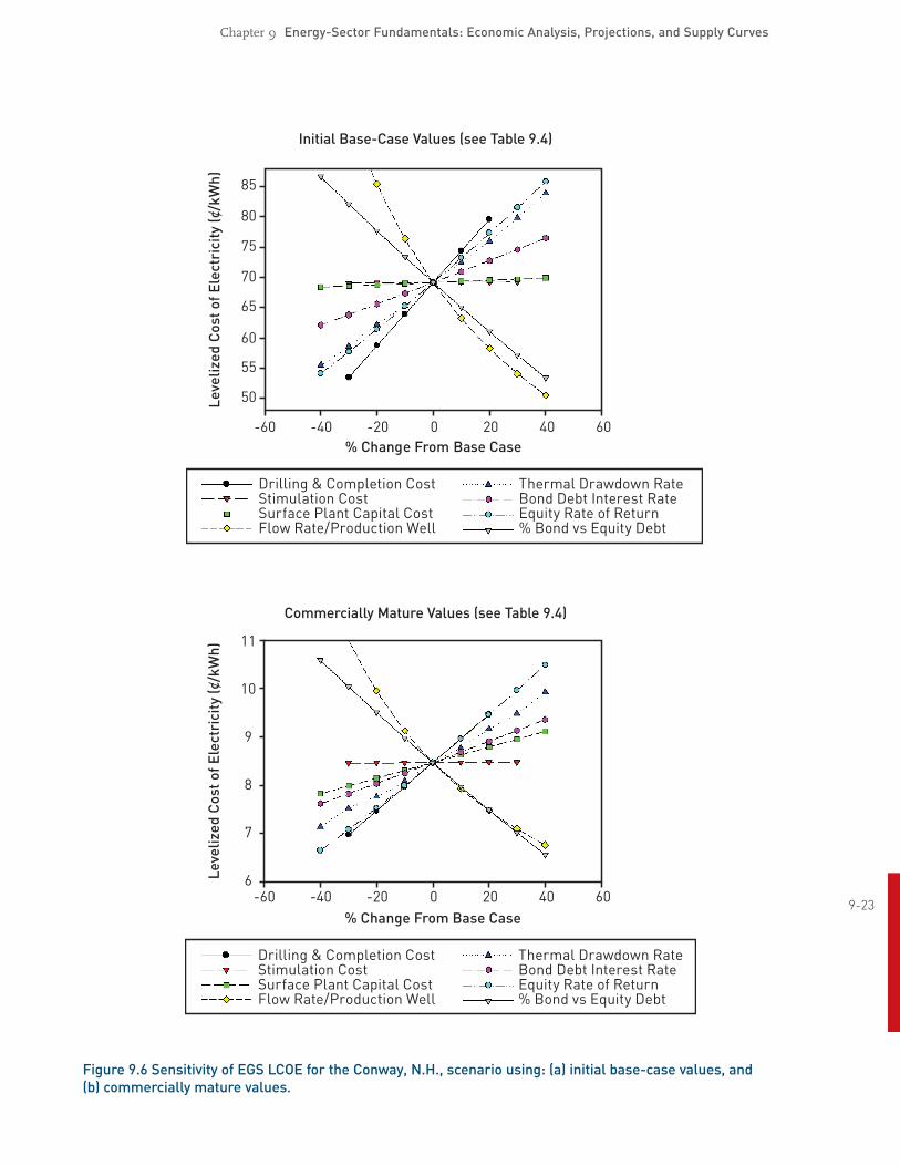
Table 9.5 shows the base case and optimized LCOE for the six sites selected in Chapter 4. The optimization was performed on the completion depth only, and the resulting electricity costs are at basecase conditions. Figures 9.5 and 9.6 illustrate the sensitivity of the levelized electricity costs to eight important reservoir, capital cost, and financial parameters in the MIT EGS model. Figure 9.6 depicts a highgrade prospect, whereas Figure 9.5 shows a lowgrade one. As one can discern from the sensitivity analysis, the cost of electricity is most sensitive to the geofluid flow rate, the drilling and completion costs, the thermal drawdown rate, as well as the economic parameters, debt/equity ratio, and the equity rate of return. The nonlinearity of the sensitivity of costs to drawdown rate is a result of the fixed plant lifetime of 30 years and the variability of the interval for reservoir rework/redrilling. Because a small fraction of the total capital cost is in the surface plant (in relation to the drilling cost), the LCOE is relatively insensitive to the surface plant costs for lowergrade resources (Figure 9.5), but the sensitivity increases for highergrade resources. Although sensitivity plots are shown here for the two extremes in geothermal gradient, the sensitivity at all six sites is shown in Appendix A.9.3.
919

Chapter 9 EnergySector Fundamentals: Economic Analysis, Projections, and Supply Curves
Table 9.4 Parameter values for the base case EGS economic models.
Parameter description Initial Values (today’s technology,
years 15)
Midterm Values
(years 511) Commercially
Mature Values
(years 20+)
Geofluid flow rate per producer 20 kg/s 40 kg/s 80 kg/s
Thermal drawdown rate 3 %/yr 3 %/yr 3 %/yr
Number of production wells per
injection well 2 23 3
Maximum allowable bottom hole 350°C 350°C 400°C
temperature
Average surface temperature 15°C 15°C 15°C
Impedance per well 0.15 MPa s/L 0.15 MPa s/L <0.15 MPa s/L
Temperature loss in production well 15°C 15°C 15°C
Water loss/total injected 2 % 2 % 1 %
Drawdown parameter (Armstead and Tester, 1987)
0.000119 kg/s.m2 0.000119 kg/s.m2 0.000119 kg/s.m2
Well deviation from vertical 0° 0° 0°
Well separation 500 m 500 m 500 m
Geofluid pump efficiency 80 % 80 % 80 %
Capacity factor 95 % 95 % 95 %
Fluid thermal availability drawdown
threshold before rework 20 % 20 % 20 %
Injection temperature 40°C 40°C 40°C
Well casing inner diameter 7” 7” 7”
Inflation rate 3 % 3 % 3 %
Debt rate of return 5.5 % 6.4 % 8.0 %
Equity rate of return N/A 17 % 17 %
Fraction of debt/equity 100/0 80/20 60/40
Plant lifetime 30 years 30 years 30 years
920 Property tax rate 2 % 2 % 2 %
Sales tax 6.5 % 6.5 % 6.5 %
Drilling contingency factor 20 % 20 % 20 %

Chapter 9 EnergySector Fundamentals: Economic Analysis, Projections, and Supply Curves
Table 9.5 Levelized cost of electricity (LCOE) for six selected sites for development.
LCOE Using Initial Optimized LCOE Using Site ∂T/∂z Depth to Completion Fracture Costs Values for Base Case Commercially Mature (°C/km)Name Granite Depth ($K)
(¢/kWh) Values (¢/kWh) (km) |(km)
@@ DepthMIT EGS GETEM MIT EGS GETEM
180 l/s93 l/s (km)
East Texas 40 5 5 145 171 29.5 21.7 6.2 5.8 7.1
Basin
Nampa 43 4.5 5 260 356 24.5 19.5 5.9 5.5 6.6
Three
Sisters 50 3.5 5 348 450 17.5 15.7 5.2 4.9 5.1
Area
Poplar 55 4 2.2 152 179 74.7 104.9 5.9 4.1 4.0
Dome a
Poplar 37 4 6.5 152 179 26.9 22.3 5.9 4.1 4.0
Dome b
Clear 67 3 5 450 491 10.3 12.7 3.6 4.1 5.1
Lake
Conway 26 0 7 502 580 68.0 34.0 9.2 8.3 10*
Granite
*10 km limit put on drilling depth – MITEGS LCOE reaches 7.3 ¢/kWh at 12.7 km and 350°C geofluid temperature.
We have created a series of sensitivity graphs to illustrate the sensitivity of the levelized electricity costs to eight important reservoir, capital cost, and financial parameters in the MIT EGS model. The first graph illustrates the base case itself, and the following tables illustrate the range of difference both by location and by changes in the key characteristic of flow rates.
921

Chapter 9 EnergySector Fundamentals: Economic Analysis, Projections, and Supply Curves
Initial BaseCase Values (see Table 9.4)
% Change From Base Case-60 -40 -20 0 20 40 60
8
9
10
11
12
13
14
Thermal Drawdown RateBond Debt Interest RateEquity Rate of Return% Bond vs Equity Debt
Drilling & Completion CostStimulation CostSurface Plant Capital CostFlow Rate/Production Well
Leve
lized
Cos
tofE
lect
rici
ty(c
/kW
h)
Commercially Mature Values (see Table 9.4)
922 % Change From Base Case
-60
3.0
3.5
4.0
4.5
-40 -20 0 20 40 60
Thermal Drawdown RateBond Debt Interest RateEquity Rate of Return% Bond vs Equity Debt
Drilling & Completion CostStimulation CostSurface Plant Capital CostFlow Rate/Production Well
Leve
lized
Cos
tofE
lect
rici
ty(c
/kW
h)
Figure 9.5 Sensitivity of EGS LCOE for the Clear Lake (Kelseyville, Calif.) scenario using: (a) initial basecase values, and (b) commercially mature values.
Chapter 9 EnergySector Fundamentals: Economic Analysis, Projections, and Supply Curves
Initial BaseCase Values (see Table 9.4)
% Change From Base Case-60 -40 -20 0 20 40 60
50
55
60
65
70
75
80
85
Thermal Drawdown RateBond Debt Interest RateEquity Rate of Return% Bond vs Equity Debt
Drilling & Completion CostStimulation CostSurface Plant Capital CostFlow Rate/Production Well
Leve
lized
Cos
tofE
lect
rici
ty(c
/kW
h)
Commercially Mature Values (see Table 9.4)
923 % Change From Base Case
-60 -40 -20 0 20 40 606
7
8
9
10
11
Thermal Drawdown RateBond Debt Interest RateEquity Rate of Return% Bond vs Equity Debt
Drilling & Completion CostStimulation CostSurface Plant Capital CostFlow Rate/Production Well
Leve
lized
Cos
tofE
lect
rici
ty(c
/kW
h)
Figure 9.6 Sensitivity of EGS LCOE for the Conway, N.H., scenario using: (a) initial basecase values, and (b) commercially mature values.

924
Chapter 9 EnergySector Fundamentals: Economic Analysis, Projections, and Supply Curves
9.10 Supply Curves and Model ResultsToday, geothermal power is considered baseload capacity because it is fully available yearround, 24 hours a day. A utility could use a baseload supply curve for planning purposes in one of two ways. They can determine how much renewable baseload capacity they might buy for a certain price, and they can see what they would have to pay for capacity equal to their needs.
The supply of power available from current and future generating facilities is, by definition, a reflection of access to heat reserves. The heat reserves, in turn, are accessible only as drilling and fracturing techniques are improved and demonstrated to be economically competitive.
The North American continent and, by definition, the United States, is underlain by a vast heat resource varying in heat and consequent power potential as a function of depth and transmissivity. The supply of energy available can be portrayed in a variety of ways, each reflecting technology and access over time.
The ultimate resource is virtually infinite, but inaccessible. That is, if it were possible to drill to depths where >350°C heat stores were available, fracture the rock at that depth, and gain access to reservoirs created as a result, then all basement rock on the continent would be a source of EGS. As a practical matter, this is not likely to occur within the next 50 years, so we have arbitrarily limited the estimates of available energy by assuming aggressive, but historically proven, learning and technology application scenarios.
Modeling a resource with infinite capacity requires arbitrary assumptions on the resource recovery. We can access relatively shallow resources with hydrothermal electric technologies and drilling techniques, which effectively defines current technology. Expansion and exploration into new land areas with these technologies offers the first example of a longterm supply curve, which expands to satisfy demand as a function of applying new capital with existing technology and expands the supply curve outward.
As technology and drilling techniques improve, access to deeper and more productive reserves become available.16 This can be described by dividing the total resource available at depths shallower than 3 km for nearterm development and the remaining muchlarger resource at depths greater than 3 km for longterm development.
Technically, it is impossible to know how large the unidentified EGS resource might be. Muffler and Guffanti (1979) and Renner et al. (1975) speculate that this unidentified hydrothermal resource could be anything from twice to five times the identified resource. An ongoing study by Petty and others (Petty and Porro, 2006) also estimates the EGS portion of the geothermal supply.
The result can be illustrated by a set of supply curves that describe the available resource over time. These curves demonstrate how the available EGS resource is being utilized with incremental access to it, starting as an expansion of existing, highgrade hydrothermal resources and ending with lowgrade conductiondominated basement rock EGS resources at depths greater than 3 km.
Chapter 9 EnergySector Fundamentals: Economic Analysis, Projections, and Supply Curves
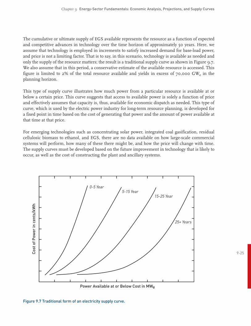
The cumulative or ultimate supply of EGS available represents the resource as a function of expected and competitive advances in technology over the time horizon of approximately 50 years. Here, we assume that technology is employed in increments to satisfy increased demand for baseload power, and price is not a limiting factor. That is to say, in this scenario, technology is available as needed and only the supply of the resource matters; the result is a traditional supply curve as shown in Figure 9.7. We also assume that in this period, a conservative estimate of the available resource is accessed. This figure is limited to 2% of the total resource available and yields in excess of 70,000 GWe in the planning horizon.
This type of supply curve illustrates how much power from a particular resource is available at or below a certain price. This curve suggests that access to available power is solely a function of price and effectively assumes that capacity is, thus, available for economic dispatch as needed. This type of curve, which is used by the electric power industry for longterm resource planning, is developed for a fixed point in time based on the cost of generating that power and the amount of power available at that time at that price.
For emerging technologies such as concentrating solar power, integrated coal gasification, residual cellulosic biomass to ethanol, and EGS, there are no data available on how largescale commercial systems will perform, how many of these there might be, and how the price will change with time. The supply curves must be developed based on the future improvement in technology that is likely to occur, as well as the cost of constructing the plant and ancillary systems.
925
Power Available at or Below Cost in MW
0-5 Year5-15 Year
15-25 Year
25+ Years
Cos
tofP
ower
ince
nts/
kWh
e
Figure 9.7 Traditional form of an electricity supply curve.
Chapter 9 EnergySector Fundamentals: Economic Analysis, Projections, and Supply Curves
9.10.1 Supply of EGS power on the edges of existing hydrothermal systems
As geothermal developers drill outward away from the best and most permeable parts of current highgrade hydrothermal fields, they often encounter rock that has high temperatures at similar or deeper depths than the main field, but with lower natural permeability. It is becoming routine for geothermal developers to stimulate these lower permeability wells to increase fluid production rates up to commercial levels. Pumping large volumes of cold water at high rates over a short period, treating with acid, or injecting cold water at lower rates for a long period all are regularly used to try to improve well productivity on the edges of hydrothermal systems. However, this is most successful when the stimulated wells are in hydrologic connection with the wells in the main part of the reservoir. When the lower permeability well is not connected to the main reservoir, it and the associated hightemperature rock reservoir can be treated as a separate EGS project. For instance, Well 231 at Desert Peak in Nevada is of this type and is currently part of a U.S. DOEsponsored EGS research study. It may be possible to stimulate the Desert Peak well, drill production wells around it, and create a viable EGS reservoir.
In other areas, a hydrothermal resource has been identified, but it is not permeable enough to be commercial, and so is not being developed. The EGS resources in these lowpermeability hydrothermal areas and on the edges of identified hydrothermal systems could be considered “identified” EGS systems. They are likely to be developed earlier than the deeper EGS systems because they tend to be associated with high conductive gradients instead of convective temperature anomalies. Because the hydrothermal sites have been identified in USGS Circular 790 (Muffler and Guffanti, 1979) with updates by Petty et al., (1991), the associated EGS resource could be calculated by subtracting the fraction of the hydrothermal resource deemed commercial in the near term from the totals found as part of these earlier studies. It is assumed that these noncommercial resources will require stimulation to produce at commercial rates before they can be considered EGS resources.
While the reserves of recoverable energy in these identified EGS resources can be assessed in the same way that a hydrothermal system is assessed – by a volumetric heat calculation – there is probably an equal or greater “unidentified” EGS resource associated with convective temperature anomalies that have not been discovered yet. Because the resourcebase estimates in our study start at a depth of 3 km, the identified and unidentified EGS resource associated with existing hydrothermal resources are not included in this calculated reserve. For this reason, the identified and unidentified EGS resource was calculated separately.
Using a costing code (GETEM) (see Section 9.9.1), the forecast cost of power was calculated based on current capabilities in EGS technology with the specific temperatures and depths for each identified resource. Each of these identified EGS resources has a depth and temperature based on the data
926 available from the hydrothermal resource associated with it, or one similar to it, if there is no associated resource. Flow rates were based on the current bestavailable flow from the longest test at the Soultz projects, which has produced the highest observed sustained production flow rates from an EGS reservoir. The available power was then ranked by cost and a cumulative amount of power plotted against the associated cost of power. The result is a forecast total supply curve shown in Figure 9.8. This supply curve assumes that technology is applied as needed, in response to competitivemarket signals to deliver power for dispatch in the existing system. It is simplistic in the assumption that there are no limits to transmission or available land sites beyond the restrictions of public parks, military, or existing urban facilities.

Chapter 9 EnergySector Fundamentals: Economic Analysis, Projections, and Supply Curves
Power Available at or Below Cost in MW
0
5
10
15
20
25
30
35
40
45
50
Cos
tofP
ower
(cen
ts/k
Wh)
0 5000 10000 15000 20000 25000
2004 US$
Base5yr15yr25yr35yr
e
Figure 9.8 Predicted supply curves using the GETEM model for identified EGS sites associated withhydrothermal resources at depths shallower than 3 km. The base case corresponds to today’s technologyand the 5, 15, 25, and 35year values correspond to the state of technology at that number of years intothe future.
The GETEM code also allows the user to change cost multipliers to calculate the impact of technologyimprovement. To look at the future cost of power from the identified EGS resources, the researchtargets from drilling, conversion, and EGS research sponsored by the federal government were usedas multipliers in the GETEM code. The future cost of power was also calculated based on both thelearning experience expected from the longterm test upcoming at Soultz, Cooper Basin, and otherEGS projects, as well as on the projected improvements from the DOE Geothermal strategic plan andthe multiyear program plan. These cost multipliers were entered into the GETEM code to calculate a5, 15, 25, and 35year cost of power. Of course, the magnitude of cost improvements in the long termare highly speculative and depend on achievements from a continuing aggressive R&D program, bothin the United States and in other countries.
9.10.2 Supply of EGS power from conductive heating 927
The EGS thermal resource described in Chapter 2 is due primarily to conductiondominated effectsat depths below 3 km. This resource is more evenly distributed throughout the United States thangeothermal resources that are naturally correlated with hydrothermal anomalies. Starting from theheatinplace calculations described in Chapter 2, the accessible and recoverable heat were calculatedand converted to electric power for each depth and average temperature. This allows us to use theGETEM costing code with the depth and temperature as input with current technology and the costfor fracturing determined for this study to produce a supply curve for the entire United States (Figure9.9). The assumption used for the flow rate in the current supply curve is based on the flow rate

Chapter 9 EnergySector Fundamentals: Economic Analysis, Projections, and Supply Curves
achieved during the longest flow test at the Soultz project. The fracturing cost used in the model runs is twice the average of the costs shown in Table 5.2 (Chapter 5), approximately $700,000. The other inputs for GETEM were assumed to be similar to current technology as demonstrated at the Soultz project. For the fiveyear costs, the goals of the U.S. DOE Geothermal Technology Program MYPP were used, along with the assumption that the Soultz longterm test will be successful at maintaining 50 kg/s flow for an extended time period.
The supply curve shown in Figure 9.9 provides an estimate of the electric power capacity potentially available assuming a 30year project life (xaxis), at or below a cost in thirdquarter 2004 dollars shown on the yaxis. It illustrates the shift likely from small increases in baseload power contract prices. Figure 9.9 shows the dramatic influence on the price expected, given improvements in technology and more extensive field experience.
Base CostIncremental improvements
Supply Curve for EGS Power in the United States
Developable Power over 30 Years (GW )
Cos
t(ce
nts/
kWh)
0 20001000 4000 6000 80003000 5000 7000 9000 100000
10
20
30
40
60
50
70
e
Figure 9.9 Supply of developable power from conductive EGS sources at depths greater than 3 km at cost of energy calculated using GETEM model for base case as shown in Table 9.4. This includes incremental improvements only from DOE Geothermal Technology Program Multiyear Plan.
928 9.10.3 Effects of learning on supply curves
A second type of supply curve illustrates the effect of increased knowledge of the resource and applications of technology needed to recover it. The learning curve process is illustrated in Figure 9.10, showing the increased efficiency on a fieldbyfield basis (field learning) and the cumulative effect on the installed base of power systems (technology learning) capacity.
Applying this learning curve to satisfy market demand assumes access to land and transmission facilities where power can be delivered to markets. For analytic purposes, we assume that this can be modeled as a dynamic but orderly increase in available supplies when the resource is competitively

Chapter 9 EnergySector Fundamentals: Economic Analysis, Projections, and Supply Curves
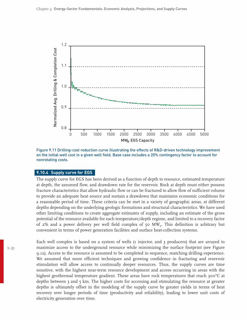
priced. This supply relationship is shown in Figure 9.11 and demonstrates the dynamic effects of field information and drilling experience, as well as the benefits of applying new technologies as power projects are developed. Here, the combination of increased drilling depth, diminished drilling cost, increased fracture, and consequent flow rate enable increased cumulative installed capacity.
0.6
0.9
0.7
0.8
1.0
1.1
1.2
Well Field 1 Well Field 2 Well Field 3
Individual Well CostAverage Well Cost
Nor
mal
ized
Dri
llin
g&
Com
plet
ion
Cos
ts
Figure 9.10 Drillingcost learning curve illustrating the learning process that occurs within each well field. Base case includes a 20% contingency factor to account for nonrotating costs.
929
Chapter 9 EnergySector Fundamentals: Economic Analysis, Projections, and Supply Curves
0.8
1.1
0.9
1.0
1.2
MW EGS Capacity0 500 1000 1500 2000 2500 3000 3500 4000 4500 5000
Nor
mal
ized
Avg.
Dri
llin
g&
Com
plet
ion
Cos
t
e
Figure 9.11 Drillingcost reduction curve illustrating the effects of R&Ddriven technology improvement on the initial well cost in a given well field. Base case includes a 20% contingency factor to account for nonrotating costs.
9.10.4 Supply curve for EGS
The supply curve for EGS has been derived as a function of depth to resource, estimated temperature at depth, the assumed flow, and drawdown rate for the reservoir. Rock at depth must either possess fracture characteristics that allow hydraulic flow or can be fractured to allow flow of sufficient volume to provide an adequate heat source and sustain a drawdown that maintains economic conditions for a reasonable period of time. These criteria can be met in a variety of geographic areas, at different depths depending on the underlying geologic formations and structural characteristics. We have used other limiting conditions to create aggregate estimates of supply, including an estimate of the gross potential of the resource available for each temperature/depth regime, and limited to a recovery factor of 2% and a power delivery per well field complex of 50 MWe. This definition is arbitrary but convenient in terms of power generation facilities and surface heatcollection systems.
Each well complex is based on a system of wells (1 injector, and 3 producers) that are arrayed to
930 maximize access to the underground resource while minimizing the surface footprint (see Figure 9.12). Access to the resource is assumed to be completed in sequence, matching drilling experience. We assumed that more efficient techniques and growing confidence in fracturing and reservoir stimulation will allow access to continually deeper resources. Thus, the supply curves are time sensitive, with the highest nearterm resource development and access occurring in areas with the highest geothermal temperature gradient. These areas have rock temperatures that reach 300°C at depths between 3 and 5 km. The higher costs for accessing and stimulating the resource at greater depths is ultimately offset in the modeling of the supply curve by greater yields in terms of heat recovery over longer periods of time (productivity and reliability), leading to lower unit costs of electricity generation over time.

Chapter 9 EnergySector Fundamentals: Economic Analysis, Projections, and Supply Curves
Injection well
Production wells
Fracture zones
Elevation view
Ground surface
Plan view
Figure 9.12 Schematic of the quartet wellfield complex and expected fracture stimulation zones at intervals.
9.10.5 EGS well characteristics
For development of the supply curves, we have assumed that production wells are drilled in triplets and complexes that yield approximately 50 MWe of baseload power and are arrayed in modules that optimize yield from the entire resource base as a function of depth and temperature. We have assumed fracture and stimulation of zones around the corresponding well depth that have an average radius of 500 meters and a swept area of 5,000 m2 per fracture zone. This is illustrated in Figure 9.12 for a quartet configuration. A well complex producing 50 MWe would have between 30 and 40 wells, depending on subsurface conditions.
9.11 Learning Curves and Supply CurvesAssuming that sufficient R&D funds have supported a successful deployment of several firstgeneration EGS plants, the stage is set for commercial development of EGS, where learning effects will influence costs. Accessing proportionally larger amounts of the EGS resource base is expected to 931 result in greater economies of scale for delivered power. This will translate into lower average costs per well as a function not only of wells drilled per field, but wells drilled regionally as well. This learning curve concept has been assessed and applied for almost three decades in oil and gas drilling (Ikoku, 1978; Brett and Millheim, 1986) as well as across a number of energy conversion technologies (McDonald and Schrattenholzer, 2001). We have assumed a cost reduction of 5% per well through the first five wells in a complex, with 1% per well for the next five wells, and constant drilling costs beyond that point – a cost reduction realized through the decrease in “trouble” (Kravis et al., 2004) (see Figure 9.13). This sequence is likely to be repeated in new complexes with a maximum reduction in expected drilling costs of 25% overall through the life of the well complex. Because each well is

Chapter 9 EnergySector Fundamentals: Economic Analysis, Projections, and Supply Curves
expected to be redrilled or improved three times during its lifetime, the cost reduction applies to the total capital cost of the well through the lifetime, because knowledge gained in the initial drilling will be transferred to future exploration.
Number of Wells Drilled in Formation
00.70
0.75
0.80
0.85
0.90
0.95
1.00
1.05
2 4 6 8 10
Frac
tion
ofB
ase
Cas
eC
ost
Figure 9.13 Learning curve influence on drilling cost.
A similar learning curve is expected for fracturing and stimulation costs, plant capital expenditures, plant and wellfield O&M costs, and exploration success (see Table 9.6 and Figure 9.14). Learning curves are modeled using the following functional form:
(912)
where
CMW
932 MWcum = Cumulative EGS capacity installed under various supply scenarios
ref = Reference installed capacity for which cost is reliably known
i = empirical fitted parameters in Eq. (912) that are correlated to specific learning
CCC
curve behavior
1 = Technical limit achievable
2 = Learning potential
3 = Learning rate.
Chapter 9 EnergySector Fundamentals: Economic Analysis, Projections, and Supply Curves
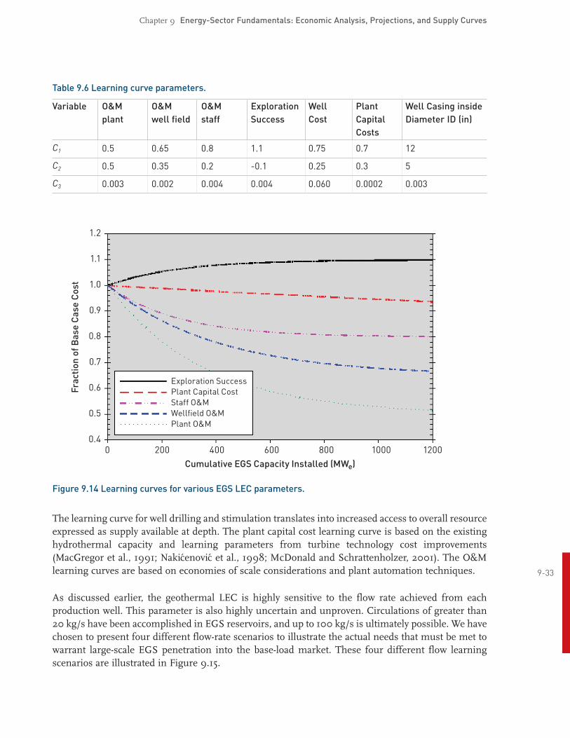
Table 9.6 Learning curve parameters.
Variable O&M O&M O&M Exploration Well Plant Well Casing inside
plant well field staff Success Cost Capital Diameter ID (in) Costs
C1 0.5 0.65 0.8 1.1 0.75 0.7 12
C2 0.5 0.35 0.2 0.1 0.25 0.3 5
C3 0.003 0.002 0.004 0.004 0.060 0.0002 0.003
Cumulative EGS Capacity Installed (MW )
Exploration SuccessPlant Capital CostStaff O&MWellfield O&MPlant O&M
0 200 400 600 800 1000 12000.4
0.5
0.6
0.7
0.8
0.9
1.0
1.1
1.2
Frac
tion
ofB
ase
Cas
eC
ost
e
Figure 9.14 Learning curves for various EGS LEC parameters.
The learning curve for well drilling and stimulation translates into increased access to overall resource expressed as supply available at depth. The plant capital cost learning curve is based on the existing hydrothermal capacity and learning parameters from turbine technology cost improvements (MacGregor et al., 1991; Nakicenovic et al., 1998; McDonald and Schrattenholzer, 2001). The O&M learning curves are based on economies of scale considerations and plant automation techniques. 933
As discussed earlier, the geothermal LEC is highly sensitive to the flow rate achieved from each production well. This parameter is also highly uncertain and unproven. Circulations of greater than 20 kg/s have been accomplished in EGS reservoirs, and up to 100 kg/s is ultimately possible. We have chosen to present four different flowrate scenarios to illustrate the actual needs that must be met to warrant largescale EGS penetration into the baseload market. These four different flow learning scenarios are illustrated in Figure 9.15.

Chapter 9 EnergySector Fundamentals: Economic Analysis, Projections, and Supply Curves
Cumulative EGS Capacity Installed (MW )
100kg/s – Fast Growth100kg/s – Slow Growth80kg/s60kg/s
Flow Rate Technical Limits
0 200 400 600 800 1000 12000
20
40
60
80
100
120
Flow
Rat
epe
rP
rodu
ctio
nW
ell(
kg/s
)
e
Figure 9.15 Learning curves for production well flow rates.
Power generation is extremely capitalintensive at inception and tends to be fuel or variablecost sensitive over time. Once a power system is organized around a suite of technologies, such as fossilbased generation, it becomes difficult to shift or redesign the system. Key reasons for this can be found in the nature of the support facilities, including fuel acquisition and transformation, transportation pipes and wires, storage facilities, and delivery systems – which also entail longlived capitalintensive facilities. As a consequence, improvements of existing systems tend to occur at the margin, in the form of advanced technologies for a particular fuel source.
Geothermal power technologies are no exception to this trend. The learning curve involved in extending drilling capability, and in more efficient fracture and stimulation of rock, leads directly to higher rates of heat recovery. The three phases of expected improvement demonstrate the application of the learning curve thesis in terms of more efficient power generation and lower costs. The fact that the delivered cost of power remains effectively level over time after taking advantage of installation economies, e.g., largersize plants, demonstrates the benefits of continuous improvement in techniques and technology. Renewable energy technologies, in particular, have shown great benefit
934 from focused research and development programs, which can significantly shorten the time of successful market penetration and adoption (Moore and Arent, 2006).

Chapter 9 EnergySector Fundamentals: Economic Analysis, Projections, and Supply Curves
9.12 Forecast Supply of Geothermal Energy“Getting a new idea adopted, even when it has obvious advantages, is difficult. Many innovations require a lengthy period of many years from the time when they become available to the time when they are widely adopted. Therefore, a common problem for many individuals and organizations is how to speed up the rate of diffusion of an innovation.” (Rogers, 2003)
In this section, we describe the forecast of supply as a function of resource and market price in various scenarios and sensitivity ranges. The basis of all of the learning curve benefits described earlier is the actual installation of EGS power. Therefore, we must establish a marketpenetration plan that would allow for these benefits to be realized. Diffusion of an innovation follows a normal bell distribution (Rogers, 2003):
(913)
This normal distribution gives the installation rate for EGS in our evaluation. Equation (913) is centered on time tmax, where the EGS installation rate would be at a maximum. According to the Rogers diffusion theory, the standard deviation, , categorizes the adopters into: (i) innovators (tmax–3 ≤ t ≤ tmax–2 ), (ii) early adopters (tmax –2 ≤ t ≤ tmax– ), (iii) early majority (tmax – t
≤ t ≤ max), (iv) late majority (tmax ≤ t ≤ tmax+ ), and (v) laggards (tmax+ ≤ t) 17. We must also normalize
Eq. (913) by the total possible installed EGS capacity, MWtot,EGS to scale up to the desired installed capacity. When Eq. (913) is integrated with respect to time, we get the cumulative capacity of EGS. Both the total capacity and tmax are determined iteratively, depending on the baseload market and the EGS LEC. The parameters tmax and were determined iteratively considering the economics of the innovation. The categorical divisions, given by MW
, were found to be 10 years, tmax = 40 years, and
tot,EGS (t = 50yrs) = 100,000 MWe, per the scope of this project. Using these parameters, we plot the distribution of installation rate and the cumulative EGS capacity in Figure 9.16. This distribution is used throughout the remaining analysis and is verified with the market considerations in the sections to follow. Using this scenario, one can see that the innovators enter the market at year 10, the early adopters at year 20, and the early majority at year 30. As will be seen in the following sections, the innovators enter the market once parity with market baseload price is reached, while the late majority adopt the technology following the period of highest profitability.
935

Chapter 9 EnergySector Fundamentals: Economic Analysis, Projections, and Supply Curves
Year
Installation RateCumulative Capacity
00
10 20 30 40 50
1000
2000
3000
4000
5000
0
20000
40000
60000
80000
100000
EGS
Inst
alla
tion
Rat
e(M
W/y
r)e
Cum
ulat
ive
Inst
alle
dEG
SC
apac
ity
(MW
)e
Figure 9.16 Diffusion of technology scenario – 100,000 MWe after 50 years.
9.12.1 The role of technology
Because technology improvements will improve the ability to access new and deeper areas with predictably higher heat content (Armstead and Tester, 1987), we can develop a proxy for new supply curve(s), represented by access to the deeper resources. We expect technology improvements in surface plants to decrease the delivered cost of energy (COE), by allowing higher efficiency energy conversion from heat to electricity, effectively utilizing lowergrade heat content areas that are accessible at shallower depths.
Using both the GETEM and the MIT EGS models, we have forecast the relationship of new energy supplies to the COE delivered to the expected baseload power market. The price of energy falls predictably with higher volumes of installed capacity, finally approaching a breakeven price at approximately 11 years from inception; this is shown in section 9.12.2. The effect of technology and subsequent price levels is sensitive to assumptions in the models regarding fixed rates of return vs. variable rates in ultimately achieving performance goals. We have illustrated both approaches in this
936 research and they are reflected in the graphs shown later in this chapter.
The key to decreasing installed costs is an investment in key areas identified above, including drilling techniques, subsurface analysis, rock fracture, flow control, wellfield monitoring, and injection mechanics. This implies an ongoing investment in research and development, including a proofofconcept design to access deeper resources and higher heat regimes. The R&D equivalent commitment can be measured as “absorbed cost,” which is a proxy for the subsidy that would represent industry investment in capital, land, and support facilities needed to produce the first 240 MWe of delivered power.
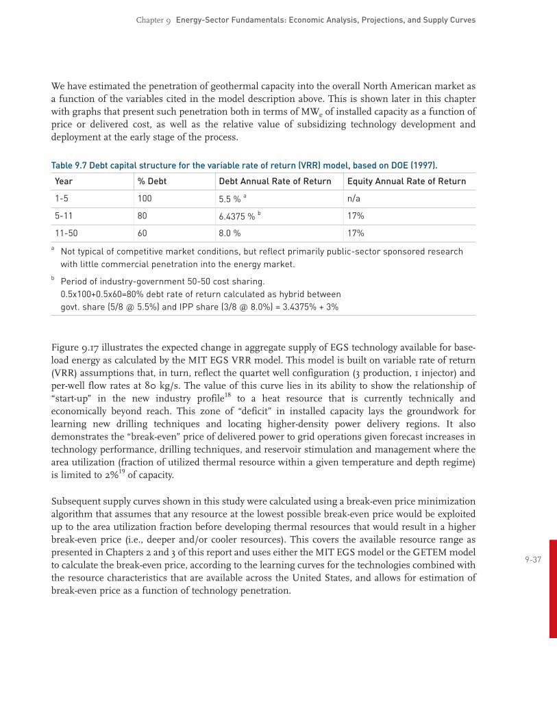
Chapter 9 EnergySector Fundamentals: Economic Analysis, Projections, and Supply Curves
We have estimated the penetration of geothermal capacity into the overall North American market as a function of the variables cited in the model description above. This is shown later in this chapter with graphs that present such penetration both in terms of MWe of installed capacity as a function of price or delivered cost, as well as the relative value of subsidizing technology development and deployment at the early stage of the process.
Table 9.7 Debt capital structure for the variable rate of return (VRR) model, based on DOE (1997).
Year % Debt Debt Annual Rate of Return Equity Annual Rate of Return
15 100 n/a5.5 % a
511 80 17%6.4375 % b
1150 60 8.0 % 17%
a Not typical of competitive market conditions, but reflect primarily publicsector sponsored research
with little commercial penetration into the energy market. b Period of industrygovernment 5050 cost sharing.
0.5x100+0.5x60=80% debt rate of return calculated as hybrid between govt. share (5/8 @ 5.5%) and IPP share (3/8 @ 8.0%) = 3.4375% + 3%
Figure 9.17 illustrates the expected change in aggregate supply of EGS technology available for baseload energy as calculated by the MIT EGS VRR model. This model is built on variable rate of return (VRR) assumptions that, in turn, reflect the quartet well configuration (3 production, 1 injector) and perwell flow rates at 80 kg/s. The value of this curve lies in its ability to show the relationship of “startup” in the new industry profile18 to a heat resource that is currently technically and economically beyond reach. This zone of “deficit” in installed capacity lays the groundwork for learning new drilling techniques and locating higherdensity power delivery regions. It also demonstrates the “breakeven” price of delivered power to grid operations given forecast increases in technology performance, drilling techniques, and reservoir stimulation and management where the area utilization (fraction of utilized thermal resource within a given temperature and depth regime) is limited to 2%19 of capacity.
Subsequent supply curves shown in this study were calculated using a breakeven price minimization algorithm that assumes that any resource at the lowest possible breakeven price would be exploited up to the area utilization fraction before developing thermal resources that would result in a higher breakeven price (i.e., deeper and/or cooler resources). This covers the available resource range as presented in Chapters 2 and 3 of this report and uses either the MIT EGS model or the GETEM model
937to calculate the breakeven price, according to the learning curves for the technologies combined with the resource characteristics that are available across the United States, and allows for estimation of breakeven price as a function of technology penetration.
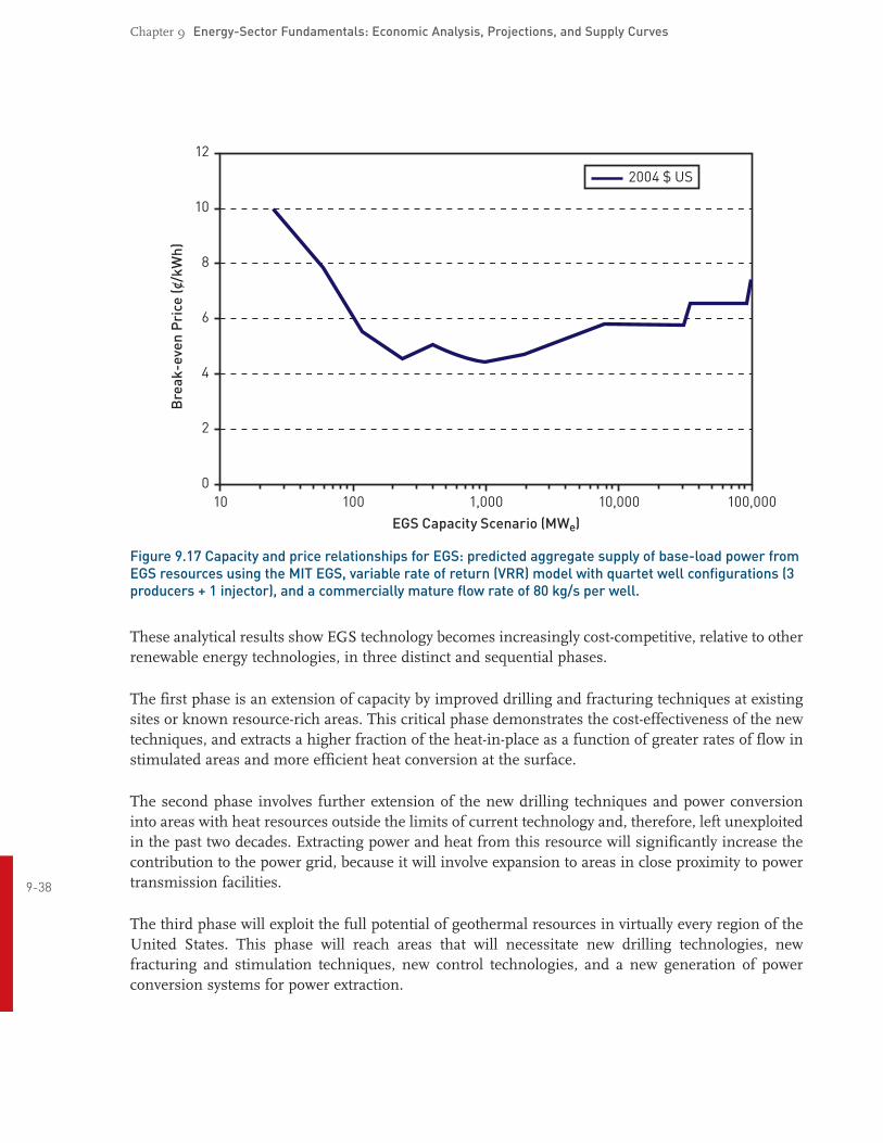
Chapter 9 EnergySector Fundamentals: Economic Analysis, Projections, and Supply Curves
EGS Capacity Scenario (MWe)
2004 $ US
0
2
4
6
8
10
12
10 100 1,000 10,000 100,000
Bre
ak-e
ven
Pri
ce(c
/kW
h)
Figure 9.17 Capacity and price relationships for EGS: predicted aggregate supply of baseload power from EGS resources using the MIT EGS, variable rate of return (VRR) model with quartet well configurations (3 producers + 1 injector), and a commercially mature flow rate of 80 kg/s per well.
These analytical results show EGS technology becomes increasingly costcompetitive, relative to other renewable energy technologies, in three distinct and sequential phases.
The first phase is an extension of capacity by improved drilling and fracturing techniques at existing sites or known resourcerich areas. This critical phase demonstrates the costeffectiveness of the new techniques, and extracts a higher fraction of the heatinplace as a function of greater rates of flow in stimulated areas and more efficient heat conversion at the surface.
The second phase involves further extension of the new drilling techniques and power conversion into areas with heat resources outside the limits of current technology and, therefore, left unexploited in the past two decades. Extracting power and heat from this resource will significantly increase the contribution to the power grid, because it will involve expansion to areas in close proximity to power
938 transmission facilities.
The third phase will exploit the full potential of geothermal resources in virtually every region of the United States. This phase will reach areas that will necessitate new drilling technologies, new fracturing and stimulation techniques, new control technologies, and a new generation of power conversion systems for power extraction.

Chapter 9 EnergySector Fundamentals: Economic Analysis, Projections, and Supply Curves
9.12.2 Variable debt/equity rates vs. fixed charge rates (FCRs) Most energy models adopt either fixed or variable charge ratebased scenarios. Fixed charge rates include a range of factors such as construction financing, financing fees, return on debt and equity, depreciation, income tax, property tax, and insurance. The fixed charge rate, when multiplied by the cost of a new construction project, yields the annual “fixed charges.” Thus, the fixed charges are the annual interest expenses of the money borrowed to build, plus the annual costs to operate and maintain a new construction project. This is in contrast to the variable cost rate charge, which shows what any given loan fund needs to yield to cover variable costs. Here,
(914)
Fixed charge rate comparison for renewable technologies is a common procedure and allows comparison across technologies. We have adopted the 12.8% fixed charged rate cited in the National Energy Modeling System (NEMS) model, sponsored by DOE, as our fixed charge rate for calculations. This is used consistently in both the GETEM and MIT EGS models.
Although all results from either the GETEM or the MIT EGS model show the cost of energy declining to a point below competitive alternatives and are in general agreement in terms of overall cumulative supply, the use of VRR in MIT EGS offers what we believe is a closer approximation of market conditions when used in the case of developing technologies as opposed to commercially mature, established technologies.
A comparison of the two approaches will illustrate this effect. The results can be dramatic as shown in Figure 9.18. In Figure 9.18b, the levelized energy costs are significantly lower when using a fixed charge rate opposed to using a variable rate of return as in Figure 9.18a, holding other model parameters constant.
A key result that emerged between the use of variable cost and fixed cost models is illustrated by comparing Figure 9.18a and Figure 9.19a. Here, both scenarios achieve 100,000 MWe from EGS with a vertical reservoir spacing of 1 km. Using the VRR method requires 80 kg/s with a quartet (one injector to three production) well field, while the fixed charge method requires only 60 kg/s for a triplet in order to deliver economic power.
If one compares the results from the GETEM model in Figure 9.19b to the results from the MIT EGS model using a fixed charge rate in Figure 9.19a, it is evident that the two models agree relatively well.
939
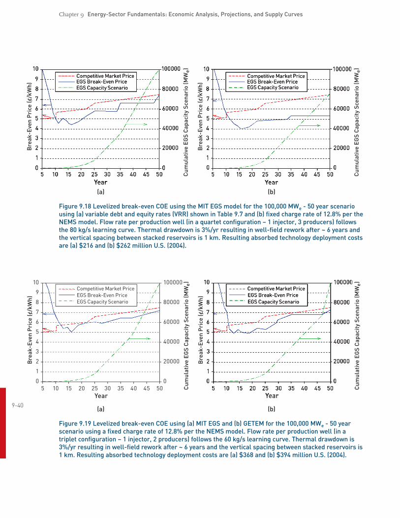
Chapter 9 EnergySector Fundamentals: Economic Analysis, Projections, and Supply Curves
(a) (b)
50
1
2
3
4
5
6
7
8
9
10
0
20000
40000
60000
80000
100000
10 15 20 25 30Year
35 40 45 50
Competitive Market PriceEGS Break-Even PriceEGS Capacity Scenario
Competitive Market PriceEGS Break-Even PriceEGS Capacity Scenario
50
1
2
3
4
5
6
7
8
9
10
0
20000
40000
60000
80000
100000
10 15 20 25 30Year
35 40 45 50
Bre
ak-E
ven
Pri
ce(c
/kW
h)
Bre
ak-E
ven
Pri
ce(c
/kW
h)
Cum
ulat
ive
EGS
Cap
acit
ySc
enar
io(M
W) e
Cum
ulat
ive
EGS
Cap
acit
ySc
enar
io(M
W) e
Figure 9.18 Levelized breakeven COE using the MIT EGS model for the 100,000 MWe 50 year scenario using (a) variable debt and equity rates (VRR) shown in Table 9.7 and (b) fixed charge rate of 12.8% per the NEMS model. Flow rate per production well (in a quartet configuration – 1 injector, 3 producers) follows the 80 kg/s learning curve. Thermal drawdown is 3%/yr resulting in wellfield rework after ~ 6 years and the vertical spacing between stacked reservoirs is 1 km. Resulting absorbed technology deployment costs are (a) $216 and (b) $262 million U.S. (2004).
50
1
2
3
4
5
6
7
8
9
10
0
20000
40000
60000
80000
100000
10 15 20 25 30Year
35 40 45 50
Competitive Market PriceEGS Break-Even PriceEGS Capacity Scenario
Competitive Market PriceEGS Break-Even PriceEGS Capacity Scenario
50
1
2
3
4
5
6
7
8
9
10
0
20000
40000
60000
80000
100000
10 15 20 25 30Year
35 40 45 50
Bre
ak-E
ven
Pri
ce(c
/kW
h)
Bre
ak-E
ven
Pri
ce(c
/kW
h)
Cum
ulat
ive
EGS
Cap
acit
ySc
enar
io(M
W) e
Cum
ulat
ive
EGS
Cap
acit
ySc
enar
io(M
W) e
940 (a) (b)
Figure 9.19 Levelized breakeven COE using (a) MIT EGS and (b) GETEM for the 100,000 MWe 50 year scenario using a fixed charge rate of 12.8% per the NEMS model. Flow rate per production well (in a triplet configuration – 1 injector, 2 producers) follows the 60 kg/s learning curve. Thermal drawdown is 3%/yr resulting in wellfield rework after ~ 6 years and the vertical spacing between stacked reservoirs is 1 km. Resulting absorbed technology deployment costs are (a) $368 and (b) $394 million U.S. (2004).

Chapter 9 EnergySector Fundamentals: Economic Analysis, Projections, and Supply Curves
9.12.3 Deriving cost and supply curves
Both the GETEM and MIT EGS model results suggest a favorable outcome from investments in EGS for baseload power. Figure 9.20 provides a demonstration of the impact of new applied technology and field learning. It demonstrates that as new phases of technology are developed and used in the field, the delivered cost of energy is forecast to fall below competitive baseload energy prices.
50
1
2
3
4
5
6
7
8
9
10
0
20000
40000
60000
80000
100000
10 15 20 25 30
Year35 40 45 50
Competitive Market PriceEGS Break-Even PriceEGS Capacity Scenario
Competitive Market PriceEGS Break-Even PriceEGS Capacity Scenario
50
1
2
3
4
5
6
7
8
9
10
0
20000
40000
60000
80000
100000
10 15 20 25 30
Year35 40 45 50
Bre
ak-E
ven
Pri
ce(c
/kW
h)
Bre
ak-E
ven
Pri
ce(c
/kW
h)
Cum
ulat
ive
EGS
Cap
acit
ySc
enar
io(M
W) e
Cum
ulat
ive
EGS
Cap
acit
ySc
enar
io(M
W) e
(a) (b)
Figure 9.20 Levelized breakeven COE using MIT EGS for the 100,000 MWe 50 year scenario using variable debt and equity rates (VRR) shown in Table 9.7. Flow rate per production well (in a quartet configuration – 1 injector, 3 producers) follows the 80 kg/s learning curve. Thermal drawdown is 3%/yr resulting in wellfield rework after ~ 6 years and the vertical spacing between stacked reservoirs are (a) 1 km and (b) 500m. Resulting absorbed technology deployment cost is $216 million U.S. (2004).
Figure 9.21 illustrates the effect of investments in EGS research and market adoption of new technology and drilling techniques. The figures show cumulative EGS capacity at 100,000 MWe, and assume flow rate per production well in quartet configuration of 80 kg/s with vertical spacing between stacked reservoirs is 1 km. Thermal drawdown is assumed to be 3%/year and wellfield rework and restimulation occurs approximately every six years.
In this scenario, variable debt and equity rates (VRR) are employed to gauge the impact on the breakeven price of EGS and the resultant cumulative supply additions while assuming the trend in competitive market price. The time period in which competitive prices can be achieved is estimated to be approximately 11 years after inception of significant efforts to expand research. Here the levelized energy cost (LEC), including forecast costs of redrilling and stimulation, approaches parity 941
with market prices. When viewed through the full 50year scenario, the analysis suggests that the competitive price of EGS remains below the price for other baseload power.
Continued expansion of facilities beyond that point will ultimately displace older coal and oilfired generation and forestall construction of other lesscompetitive baseload facilities including coal and nuclear power. This is apparent as cumulative additions to the supply curve extend it through the forecast period of 2050. During this period, beyond year 11, the market price of delivered EGS electricity is expected to be below competitive technologies.
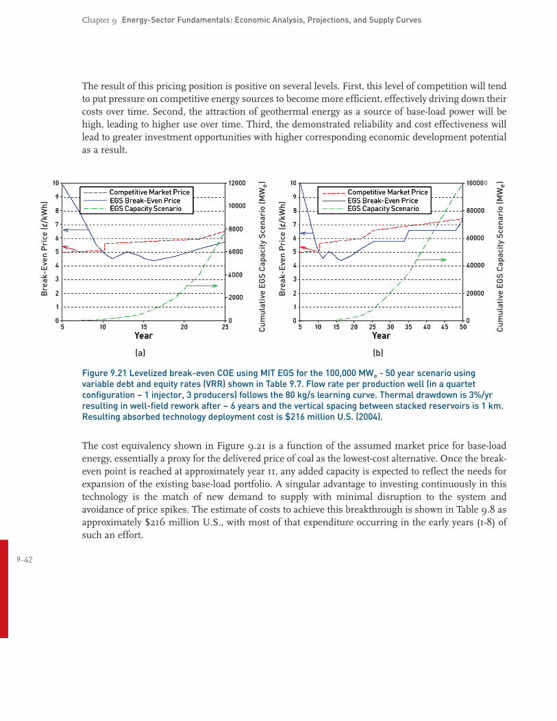
Chapter 9 EnergySector Fundamentals: Economic Analysis, Projections, and Supply Curves
The result of this pricing position is positive on several levels. First, this level of competition will tend to put pressure on competitive energy sources to become more efficient, effectively driving down their costs over time. Second, the attraction of geothermal energy as a source of baseload power will be high, leading to higher use over time. Third, the demonstrated reliability and cost effectiveness will lead to greater investment opportunities with higher corresponding economic development potential as a result.
50
1
2
3
4
5
6
7
8
9
10
0
2000
4000
6000
8000
10000
12000
10 15 20
Year25
Competitive Market PriceEGS Break-Even PriceEGS Capacity Scenario
Competitive Market PriceEGS Break-Even PriceEGS Capacity Scenario
50
1
2
3
4
5
6
7
8
9
10
0
20000
40000
60000
80000
100000
10 15 20 25 30
Year35 40 45 50
Bre
ak-E
ven
Pri
ce(c
/kW
h)
Bre
ak-E
ven
Pri
ce(c
/kW
h)
Cum
ulat
ive
EGS
Cap
acit
ySc
enar
io(M
W) e
Cum
ulat
ive
EGS
Cap
acit
ySc
enar
io(M
W) e
(a) (b)
Figure 9.21 Levelized breakeven COE using MIT EGS for the 100,000 MWe 50 year scenario using variable debt and equity rates (VRR) shown in Table 9.7. Flow rate per production well (in a quartet configuration – 1 injector, 3 producers) follows the 80 kg/s learning curve. Thermal drawdown is 3%/yr resulting in wellfield rework after ~ 6 years and the vertical spacing between stacked reservoirs is 1 km. Resulting absorbed technology deployment cost is $216 million U.S. (2004).
The cost equivalency shown in Figure 9.21 is a function of the assumed market price for baseload energy, essentially a proxy for the delivered price of coal as the lowestcost alternative. Once the breakeven point is reached at approximately year 11, any added capacity is expected to reflect the needs for expansion of the existing baseload portfolio. A singular advantage to investing continuously in this technology is the match of new demand to supply with minimal disruption to the system and avoidance of price spikes. The estimate of costs to achieve this breakthrough is shown in Table 9.8 as approximately $216 million U.S., with most of that expenditure occurring in the early years (18) of such an effort.
942

Chapter 9 EnergySector Fundamentals: Economic Analysis, Projections, and Supply Curves
Table 9.8 Relationship of year, output, cost and cost deficit – 80 kg/s learning curve, quartet configuration, 3% thermal drawdown, 1 km vertical reservoir spacing.
Year EGS EGS COE Baseload EGS deficit Total Cost Absorbed capacity (¢/kWh) market (¢/kWh) cost
(MWe) (¢/kWh)
5 25 9.99 5.00 4.99 $229,539,800 $114,612,500
7 60 7.82 5.06 2.77 $251,051,400 $88,766,000
9 120 5.56 5.11 0.45 $152,024,900 $12,401,900
10 180 4.92 5.65 0.00
11 240 4.52 5.67 0.00
13 400 5.06 5.72
14 550 4.75 5.77
15 750 4.53 5.78
16 1,000 4.40 5.82
19 2,000 4.69 5.89
22 4,000 5.24 5.98
25 8,000 5.78 6.58
34 30,982 5.74 6.86
35 35,000 6.59 6.91
48 92,778 6.58 7.38
50 100,000 7.43 7.45
Total $632,616,100 $215,780,400
The diffusion of technology scenario (100,000 MWe over 50 years) employed in this analysis is validated by Figure 9.21a and Table 9.8. Using the VRRbased MIT EGS model with the supply algorithm, we find a maximum cost differential at 35 years where EGS technology offers a premium source of energy for dispatch and has achieved sustained levels of capacity. Assuming a fiveyear lag period for permitting and construction, the point of maximum differential may occur more providently in year 40. The advantage (although, in reality, the supply of energy available is effectively infinite) lies in the fact that approximately 100,000 MWe are developed during the first phase of development. 943
9.13 ConclusionsWe have found a positive correlation between the development of new EGS fields and continued declines in delivered costs of energy. This finding reflects not only the economies from new techniques and access to higher value resources, but also the inevitable cost of competitive power sources. Analysis suggests that, with significant initial investment, installed capacity of EGS could reach 100,000 MWe within 50 years, with levelized energy costs at parity with market prices after 11
Chapter 9 EnergySector Fundamentals: Economic Analysis, Projections, and Supply Curves
years. It is projected that the total cost, including costs for research, development, demonstration, and deployment, required to reach this level of EGS generation capacity ranges from approximately $600 $900 million with an absorbed cost of $200$350 million.
In this period, we expect that the development of new EGS resources will occur at a critical time when grid stabilization with baseload power will be needed to avoid redirecting expensive natural gas facilities when they are most in demand worldwide.
EGS power lacks a demonstration of its capability at the present time. As pointed out in this report, this can be accomplished with a proven application of R&D support. We expect that the cost of power potential demonstrated in this chapter warrants a comprehensive research and demonstration effort to begin moving toward the period when replacement of retiring fossil and nuclear units and new capacity growth will most affect the U.S. electrical supply.
Footnotes1. A power transmission system is commonly referred to as a “grid.” However, for reasons of
economy, the network is rarely a grid (a fully connected network) in the mathematical sense. Redundant paths and lines are provided so that power can be routed from any power plant to any load center, through a variety of routes, based on the economics of the transmission path and the cost of power. Much analysis is done by transmission companies to determine the maximum reliable capacity of each line, which, due to system stability considerations, may be less than the physical limit of the line.
2. The revival of the FutureGen program at DOE underscores this trend.
3. In the IEO2005 reference case, coal continues to be the dominant fuel for generation of electricity and combined heat and power (district heat). In 2025, coal is projected to fuel 38% of the world’s electricity generation, compared with a 24% share for natural gas. Coalfired capacity is expected to grow by 1.5% per year, from 987 GWe in 2002 to 1,403 GWe in 2025. Installed coalfired capacity, as a share of total world capacity, declines from 30% to 26% over the forecast.
By country, the United States and China currently are the leaders in terms of installed coalfired capacity, at 311 and 204 GWe, respectively. In China, strong growth in naturalgasfired capacity is projected to push coal’s share down from 65% to 52% of total generating capacity. In the United States, coalfired power plants are expected to continue supplying most of the country’s electricity
944 through 2025. In 2002, coalfired plants in the United States (including utilities, independent power producers, and enduse combined heat and power) accounted for 51% of all electricity generation. While the output from U.S. coalfired power plants increases in the forecast, from 1,881 billion kWh in 2002 to 2,890 billion kWh in 2025, their share of total generation decreases slightly, to 50%, as a result of a rapid increase in naturalgasfired generation.
4. The source for declining transportation costs is not cited by the EIA.
5. According to the EIA, U.S. nuclear capacity is projected to increase from 99 GWe in 2002 to 103 GWe in 2025, in part because of the return of the Browns Ferry reactor, scheduled for 2007.
Chapter 9 EnergySector Fundamentals: Economic Analysis, Projections, and Supply Curves
6. For the mature market economies, the IEO (2005) reference case assumes that, in the long term, retirements of existing plants as they reach the end of their operating lives will not be balanced by the construction of new nuclear power capacity, and there will be a slight decline in installed nuclear capacity toward the end of the forecast.
7. Load firming is the acquisition of supply to fill a real or expected gap in guaranteed delivery of power to customers. Firm power is power or powerproducing capacity intended to be available at all times during the period covered by a guaranteed commitment to deliver, even under adverse conditions.
8. According to the EIA in 2004, retail sales of electricity increased to 3,548 billion kWh in 2004, a 1.7% increase from 2003 and a pace close to the historical growth rate. Revenue, however, increased to more than $270 billion in 2004, a 4.5% increase from 2003 and the second straight year of strong growth. All customer classes except transportation faced higher average retail prices in 2004, as the national average price across all sectors was 7.62 cents per kWh, up from 7.42 cents in 2003.
The average retail price in the residential sector increased to 8.97 ¢/kWh, a 3.1% increase from2003. In the commercial and industrial sectors, average price increases were 2.0% and 2.9%,respectively. Higher fossil fuel prices to electricity generators led to higher wholesale power costs.Average enduse prices increased dramatically in states where natural gas fuels significantportions of baseload generating capacity – Texas, Mississippi, Louisiana, and Florida.
9. For instance, in 2002, MidAmerica Energy dropped a project in the Salton Sea area of California, due to constraints on transmission access and capacity, (M. Masri, chief of Renewable Programs, California Energy Commission, personal communication).
10. Power is defined as the rate of flow of energy past a given point. In “alternating current” circuits, energy storage elements such as inductance and capacitance may result in periodic reversals of the direction of energy flow. The portion of power flow that, averaged over a complete cycle of the AC waveform, results in net transfer of energy in one direction is known as real power. That portion of power flow due to stored energy, which returns to the source in each cycle, is known as reactive power.
11. Direct current (DC or “continuous current”) is the continuous flow of electric charge through a conductor such as a wire from high to low potential.
12. See California Energy Commission emergency siting process for 2000. 945
13. The energy attribute may be considered as a separate value, which is not purchased directly but which may be priced, such as renewable attributes, reliability, “cleanness,” etc.
14. Reactive energy (VARs) is defined as the imaginary component of the vector product of the voltage and current, each expressed as a vector and used to provide line stability.
15. Each surface complex is assumed to be composed of power turbines nominally rated at 60 MWe, and combined in modules dependent on the resource being accessed.

Chapter 9 EnergySector Fundamentals: Economic Analysis, Projections, and Supply Curves
16. Supply curves for EGS power in selected specific states are given in Appendix A.9.4. An example of a state in an area with no operating hydrothermal geothermal plants is Texas, shown in Figure A.9.15. Hightemperature gradients in the Gulf Coast area have been discovered during drilling for oil and gas. The hot water coproduced with oil and gas production is discussed in Chapters 2 and 7. The EGS resource base for these fluids could also be developed on its own. While the costs for developing geothermal resources in Texas are currently higher than market, the amount of power available is significant and, with incremental improvements in cost, could represent a significant baseload resource. Colorado (Figure A.9.16) is a state with both identified hydrothermal resources and identified EGS resources at depths shallower than 3 km – there is also a significant EGS resource at depths greater than 3 km. About 42 GWe could be available by 2011 at a cost of less than 10¢/kWh based on the continued success of the Soultz project or other EGS field projects if drilling cost improvements and conversion technology improvements continue to be made.
17. For a normal distribution, 95.45% of the area is within two standard deviations. Therefore, after more than two standard deviations on both sides of the distribution (40 years), about 95% of the EGS capacity would be installed.
18. The technologies described in this paper are an extension of existing geothermal drilling and fracturing techniques, only to the extent that drilling and fracturing are taking place at depth. The techniques are assumed to be more precise and capable of delivering higher rates of power over longer periods of time than previous hydrothermal systems. Thus, although these systems may be collocated in existing geothermal fields, the depth and accessed heat resource are beyond current established technology and power conversion.
19. A 2% area utilization is a conservative estimate of potential resources at depth. We have chosen this level to find coincident breakeven points for the cost of capital, which is assumed to be borne by the private sector after the initial 6,000 MWe.
946
Chapter 9 EnergySector Fundamentals: Economic Analysis, Projections, and Supply Curves
ReferencesAnderson, B.J. 2006. Personal communication, West Virginia University, Department of ChemicalEngineering, Morgantown, W.V.
Armstead, H. C. H. and J. W. Tester. 1987. Heat mining: a new source of energy. E. & F.N. Spon, London.
Brett, J. F. and K. K. Millheim. 1986. “The Drilling Performance Curve: A Yardstick for JudgingDrilling Performance SPE 15362.” SPE Annual Technical Conference and Exhibition, October 58, NewOrleans, Louisiana.
CEC. 2006. California Energy Commission Web site. Accessed March 9, 2006.http://energy.ca.gov/geothermal/index.html
DOE. 1997. “Renewable Energy Technology Characterizations.” TR109496. EERE Office of UtilityTechnologies, U.S. Department of Energy.
EIA. 2002. “Inventory of Electric Utility Power Plants in the United States 2000.” EnergyInformation Administration, U.S. Department of Energy.
EIA. 2004. “Annual Electric Power Industry Report.” Form EIA861, Energy InformationAdministration, U.S. Department of Energy.
EIA. 2005. “Annual Energy Outlook 2005: Electricity Supply.” AEO2005. Energy InformationAdministration, U.S. Department of Energy.
GEA. 2006. Figures released by Geothermal Energy Association, Washington, DC.
Herzog, H. J., J. W. Tester, et al. 1997. “Economic analysis of heat mining.” Energy Sources, 19(1): 1933.
Ikoku, C. U. 1978. “Application of Learning Curve Models to Oil and Gas Well Drilling SPE 7119.”SPE California Regional Meeting, April 1214, San Francisco, California.
Kravis, S., R. Irrgang, et al. 2004. “The Trouble Probability Plot: A New Measure of Drilling Maturity SPE 89959.” SPE Annual Technical Conference and Exhibition, September 2629, Houston, Texas.
MacGregor, P. R., C. E. Maslak, et al. 1991. “The Market Outlook for Integrated GasificationCombined Cycle Technology.” New York, General Electric Company.
McDonald, A. and L. Schrattenholzer. 2001. “Learning rates for energy technologies.” Energy Policy, 29(4): 255261.
Moore, M.C. and D.J. Arent, 2006. “R&D Advancement, Technology Diffusion, and the Impact onEvaluation of Public R&D,” Energy Policy. 947
Muffler, L. J. P. and M. Guffanti (eds.), 1979. “Assessment of geothermal resources in the UnitedStates – 1978.” US Geol. Surv. Circ. 790.
Nakicenovi´c, N., A. Grübler, et al. 1998. Global energy perspectives. Cambridge University Press, Cambridge, New York.
Petty, S., B. J. Livesay, and W. P. Long. 1991. “Supply of Geothermal Power from Hydrothermal Sources.” Contractor Report, Sandia National Laboratory.
Petty, S. and G. Porro. 2006. Personal communications.

Chapter 9 EnergySector Fundamentals: Economic Analysis, Projections, and Supply Curves
Renner, J. L., D. E. White, and D. L. Williams. 1975. “Hydrothermal Convection Systems,” in White, D. E. and D. L. Williams, (Eds.), Assessment of Geothermal Resources of the United States – 1975. US Geol. Surv. Circ. 726.
Rogers, E. M. 2003. Diffusion of innovations. New York, Free Press.
Stoft, S. 2002. Power System Economics: Designing Markets for Electricity. IEEE Press.
Tester, J. W., H. J. Herzog, et al. 1990. “Economic predictions for heat mining: a review and analysis of hot dry rock (HDR) geothermal energy technology.” Energy Laboratory, Massachusetts Institute of Technology, Cambridge, Mass.
Tester, J. W. and H. J. Herzog. 1991. “The Economics of Heat Mining: An Analysis of Design Options and Performance Requirements of Hot Dry Rock (HDR) Geothermal Power Systems.” Sixteenth Workshop on Geothermal Reservoir Engineering, January 2325, Stanford University, Stanford, California.
948

Chapter 9 EnergySector Fundamentals: Economic Analysis, Projections, and Supply Curves
AppendicesA.9.1 Baseload Power in Grid Operations
Baseload plants tend to be older than gasfired combustion turbine units and are usually powered by coal, oil, or nuclear fuel – they also can be hydroelectric. In contrast, most peakload plants, called “peaking units,” are fueled by natural gas. Intermediateload – or midrange loadfollowing plants – are often smaller, older, coalfueled plants that have been modified to allow them to ramp up and down without damage.
As system loads have grown, new generation has been built to supply that load. However, there have been relatively few new baseload plants completed in the United States since the 1990s. Thus, the baseload units tend to be older than the gasfired combustion turbine units and are usually powered by nuclear, coal, and, to a very small extent, oil. The new plants have either been of the midrange loadfollowing or peak varieties. Peaking plants may only run for 100 to 200 hours a year and, at most, a few hours in any given day. Midrange loadfollowing plants may serve load in key daytime hours by following load changes during the day.
Therefore, there has been a small and gradual shift in the percentage of the system load served from baseload plants to midrange plants. The amount of load served by peaking plants grew somewhat during the 1990s, but has leveled off during the past decade. Natural gasfired plants, originally deployed for peaking capacity, are now increasingly being used for baseload power. This has tended to increase prices of delivered energy in many urban markets in the United States. Furthermore, the dramatic increase in the price of natural gas has resulted in many stranded combinedcycle units, unable to produce economical electricity in the current market.
As a result of some older power plants being taken out of service and because of the types of new plants that have been built, the amount of natural gasfueled generation to serve overall load has increased. At the same time, the amount of generation fueled by coal has remained relatively constant.
During the past decade, a move to install new gasfired combinedcycle plants has displaced some of the new demand for coal power generation. This phenomenon seems to be abating in the face of sustained and expected high prices for natural gas in domestic, Canadian, and imported markets. As a consequence, future use of natural gas for baseload power generation is likely to be constrained by price and, ultimately, by supply. Simultaneously, expansion of coalbased power generation is constrained by environmental and air quality regulations that have slowed new permitting and suggest stricter plant design criteria in the future.2
949The baseload requirements of most regions are served by a combination of coalfired generation, nuclear steam generation, and hydroelectric facilities. There are several features of this combination of resources that suggest higher prices and tightened supplies in the future. These include: a. fuel prices b. additions of new generating capacity and capacity constraints c. transmission capacity d. retirements of existing stock e. environmental regulations and future CO2 emissions costs.

Chapter 9 EnergySector Fundamentals: Economic Analysis, Projections, and Supply Curves
A.9.1.1 Coalfired generation in base load
Coal prices have been climbing at a rate of approximately 0.5% per year (without indexing for inflation) for the past decade, although not consistently yeartoyear. Some of this increase reflects the preference for lowsulphur coal available from the Powder River Basin, which entails higher demand on an already constrained railroad capacity resulting in higher transportation costs. Also, simple supply/demand balances show steady pressure on existing sources. A lack of new transmission capacity, a limited ability to expand existing coal facilities near urban areas, and compliance with tighter environmental standards makes delivered power slightly more expensive. In addition, retirement of existing facility stock, which was largely constructed in the mid1900s and is less efficient than modern units, has contributed to the increase in overall costs. Finally, the demand for coal used in metallurgical operations (such as coking) is in competition for coal demanded for energy generation; this may be exacerbated when newer coal gasification and liquefaction facilities become more economical to construct in the future.3
Coal plays an important and, in some regions, dominant role in baseload power delivery. Coal consumption in the United States as a share of fuels used for electricity generation is expected to increase from 52% to 53% over the forecast. In terms of installed capacity, coal’s share of the total will hold steady at 35%. Coal is used for baseload generation, which explains why it accounts for only 35% of U.S. capacity but generates more than onehalf of the country’s electricity. In Figure A.9.1, the significance of that role is graphically illustrated.
950
United States Total = 1,015.1 (1.0%)Pacific
Contiguous9.9 (-7.8%)
WestNorth Central146.7 (-0.8%)
Mountain118.5 (1.6%)
EastNorth Central229.0 (2.1%)
West South Central152.9 (0.8%)
PacificNoncontiguous
1.4 (21.8%)
New England8.3 (1.8%)
Middle Atlantic67.5 (4.3%)
South Atlantic170.9 (-0.6%)
EastSouth Central109.0 (2.0%)
Figure A.9.1 Electric powersector consumption of coal by Census region, 2004 (million short tons and percent change from 2003) (EIA, 2005).
According to the EIA, to a large extent, the projections of increasing prices for natural gas after 2010 – combined with projections of relatively stable coal prices and slightly declining rates for domestic transportation of coal4 – have been the key factors helping coal compete as a fuel for U.S. power generation. Increases in coalfired generation are projected to result from both greater utilization of

Chapter 9 EnergySector Fundamentals: Economic Analysis, Projections, and Supply Curves
existing U.S. coalfired generating capacity and an additional 89,500 MWe of new coalfired capacity by 2025 (3,600 MWe of older coalfired capacity is projected to be retired). The average utilization rate of coalfired generating capacity is projected to increase from 70% in 2002 to 83% in 2025. A coalfired plant produces the lowestcost electricity when gas prices are higher than $2.80 per million (MMBtu).
A.9.1.2 Nuclear steam generation
The price of nuclearsourced electricity has remained relatively constant during the past decade, a reflection of better management and ongoing maintenance of facilities compared to earlier periods. Spent fuel continues to be stored onsite in most facilities and could be a source of longterm price increases in the future as spent fuel becomes increasingly difficult to manage onsite. Although there are new facilities in design, no recent construction has taken place in the United States, which would augment the existing stock of nuclear facilities. The earliest, currently operating commercial nuclear facilities were constructed in 19691970, with a large fraction of the generation base constructed in the 1980s. Assuming the design life of a nuclear plant is 25 years, with regulatory extensions available to 40 years before retirement, 46 GWe of capacity can be expected to retire in the period to 2020.5
This represents about 46% of the nearly 99 GWe of current baseload power from this source. Environmental regulations, public concerns over safety, uncertainty over the storage of spent fuel, and investor concerns over financial risk combine to make expansion and replacement of this source of power problematic. Assuming 50% of the retired stock is replaced during the next 15 years, the resulting gap in baseload capacity could approach 25 GWe.
6
A.9.1.3 Hydroelectric facilities
Hydroelectric facilities continue to provide a critical backbone of the baseload capacity for U.S. power networks in areas served by the Western Area Power Administration (WAPA) or the Bonneville Power Administration (BPA). A proven technology, hydroelectric plants are dispatchable efficiently for both baseload and load firming,7 and are the core of operations for federal agencies such as BPA and WAPA, underpinning the transmission facilities built to transmit power from the large hydroelectric project areas. Increased environmental concerns over the use of water, reduced capacity due to siltation, and changes in rainfall patterns have created some uncertainty in the availability of this power source. Because no new hydroelectric facilities are planned or are likely in the next decade, this source of power should be considered static or in slight decline.
A.9.1.4 Baseload power prices and electricity supply sources
Prices for baseload power do not generally change rapidly, due, in part, to the fact that most are controlled through longterm contracts. Given all the factors cited above, however, we expect the 951 competitive price for baseload power bid into system operations to increase from about 45 cents/kWh to 67 cents/kWh during the next 10 years.8 Figure A.9.2 shows the price of electricity on a statebystate basis across the United States.

Chapter 9 EnergySector Fundamentals: Economic Analysis, Projections, and Supply Curves
i
United States Total Average Price per kilowatthour is 7.62 Cents
Average Price(Cents per kilowatthour)
4.63 to 5.80
6.07 to 6.43
6.44 to 7.00
7.10 to 9.69
10.26 to 15.70
VT
11.02 11.37
NH
ME9.69
10.77
10.96
10.26
10.29
MA
RI
CT
NJDE
MD
DC 7.47
7.15
7.53
12.55
8.006.89
6.94
5.586.80
6.88
4.61
6.14
NY
PA
VAWV
OH
MIWI
INIL
IA
TN
SCGA
FL
ALMS
LATX
AK
CA
NV
IDOR
WA
HI10.99
15.70
OK
KS
NE
SD
NDMNMT
WY
CO
NMAZ
UT
6.50
6.37
5.70
6.44
5.696.246.40
4.984.976.21
5.80
6.955.698.56
7.107.45
11.45AR
MO
8.16
6.586.087.00
7.137.95
5.67
6.07
6.40
6.22
KY
NC6.97
6.435.13
Note: Figure information is shown by 5 groupings of 10 States and The District of Columbia. The presented range moves from the values for the lowest 10 States to the top 10 States.Source: Energy Information Administration, Form EIA-861, “Annual Electric Power Industry Report.”
Figure A.9.2 Average reta l electricity price by state, 2004 (in ¢/kWh or cents per kilowatt hour) (EIA, 2004).
A look at the U.S. electricity generation base (see Table A.9.1) shows that the available power supplies are increasing, but are offset by planned retirements of existing facilities reflecting a high concentration of use for baseload operations.
We have summed the highestcapacity energy generating sources in Figure A.9.3. It shows the disproportionate share borne by fossil facilities in the current energy mix.
DOE had estimated (see Table A.9.2) that there would be significant additions to the existing generating stock during 20012005, based on anticipated applications for new siting licenses. The list is notable for the absence of any new nuclear or hydroelectric facilities.
952 During this same period, the grid in the United States experienced significant retirement of existing capacity, mainly in older petroleum (oil)fired generation and simplecycle gas turbines (see Table A.9.3). The DOE has suggested that there will be a significant amount of new generation sited in coming decades as shown in Figure A.9.4, relative to expected retirements. Our projections of nuclear plant retirements, as well as older coal facilities, would cause this projection to increase slightly during 20212030.

Chapter 9 EnergySector Fundamentals: Economic Analysis, Projections, and Supply Curves
Table A.9.1 Existing U.S. generation base (EIA, 2005; and GEA, 2006).
Existing No. Generator Net Summer Net Winter
of Units Nameplate MWe MWe MWe
U.S. Total 16,770 1,049,615 962,942 999,749
Geothermal 212 3,119 2,170 2,311
Coal 1,526 335,243 313,020 315,364
Petroleum 3,175 37,970 33,702 37,339
Natural Gas 3,048 256,627 224,257 241,391
Dualfired 3,003 193,115 172,170 184,399
Other Gases 119 2,535 2,296 2,259
Nuclear 104 105,560 99,628 101,377
Hydroelectric Conventional 3,995 77,130 77,641 77,227
Pumped Storage 150 19,569 20,764 20,676
Wind 246 6,552 6,456 6,456
Wood/Wood Waste 171 2,864 2,583 2,582
Municipal Solid Waste 98 2,677 2,196 2,217
Biomass gas 90 243 200 232
Solar (photovoltaic, thermal) 17 404 398 366
Landfill gas 582 934 859 879
Agricultural byproduct 26 289 274 268
Black liquor (biomass) Not available ~ 4,000 ~ 4,000 ~ 4,000
Other 42 754 700 716
953
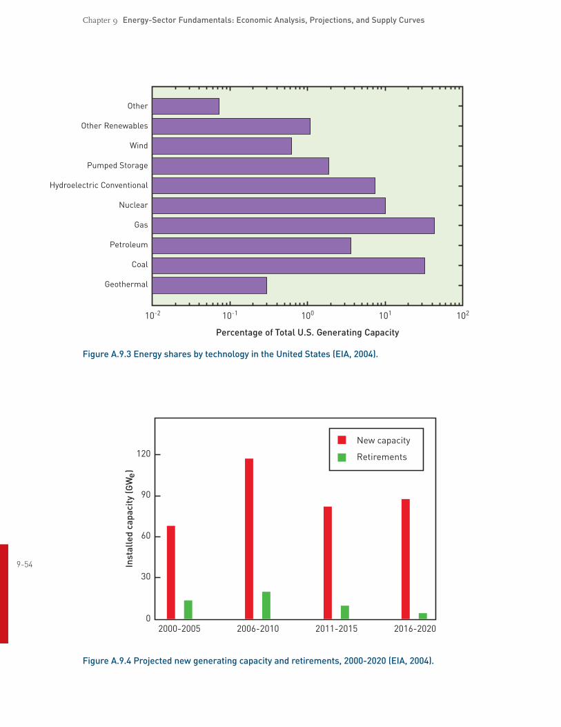
Chapter 9 EnergySector Fundamentals: Economic Analysis, Projections, and Supply Curves
Geothermal
Coal
Petroleum
Gas
Nuclear
Hydroelectric Conventional
Pumped Storage
Wind
Other Renewables
Other
10-2 10-1 100 101 102
Percentage of Total U.S. Generating Capacity
Figure A.9.3 Energy shares by technology in the United States (EIA, 2004).
954 Inst
alle
dca
paci
ty(G
W)
2016-20200
120
30
60
90
2000-2005 2006-2010 2011-2015
New capacity
Retirements
e
Figure A.9.4 Projected new generating capacity and retirements, 20002020 (EIA, 2004).
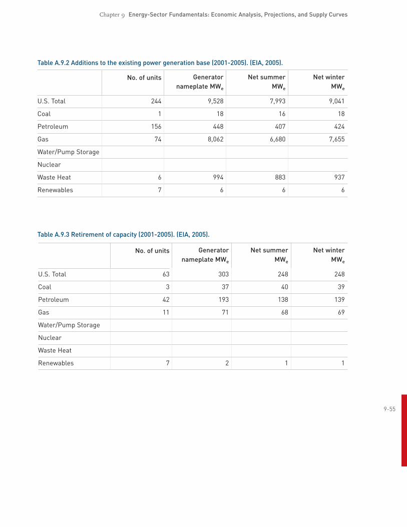
Chapter 9 EnergySector Fundamentals: Economic Analysis, Projections, and Supply Curves
Table A.9.2 Additions to the existing power generation base (20012005). (EIA, 2005).
No. of units Generator Net summer Net winter nameplate MWe MWe MWe
U.S. Total 244 9,528 7,993 9,041
Coal 1 18 16 18
Petroleum 156 448 407 424
Gas 74 8,062 6,680 7,655
Water/Pump Storage
Nuclear
Waste Heat 6 994 883 937
Renewables 7 6 6 6
Table A.9.3 Retirement of capacity (20012005). (EIA, 2005).
Generator Net summer Net winter No. of units nameplate MWe MWe MWe
63 303 248 248
Coal 3 37 40 39
42 193 138 139
Gas 11 71 68 69
7 2 1 1
U.S. Total
Petroleum
Water/Pump Storage
Nuclear
Waste Heat
Renewables
955
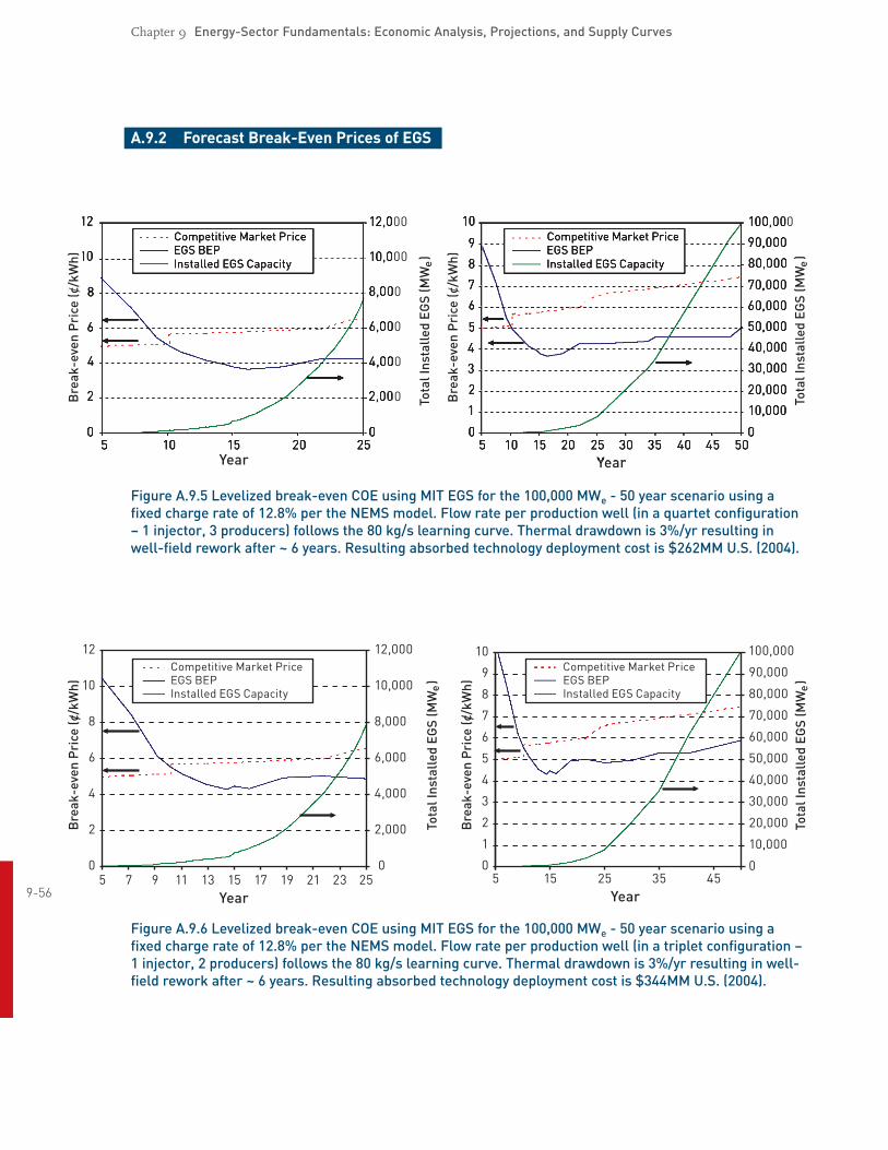
5 7 9 11 13 15 17 19 21 230
2
4
6
8
12
10
0
2,000
4,000
6,000
8,000
10,000
12,000
Year25
Competitive Market PriceEGS BEPInstalled EGS Capacity
Competitive Market PriceEGS BEPInstalled EGS Capacity
50
1
2
3
4
5
6
7
8
9
10
0
20,000
40,000
60,000
80,000
100,000
10,000
30,000
50,000
70,000
90,000
15 25Year
35 45
Bre
ak-e
ven
Pri
ce(c
/kW
h)
Bre
ak-e
ven
Pri
ce(c
/kW
h)
Tota
lIns
talle
dEG
S(M
W)
e
Tota
lIns
talle
dEG
S(M
W)
e
Chapter 9 EnergySector Fundamentals: Economic Analysis, Projections, and Supply Curves
A.9.2 Forecast BreakEven Prices of EGS
50
2
4
6
8
12
10
0
2,000
4,000
6,000
8,000
10,000
12,000
10 15 20Year
25
Competitive Market PriceEGS BEPInstalled EGS Capacity
Bre
ak-e
ven
Pri
ce(c
/kW
h)
Bre
ak-e
ven
Pri
ce(c
/kW
h)5
0
1
2
3
4
5
6
7
8
9
10Competitive Market PriceEGS BEPInstalled EGS Capacity
0
20,000
40,000
60,000
80,000
100,000
10,000
30,000
50,000
70,000
90,000
10 15 20 25 30Year
35 40 45 50
Tota
lIns
talle
dEG
S(M
W)
e
Tota
lIns
talle
dEG
S(M
W)
e
Figure A.9.5 Levelized breakeven COE using MIT EGS for the 100,000 MWe 50 year scenario using a fixed charge rate of 12.8% per the NEMS model. Flow rate per production well (in a quartet configuration – 1 injector, 3 producers) follows the 80 kg/s learning curve. Thermal drawdown is 3%/yr resulting in wellfield rework after ~ 6 years. Resulting absorbed technology deployment cost is $262MM U.S. (2004).
956
Figure A.9.6 Levelized breakeven COE using MIT EGS for the 100,000 MWe 50 year scenario using a fixed charge rate of 12.8% per the NEMS model. Flow rate per production well (in a triplet configuration – 1 injector, 2 producers) follows the 80 kg/s learning curve. Thermal drawdown is 3%/yr resulting in wellfield rework after ~ 6 years. Resulting absorbed technology deployment cost is $344MM U.S. (2004).
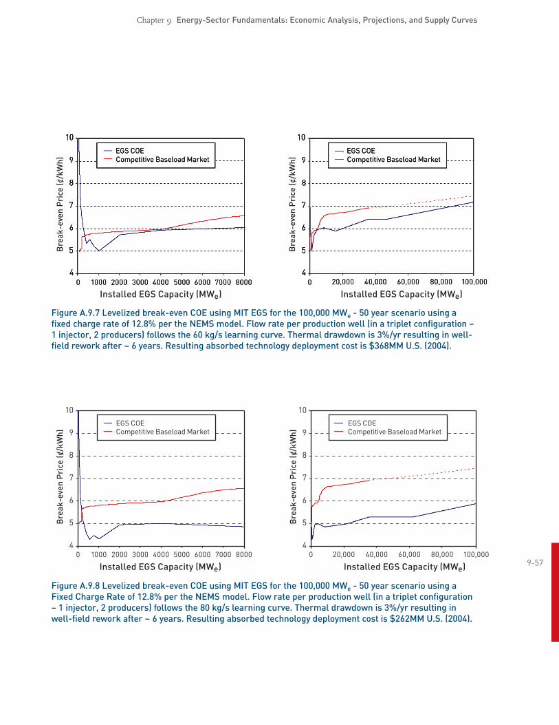
Chapter 9 EnergySector Fundamentals: Economic Analysis, Projections, and Supply Curves
0 1000 2000 3000 4000 5000 6000 70004
5
6
7
8
10
9
8000
EGS COECompetitive Baseload Market
0 20,000 40,000 60,000 80,0004
5
6
7
8
10
9
100,000
EGS COECompetitive Baseload Market
Bre
ak-e
ven
Pri
ce(c
/kW
h)
Bre
ak-e
ven
Pri
ce(c
/kW
h)Installed EGS Capacity (MW )e Installed EGS Capacity (MW )e
Figure A.9.7 Levelized breakeven COE using MIT EGS for the 100,000 MWe 50 year scenario using a fixed charge rate of 12.8% per the NEMS model. Flow rate per production well (in a triplet configuration – 1 injector, 2 producers) follows the 60 kg/s learning curve. Thermal drawdown is 3%/yr resulting in wellfield rework after ~ 6 years. Resulting absorbed technology deployment cost is $368MM U.S. (2004).
957 0 1000 2000 3000 4000 5000 6000 7000
4
5
6
7
8
10
9
8000
EGS COECompetitive Baseload Market
0 20,000 40,000 60,000 80,0004
5
6
7
8
10
9
100,000
EGS COECompetitive Baseload Market
Bre
ak-e
ven
Pri
ce(c
/kW
h)
Bre
ak-e
ven
Pri
ce(c
/kW
h)
Installed EGS Capacity (MW )e Installed EGS Capacity (MW )e
Figure A.9.8 Levelized breakeven COE using MIT EGS for the 100,000 MWe 50 year scenario using a Fixed Charge Rate of 12.8% per the NEMS model. Flow rate per production well (in a triplet configuration – 1 injector, 2 producers) follows the 80 kg/s learning curve. Thermal drawdown is 3%/yr resulting in wellfield rework after ~ 6 years. Resulting absorbed technology deployment cost is $262MM U.S. (2004).

Chapter 9 EnergySector Fundamentals: Economic Analysis, Projections, and Supply Curves
A.9.3 Cost Sensitivities
Clear Lake
(a) 40 kg/s production well flow rate (b) 20 kg/s production well flow rate
% Change From Base Case-60
7
8
9
10
-40 -20 0 20 40 606
Thermal Drawdown RateBond Debt Interest RateEquity Rate of Return% Bond vs Equity Debt
Drilling & Completion CostStimulation CostSurface Plant Capital CostFlow Rate/Production Well
Leve
lized
Cos
tofE
lect
rici
ty(c
/kW
h)
% Change From Base Case-60
9
10
12
14
-40 -20 0 20 40 60
11
13
8
Thermal Drawdown RateBond Debt Interest RateEquity Rate of Return% Bond vs Equity Debt
Drilling & Completion CostStimulation CostSurface Plant Capital CostFlow Rate/Production Well
Leve
lized
Cos
tofE
lect
rici
ty(c
/kW
h)
(c) Mature technology: 80 kg/s production well flow rate, quartet configuration
958 % Change From Base Case-60
3.0
3.5
4.0
4.5
-40 -20 0 20 40 60
Thermal Drawdown RateBond Debt Interest RateEquity Rate of Return% Bond vs Equity Debt
Drilling & Completion CostStimulation CostSurface Plant Capital CostFlow Rate/Production Well
Leve
lized
Cos
tofE
lect
rici
ty(c
/kW
h)
Figure A.9.9 Sensitivity of base case EGS LEC for the Clear Lake (Kelseyville, Calif.) scenario, showing levelized cost of electricity in ¢/kWh for three different production well flow rates.

Chapter 9 EnergySector Fundamentals: Economic Analysis, Projections, and Supply Curves
Conway
(a) 40 kg/s production well flow rate (b) 20 kg/s production well flow rate
% Change From Base Case-60
35
40
50
60
-40 -20 0 20 40 60
45
55
30
Thermal Drawdown RateBond Debt Interest RateEquity Rate of Return% Bond vs Equity Debt
Drilling & Completion CostStimulation CostSurface Plant Capital CostFlow Rate/Production Well
Leve
lized
Cos
tofE
lect
rici
ty(c
/kW
h)
% Change From Base Case-60 -40 -20 0 20 40 60
50
55
60
65
70
75
80
85
Thermal Drawdown RateBond Debt Interest RateEquity Rate of Return% Bond vs Equity Debt
Drilling & Completion CostStimulation CostSurface Plant Capital CostFlow Rate/Production Well
Leve
lized
Cos
tofE
lect
rici
ty(c
/kW
h)
(c) Mature technology: 80 kg/s production well flow rate, quartet configuration
959 % Change From Base Case
-60
11
-40 -20 0 20 40 606
7
8
9
10
Thermal Drawdown RateBond Debt Interest RateEquity Rate of Return% Bond vs Equity Debt
Drilling & Completion CostStimulation CostSurface Plant Capital CostFlow Rate/Production Well
Leve
lized
Cos
tofE
lect
rici
ty(c
/kW
h)
Figure A.9.10 Sensitivity of base case EGS LEC for the Conway, N.H., scenario, showing levelized cost of electricity in ¢/kWh for three different production well flow rates.

Chapter 9 EnergySector Fundamentals: Economic Analysis, Projections, and Supply Curves
Winnie, Texas, in the East Texas Basin
(a) 40 kg/s production well flow rate (b) 20 kg/s production well flow rate
% Change From Base Case-60
17
19
23
27
-40 -20 0 20 40 60
21
25
15
Thermal Drawdown RateBond Debt Interest RateEquity Rate of Return% Bond vs Equity Debt
Drilling & Completion CostStimulation CostSurface Plant Capital CostFlow Rate/Production Well
Leve
lized
Cos
tofE
lect
rici
ty(c
/kW
h)
% Change From Base Case-60 -40 -20 0 20 40 60
22
24
26
28
30
32
34
36
38
Thermal Drawdown RateBond Debt Interest RateEquity Rate of Return% Bond vs Equity Debt
Drilling & Completion CostStimulation CostSurface Plant Capital CostFlow Rate/Production Well
Leve
lized
Cos
tofE
lect
rici
ty(c
/kW
h)
(c) Mature technology: 80 kg/s production well flow rate, quartet configuration
960
% Change From Base Case-60
5.0
5.5
6.5
7.5
-40 -20 0 20 40 60
6.0
7.0
4.5
Thermal Drawdown RateBond Debt Interest RateEquity Rate of Return% Bond vs Equity Debt
Drilling & Completion CostStimulation CostSurface Plant Capital CostFlow Rate/Production Well
Leve
lized
Cos
tofE
lect
rici
ty(c
/kW
h)
Figure A.9.11 Sensitivity of base case EGS LEC for the East Texas Basin (Winnie, Texas) scenario, showing levelized cost of electricity in ¢/kWh for three different production well flow rates.
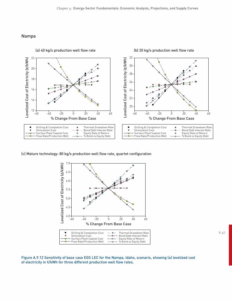
Chapter 9 EnergySector Fundamentals: Economic Analysis, Projections, and Supply Curves
Nampa
(a) 40 kg/s production well flow rate (b) 20 kg/s production well flow rate
% Change From Base Case-60 -40 -20 0 20 40 60
12
14
16
18
20
22
Thermal Drawdown RateBond Debt Interest RateEquity Rate of Return% Bond vs Equity Debt
Drilling & Completion CostStimulation CostSurface Plant Capital CostFlow Rate/Production Well
Leve
lized
Cos
tofE
lect
rici
ty(c
/kW
h)
% Change From Base Case-60 -40 -20 0 20 40 60
20
22
24
26
28
30
32
Thermal Drawdown RateBond Debt Interest RateEquity Rate of Return% Bond vs Equity Debt
Drilling & Completion CostStimulation CostSurface Plant Capital CostFlow Rate/Production Well
Leve
lized
Cos
tofE
lect
rici
ty(c
/kW
h)
(c) Mature technology: 80 kg/s production well flow rate, quartet configuration
961
% Change From Base Case-60
4.5
5.0
6.0
7.0
-40 -20 0 20 40 60
5.5
6.5
4.0
Thermal Drawdown RateBond Debt Interest RateEquity Rate of Return% Bond vs Equity Debt
Drilling & Completion CostStimulation CostSurface Plant Capital CostFlow Rate/Production Well
Leve
lized
Cos
tofE
lect
rici
ty(c
/kW
h)
Figure A.9.12 Sensitivity of base case EGS LEC for the Nampa, Idaho, scenario, showing (a) levelized cost of electricity in ¢/kWh for three different production well flow rates.

Chapter 9 EnergySector Fundamentals: Economic Analysis, Projections, and Supply Curves
Sisters
(a) 40 kg/s production well flow rate (b) 20 kg/s production well flow rate
% Change From Base Case-60 -40 -20 0 20 40 60
9
10
11
12
13
14
15
16
Thermal Drawdown RateBond Debt Interest RateEquity Rate of Return% Bond vs Equity Debt
Drilling & Completion CostStimulation CostSurface Plant Capital CostFlow Rate/Production Well
Leve
lized
Cos
tofE
lect
rici
ty(c
/kW
h)
% Change From Base Case-60 -40 -20 0 20 40 60
14
16
18
20
22
Thermal Drawdown RateBond Debt Interest RateEquity Rate of Return% Bond vs Equity Debt
Drilling & Completion CostStimulation CostSurface Plant Capital CostFlow Rate/Production Well
Leve
lized
Cos
tofE
lect
rici
ty(c
/kW
h)
(c) Mature technology: 80 kg/s production well flow rate, quartet configuration
962
% Change From Base Case-60 -40 -20 0 20 40 60
3.5
4.0
4.5
5.0
5.5
6.0
Thermal Drawdown RateBond Debt Interest RateEquity Rate of Return% Bond vs Equity Debt
Drilling & Completion CostStimulation CostSurface Plant Capital CostFlow Rate/Production Well
Leve
lized
Cos
tofE
lect
rici
ty(c
/kW
h)
Figure A.9.13 Sensitivity of base case EGS LEC for the Sisters, Ore., scenario showing levelized cost of electricity in ¢/kWh for three different production well flow rates.

Chapter 9 EnergySector Fundamentals: Economic Analysis, Projections, and Supply Curves
Poplar Dome
(a) 40kg/s production well flow rate (b) 20 kg/s production well flow rate
% Change From Base Case-60 -40 -20 0 20 40 60
11
12
13
14
15
16
17
18
Thermal Drawdown RateBond Debt Interest RateEquity Rate of Return% Bond vs Equity Debt
Drilling & Completion CostStimulation CostSurface Plant Capital CostFlow Rate/Production Well
Leve
lized
Cos
tofE
lect
rici
ty(c
/kW
h)
% Change From Base Case-60 -40 -20 0 20 40 60
17
19
21
23
25
Thermal Drawdown RateBond Debt Interest RateEquity Rate of Return% Bond vs Equity Debt
Drilling & Completion CostStimulation CostSurface Plant Capital CostFlow Rate/Production Well
Leve
lized
Cos
tofE
lect
rici
ty(c
/kW
h)
(c) Mature technology: 80 kg/s production well flow rate, quartet configuration
963
% Change From Base Case-60
4.5
5.0
6.0
7.0
-40 -20 0 20 40 60
5.5
6.5
4.0
Thermal Drawdown RateBond Debt Interest RateEquity Rate of Return% Bond vs Equity Debt
Drilling & Completion CostStimulation CostSurface Plant Capital CostFlow Rate/Production Well
Leve
lized
Cos
tofE
lect
rici
ty(c
/kW
h)
Figure A.9.14 Sensitivity of base case EGS LEC for the Poplar Dome (Poplar, Mont.) scenario, showing levelized cost of electricity in ¢/kWh for three different production well flow rates.
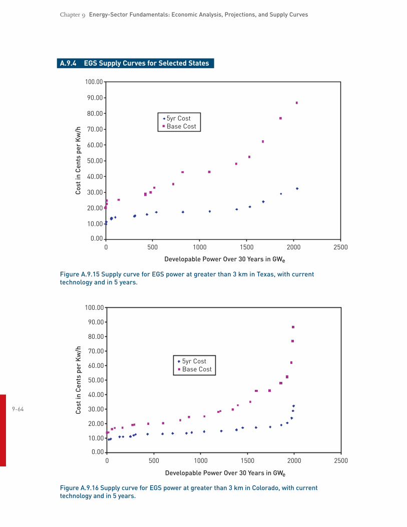
Chapter 9 EnergySector Fundamentals: Economic Analysis, Projections, and Supply Curves
A.9.4 EGS Supply Curves for Selected States
Developable Power Over 30 Years in GW
Cos
tin
Cen
tspe
rK
w/h
0 500 1000 1500 2000 25000.00
10.00
20.00
30.00
40.00
60.00
50.00
70.00
80.00
90.00
100.00
5yr CostBase Cost
e
Figure A.9.15 Supply curve for EGS power at greater than 3 km in Texas, with current technology and in 5 years.
964
Developable Power Over 30 Years in GW
Cos
tin
Cen
tspe
rK
w/h
0 500 1000 1500 2000 25000.00
10.00
20.00
30.00
40.00
60.00
50.00
70.00
80.00
90.00
100.00
5yr CostBase Cost
e
Figure A.9.16 Supply curve for EGS power at greater than 3 km in Colorado, with current technology and in 5 years.
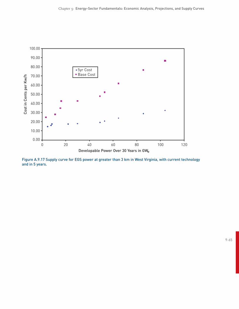
Chapter 9 EnergySector Fundamentals: Economic Analysis, Projections, and Supply Curves
5yr CostBase Cost
Developable Power Over 30 Years in GW
Cos
tin
Cen
tspe
rK
w/h
0 20 40 60 80 100 1200.00
10.00
20.00
30.00
40.00
60.00
50.00
70.00
80.00
90.00
100.00
e
Figure A.9.17 Supply curve for EGS power at greater than 3 km in West Virginia, with current technology and in 5 years.
965