Energy management strategy for fuel cell-supercapacitor ... · ... Fuel cell-supercapacitor hybrid...

Energy management strategy for fuel cell-supercapacitor hybrid

vehicles based on prediction of energy demand

Mauro G. Carignanoa,∗, Ramon Costa-Castellob, Vicente Rodac, Norberto M. Nigrod, SergioJuncoe, Diego Feroldif

aEscuela de Ingenierıa Mecanica, CONICET-FCEIA-UNR, Beruti 2109, S2000FFI, Rosario, [email protected]

bDepartament d’Enginyeria de Sistemes, Automatica i Informatica Industrial, UPC, C/Pau Gargallo 5,08028, Barcelona, Spain. [email protected]

cInstitut de Robotica i Informatica Industrial, CSIC-UPC, C/Llorens i Artigas 4-6, 08028, Barcelona, [email protected]

dCentro de Investigacion de Metodos Computacionales, CIMEC-CONICET-UNL, Colectora Ruta Nac. N 168km. 0, Pje El Pozo, Santa Fe, Argentina. [email protected]

eLAC, Laboratorio de Automatizacion y Control, FCEIA-UNR, Riobamba 245 bis, S2000EKE, Rosario,Argentina. [email protected]

fCentro Internacional Franco Argentino de Ciencias de la Informacion y de Sistemas, CIFASIS-CONICET,Ocampo y Esmeralda, S2000EZP, Rosario, Argentina. [email protected]

Abstract

Offering high efficiency and producing zero emissions Fuel Cells (FCs) represent an excellent

alternative to internal combustion engines for powering vehicles to alleviate the growing pollu-

tion in urban environments. Due to inherent limitations of FCs which lead to slow transient

response, FC-based vehicles incorporate an energy storage system to cover the fast power vari-

ations. This paper considers a FC/supercapacitor platform that configures a hard constrained

powertrain providing an adverse scenario for the energy management strategy (EMS) in terms

of fuel economy and drivability. Focusing on palliating this problem, this paper presents a

novel EMS based on the estimation of short-term future energy demand and aiming at main-

taining the state of energy of the supercapacitor between two limits, which are computed online.

Such limits are designed to prevent active constraint situations of both FC and supercapacitor,

avoiding the use of friction brakes and situations of non-power compliance in a short future

horizon. Simulation and experimentation in a case study corresponding to a hybrid electric

bus show improvements on hydrogen consumption and power compliance compared to the

widely reported Equivalent Consumption Minimization Strategy. Also, the comparison with

the optimal strategy via Dynamic Programming shows a room for improvement to the real-time

strategies.

Keywords: Fuel cell-supercapacitor hybrid vehicle, State constraint, Energy management

∗Corresponding author. Email address: [email protected], tel:+543414808536, fax:+543414802654,Beruti 2109, S2000FFI, Rosario, Argentina.

Preprint submitted to Journal of Power Sources July 5, 2017

strategy, Fuel economy, Drivability

2

1. Introduction

Fuel Cell Hybrid Vehicles (FCHV) represent a solution of increasing interest for car man-

ufacturers. Some examples are Hyundai (TUCSON), General Motors (Chevrolet Equinox),

Honda (FCX-V4 y FCX Clarity), Toyota (Toyota FCHV) and Volkswagen (Passat Lingyu).

Nevertheless, some matters associated to hydrogen (H2) production; distribution and storage;

and fuel cell cost and lifetime, must be improved to make this technology more profitable and

affordable [1]. . Fuel Cells (FCs) offer two main advantages compared to the internal com-

bustion engines: higher efficiency and zero emissions. However, despite these advantages, FCs

present some limitations associated with its slow transient response, which must be taken into

account to avoid premature aging [2, 3, 4]. Taking into account such restriction, FCHVs incor-

porate an energy storage system to cover the fast power variations. Additionally, this energy

storage system allows to recover energy from braking. In most cases, a battery is adopted for

such purpose. Despite the advances on this technology, electrochemical batteries still offer a

relative short lifetime limited to thousands of cycles [5, 6]. To solve this drawback, FCHVs

incorporate a supercapacitor (SC) to replace the battery or in combination with that [7]. In

contrast to batteries, SCs offer hundreds of thousands of duty cycles and a higher specific power

[8, 9], with the disadvantages of having lower specific energy and higher cost per unit of energy

stored.

From the point of view of the energy management strategy (EMS), FCHVs with SC represent

and adverse scenario due to the existence of active state-dependent constraints. Such constraints

affect sensitively both the H2 consumption and the fulfillment of power demand. A review

of EMS for FCHV presented in [1] indicates that the Equivalent Consumption Minimization

Strategy (ECMS) is the most outstanding strategy. There are a large number of works reported

in the literature about this strategy but most of them dealing with Engine/Battery hybrid

vehicles. In the case of FCHV with SC, the formulation differs slightly from the previous

one. Rodatz et al. [10] presents a complete description of the ECMS and the implementation,

including experimental validation, in a FCHV with SC. The performance obtained in terms

of H2 consumption shows results comparable to, but not better than, the map-based control

strategy presented in [11]. Although ECMS provides a close-to-optimal solution in a wide range

of hybrid platforms, especially in the case of using internal combustion engine and battery

[12, 13], the differences with the optimal solution increases in case of a system with active

state constraints. A comparison presented in [14] shows differences higher than 10% between

the ECMS and the optimal offline strategy. Perez et al. [15] uses Pontryagin’s minimum

3

principle to obtain offline the trajectory of the adjoint state with the purpose of improving the

performance of the ECMS in the cases of active state constraints.

In contrast to optimization approaches, rule-based strategies are also reported in the lit-

erature. This approach offers in general an acceptable performance and lower computational

burden, which become more suitable for real time application [16, 17]. Most rule-based or

mapped strategies only use the state of charge of supercapacitors and the power demand as

inputs. Feroldi et al. [18] presents a rule-based strategy based on a FC map efficiency. The

results obtained show a difference of around 6% on H2 consumption compared to the opti-

mal offline strategy. Despite the good performance obtained, the size of supercapacitor bank

adopted in [18] seems to be large enough so that no active state constraints appear, which

provides favorable conditions for the EMS.

In this work, a new EMS for a FCHV with SC based on energy estimations is presented.

The strategy is specially designed for platforms in which state-dependent constraints get often

active in operation. It uses information of the current states of the vehicle such as vehicle speed,

SC state of energy and FC power flow. The case study concerns a hybrid electric bus operated

under urban driving conditions. First, the performance of the proposed strategy is evaluated

by simulation using a quasistatic model of the powertrain, and the results are compared to

those of ECMS and to the optimal offline strategy obtained through Dynamic Programming.

Simulation results include a sensitivity analysis against changes in the driving condition and

the mass of the vehicle. Finally, an experimental validation is carried out in a hybrid power

station. The rest of the paper is organized as follows: in Section 2, the model of the FCHV

is presented; Section 3 describes the novel strategy; in Section 4, the case study is described

and the results obtained by simulations are shown; in Section 5, the experimental validation is

presented; and finally the conclusions and a prospective are drawn in Section 6.

4

2. Vehicle Model

The configuration of the FCHV adopted in this work is shown in Fig. 1. As can be observed,

the power at wheels is provided by the Electric Machine (EM) through the differential. The

EM can also work as a generator to recover energy from braking, and it is connected to the

direct current bus (DC-BUS) through a bidirectional converter. Finally, the FC delivers power

through the Boost converter to the direct current bus (DC-BUS), while the SC delivers or

receives power via the Buck/Boost converter.

The model of the powertrain used to evaluate the H2 consumption and the power compliance

focuses on the efficiency and the constraints, neglecting most of the dynamics. Some comparison

reported in the literature between quasistatic model against high order model [12] or real system

[19] show the closeness of the results. In the following all the models are formulated in discrete

time.

2.1. Supercapacitor model

An analytic expression to model the SC can be deduced from the equivalent circuit composed

of a capacitor and a resistor connected in series.

The SC current can be expressed as a function of the power demanded PSC ,

ISC(k) =USC,oc(k)− (U2

SC,oc(k)− 4PSC(k)RSC)0.5

2RSC

. (1)

where RSC is the internal resistance, USC,oc(k) = QSC(k)/CSC is the open-circuit voltage, and

QSC(k) and CSC are the charge and the capacity of the SC, respectively. As the proposed EMS

is based on energy estimations, it is appropriate to introduce the energy as a variable. Hence,

the energy stored (ESC) and the nominal energy (ESC,0) of the SC are introduced as follows:

ESC(k) = 0.5 CSC U2SC,oc(k), ESC,0 = 0.5 CSC U2

SC,0, (2)

Fuel Cell

Supercapacitor

Electric

Machine

+

Converter

Boost

converter

Differential

Buck/Boost

converter

DC-B

US

PSC

PBB

PBO

PFC

PEM

PCON

PFr-Br

Pwh

Figure 1: FCHV configuration.

5

where USC,0 is the nominal voltage. Notice that here “nominal” means fully charged. Now, the

state of energy (SOE) is the relation between the energy stored and the nominal energy of SC,

and its dynamics can be expressed as follows,

SOE(k + 1) = SOE(k)− USC,oc(k) ISC(k) tsESC,0

, (3)

where ts is the time discretization interval. With this definition, the current in the SC is

considered positive for discharging.

Concerning the constraints, fixed lower and upper limits of SOE are considered, and the

current is also limited, i.e.:

SOEmin ≤ SOE(k) ≤ SOEmax, (4)

−ImaxSC ≤ ISC(k) ≤ ImaxSC . (5)

Notice that (4) is a state constraint, and (5) is a state-dependent constraint, due to (1)-(3).

2.2. Fuel cell model

Hydrogen FCs are used to generate electricity from an electrochemical reaction between

oxygen and H2. For the purposes of this work, the FC is reduced to a quasistatic model,

including its constraints and efficiency map. Assuming that the response time of the system

is noticeably lower than the sampling time, it can be considered that the power delivered by

the FC in the each interval of time is exactly the power reference PFC(k) received as input in

the low level controller.

On the other hand, the power gradient in the FC is ∆PFC(k) = (PFC(k)− PFC(k − 1))/ts.

Then, the control input is limited to the following physical constraints:

0 ≤PFC(k) ≤ PmaxFC , (6)

∆PminFC ≤ ∆PFC(k) ≤ ∆Pmax

FC , (7)

where PmaxFC is the maximum power of the FC, and ∆Pmin

FC and ∆PmaxFC are the maximum and

minimum allowed power gradients. Currently, it is not entirely clear how to accurately establish

the power rate limits to assure non-premature ageing of FCs. Quantifying degradation in FCs

is a complex task because the degradation rate strongly depends on the internal conditions

[20, 21]. Although some authors do not consider power rate constraints in the fuel cell [22,

23, 24, 25], values between 2% and 20% of its maximum power per second are usually adopted

[26, 27, 10, 18, 28, 29, 14, 30]. In this work, a maximum of 10% of the maximum power of

the FC per second for rising and falling is assumed . Notice that the constraint given by (7)

6

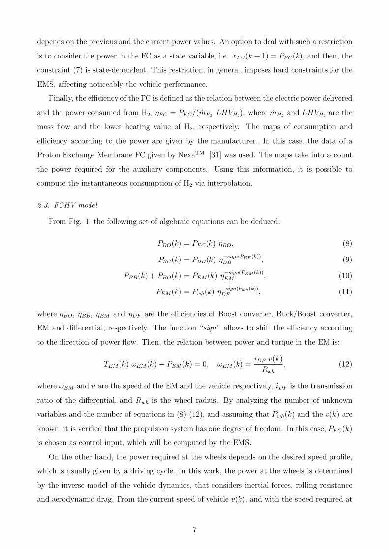
depends on the previous and the current power values. An option to deal with such a restriction

is to consider the power in the FC as a state variable, i.e. xFC(k + 1) = PFC(k), and then, the

constraint (7) is state-dependent. This restriction, in general, imposes hard constraints for the

EMS, affecting noticeably the vehicle performance.

Finally, the efficiency of the FC is defined as the relation between the electric power delivered

and the power consumed from H2, ηFC = PFC/(mH2 LHVH2), where mH2 and LHVH2 are the

mass flow and the lower heating value of H2, respectively. The maps of consumption and

efficiency according to the power are given by the manufacturer. In this case, the data of a

Proton Exchange Membrane FC given by NexaTM [31] was used. The maps take into account

the power required for the auxiliary components. Using this information, it is possible to

compute the instantaneous consumption of H2 via interpolation.

2.3. FCHV model

From Fig. 1, the following set of algebraic equations can be deduced:

PBO(k) = PFC(k) ηBO, (8)

PSC(k) = PBB(k) η−sign(PBB(k))BB , (9)

PBB(k) + PBO(k) = PEM(k) η−sign(PEM (k))EM , (10)

PEM(k) = Pwh(k) η−sign(Pwh(k))DF , (11)

where ηBO, ηBB, ηEM and ηDF are the efficiencies of Boost converter, Buck/Boost converter,

EM and differential, respectively. The function “sign” allows to shift the efficiency according

to the direction of power flow. Then, the relation between power and torque in the EM is:

TEM(k) ωEM(k)− PEM(k) = 0, ωEM(k) =iDF v(k)

Rwh

, (12)

where ωEM and v are the speed of the EM and the vehicle respectively, iDF is the transmission

ratio of the differential, and Rwh is the wheel radius. By analyzing the number of unknown

variables and the number of equations in (8)-(12), and assuming that Pwh(k) and the v(k) are

known, it is verified that the propulsion system has one degree of freedom. In this case, PFC(k)

is chosen as control input, which will be computed by the EMS.

On the other hand, the power required at the wheels depends on the desired speed profile,

which is usually given by a driving cycle. In this work, the power at the wheels is determined

by the inverse model of the vehicle dynamics, that considers inertial forces, rolling resistance

and aerodynamic drag. From the current speed of vehicle v(k), and with the speed required at

7

next step vreq(k + 1), the power required at the wheels (P reqwh ) is computed using the following

set of equations:

a(k) = (vreq(k + 1)− v(k)) t−1s ,

Finer(k) = m a(k),

Faero(k) = 0.5 Af Cx ρair v(k)2,

Froll(k) = m g (r0 + r1 v(k)),

Fwh(k) = Faero(k) + Froll(k) + Finer(k),

P reqwh (k) = Fwh(k) v(k),

(13)

where a is the linear acceleration; m is the total mass of the vehicle; Af , Cx and ρ are frontal

area, drag coefficient and air density respectively; r0 and r1 are rolling resistance coefficients;

and g is the acceleration of gravity.

It is necessary to know the power demanded at the wheels to compute the EMS. Before

using P reqwh , it is bounded according to the power available from the propulsion system. The

maximum (and minimum) power available at each time depends on the physical limitations of

the components. Table 1 summarizes the constraints of the propulsion system. Taking into

account these constraints, it is possible to compute at each time the maximum and minimum

power available at wheel, namely Pmaxwh and Pmin

wh . It is worth to notice that these values depend

on the vehicle speed, and on the state variables xFC and SOE. The power available at the

Table 1: Constraints in the propulsion system.

Variable min. max.

EM Torque, TEM −TmaxEM TmaxEM

EM Power, PEM −PmaxEM Pmax

EM

FC power, PFC 0 PmaxFC

FC gradient, ∆PFC ∆PminFC ∆Pmax

FC

Buck/Boost Power, PBB −PmaxBB Pmax

BB

SC current, ISC −ImaxSC ImaxSC

SC energy, SOE SOEmin SOEmax

wheels is directly related to the drivability (speed compliance) and to the global efficiency. It

means that, in case of propulsion, when P reqwh is higher than Pmax

wh , the future speed achieved

will be lower than the speed required. On the contrary, in case of regenerative braking, when

Pminwh is higher than the power required, the friction brakes must be employed. Finally, the

8

power required at the wheels given by (13) is bounded as follows:

Pwh(k) = maxminP reqwh (k);Pmax

wh (k);Pminwh (k), (14)

and the power dissipated on the friction brakes results:

PFr−Br(k) =

0, if P reqwh (k) ≥ 0,

Pminwh (k)− P req

wh (k), if P reqwh (k) < 0.

(15)

Figure 2 shows a schematic representation of the causal model used to perform the simulations.

Notice that, if the power required is lower than the power available, a new value of future speed

is computed by using the longitudinal vehicle model. The block named “Power balance” in

Fig. 2 refers to the set of equations (8)-(11).

Pwh

req

(k)SC

PSC (k)

PFC (k)

SOE(k+1)

xFC (k)

vreq (k+1)

v(k+1)

PFr-Br (k)

v(k)

speed

mH2(k)

Inverse

longitudinal

vehicle model

xFC (k+1)Energy

Management

Strategy

Power available

according to

the constraints

SOE(k)

Pwh(k)

FC

Longitudinal

vehicle model

v(k)

Power

balance

Figure 2: Schematic representation of the model to perform the simulations.

9

3. Energy-based Estimation Strategy

The EMS proposed in this work, named hereafter Energy-Based Estimation Strategy (EBES),

has three goals: i) to provide at any time the power required to propel the vehicle; ii) to recover

as much energy as possible from braking; and iii) to operate the fuel cell at maximum efficiency.

Figure 3 shows the flowchart of the strategy. In the first step, two SOE limits are computed

using the current speed and the state of the FC. Then, by comparing such values with the

current SOE, and taking into account the power demanded at wheel, the FC power reference

(uFC) is computed. Finally, the power value for the FC is bounded according to the constraints

of the propulsion system. The procedure to compute the SOE limits is described below.

Compute FC power

reference

Apply bounds according

to the constraints

SOE(k) v(k) xFC(k)

PFC (k)

Compute SOE limits

SOElow(k) SOEhi(k)

uFC (k)

Pwh(k)

Figure 3: Flowchart of the Energy-based Estimation Strategy.

3.1. Determination of the supercapacitor SOE limits

This stage is the core of the strategy, in which, an upper and a lower limit of SOE, namely

SOEhi and SOElow, are found. In contrast to previous published strategies (for example in

[18]), in this work such limits are not fixed, but they are adapted during runtime according to

the vehicle speed and FC power state. Specifically, these limits are computed so that if the

current SOE is between SOEhi and SOElow, the propulsion system is able to accelerate from

the current speed up to a predefined maximum speed; and also it is able to store overall energy

produced by both the regenerative braking and FC from the current speed until the vehicle

stops. Accordingly, the first step to know such limits is to estimate the energy required for the

vehicle in a short future period of time to change its speed.

3.1.1. Trip energy estimation

Hereafter the term “trip” will be used to refer to hypothetical short time displacement in

which the vehicle accelerates o decelerates uniformly from a given current speed until a certain

10

xFC (k)

PFC

max

tg()=PFC

max

tmax FC

tpr

FC Power

Time

350 360 370 380 390 400 410 420 430 440 450

time [s]

0

2

4

6

8

10

12

14

16Speed [

ms-1

]

current

speed

hypothetical

braking

trip

hypothetical

propulsion

trip

real future

speed

(a)

(b)

Figure 4: (a) Hypothetical future trips from the current speed, (b) Evolution of FC power from current state

to maximum power.

future speed (see Fig. 4-(a)).

An estimation of the energy required during a trip from an initial speed v0 to a final speed vf

can be done considering the variation of kinetic energy. However, such approximation neglects

the dissipation effects produced by aerodynamics and rolling resistances. A more accurate

estimation is obtained taking into account such effects. Then, the total energy required (at the

wheels) is the sum of the three terms:

Etrip = Ekin + Eaero + Eroll, (16)

where Ekin, Eaero and Eroll are the kinetic energy variation, the energy dissipated by aerody-

namics effect, and the energy dissipated by rolling resistance respectively. Notice that Eaero

and Eroll are always positive, while Ekin depends on whether it is a propulsion trip (positive) or

a braking trip (negative), and therefore Etrip might be positive or negative. The kinetic energy

variation from v0 to vf is

Ekin = 0.5 m(v2f − v20

). (17)

Then, the energy dissipated by aerodynamics effect during a trip is

Eaero(t) =

∫ t

0

Caero v3(τ) dτ, (18)

where Caero = 0.5 Af Cx ρair. From v0, and assuming a constant acceleration a during the trip,

(18) results:

Eaero(t) =

∫ t

0

Caero (v0 + a τ)3 dτ, (19)

and solving the definite integral leads to:

Eaero(t) = Caero

(a3 t4

4+ a2 t3 v0 +

3 a t2 v202

+ t v30

). (20)

11

Then, assuming a final speed vf , the time required to reach such speed is t = (vf − v0)/a. Re-

placing in (20) and by algebraic simplification, the expression to compute the energy dissipated

by aerodynamics results:

Eaero =Caero4 a

(v4f − v40

). (21)

For the rolling resistance, a similar procedure is used. From an initial speed and constant

acceleration, the energy dissipated results:

Eroll(t) =

∫ t

0

m g (r0 + r1 v(τ)) v(τ) dτ

= m g

∫ t

0

r0 (v0 + a τ) + r1 (v0 + a τ)2 dτ

(22)

and solving the definite integral leads to:

Eroll(t) = mg(

(r0v0 + r1v20) t+

(r0 + 2v0r1) a.t2

2+r1a

2t3

3

), (23)

and, with t = (vf −v0)/a, the expression to compute the energy dissipated by rolling resistance

results:

Eroll =mg

a

(r1(v

3f − v30)

3+r0(v

2f − v20)

2

). (24)

According to (21) and (24), it is easy to verify that the effect of the aerodynamic and rolling

resistances in the trip energy increases as the acceleration (in absolute value) decreases.

Summarizing, from (17), (21) and (24) it is possible to compute, analytically, an estimation

of the energy required in a trip, by using the initial and final speed, the acceleration and the

vehicle parameters.

3.1.2. Lower state of energy

The lower state of energy, namely SOElow, is computed so that if the current SOE is

higher than SOElow, the propulsion system is able to provide the energy required to go from

the current speed up to a maximum predefined speed (vmax). During a propulsion trip, the

energy required at the wheels is computed from (16), with v0 = v(k), vf = vmax and a = apr,

where apr and vmax are adjustable parameters. Then, using the efficiencies of the components,

the energy required from DC-BUS results:

Epr(k) =Etrip(k)

ηDF ηEM. (25)

This energy drawn from the DC-BUS must be supplied by the FC and the SC, which leads to:

ESC(k) ηSC ηBB + EprFC(k) ηBO ≥ Epr(k), (26)

12

where ESC is the energy available in the SC, ηSC is the average efficiency of SC, and EprFC is

the maximum energy that the FC is able to provide during this trip. The latter is computed

assuming that the FC rises up to its maximum power from its current state as fast as possible.

Therefore, EprFC can be computed as the area under the curve showed in the Fig. 4-(b), which

leads to:

EprFC(k) =

tmaxFC (k)

(PmaxFC +xFC(k)

2

)+ (tpr(k)− tmaxFC (k)) Pmax

FC if tpr(k) ≥ tmaxFC (k),

tpr(k)(PmaxFC (k)+xFC(k)

2

)if tpr(k) < tmaxFC (k).

(27)

Here, tmaxFC is the time the FC takes to reach the maximum power, and tpr is the time the trip

takes from v(k) up to vmax with constant acceleration apr:

tmaxFC (k) =PmaxFC − xFC(k)

∆PmaxFC

; tpr(k) =vmax − v(k)

apr. (28)

Although in Fig. 4 tpr is higher than tmaxFC , the opposite situation is also possible, which

corresponds to the second case of (27). Now, from (26) and with the definition of SOE, it

follows that:

SOE(k) ≥

(Epr(k)− Epr

FC(k) ηBOηSC ηBB ESC,0

). (29)

Notice that by fulfilling this expression, the propulsion system has enough energy to propel the

vehicle from the current speed until vmax with the constant acceleration apr. Then, taking into

account the minimum SOE allowed in the SC, the lower SOE due to energy is defined as:

SOElow,E(k) =

(Epr(k)− Epr

FC(k) ηBOηSC ηBB ESC,0

)+ SOEmin. (30)

So far, the condition SOE(k) ≥ SOElow,E(k) assures that the vehicle has the required energy

for the trip, i.e. the constraint associated with SOE will not be activated. In addition, the

constraint associated with the maximum SC current is potentially activated, specially when

SOE is low, because the voltage falls and the current rises noticeably. To avoid that, a lower

SOE by current, namely SOElow,I , must be found. It is defined in such a way that when

SOE(k) > SOElow,I , a power flow in the Buck/Boost equal to PmaxBB produces a current on the

SC side lower than ImaxSC . From the SC model, it leads to:

SOE(k) ≥

(PmaxBB

ηBB ImaxSC

+RSC ImaxSC

)2CSC

2ESC,0, (31)

where the right-hand term is the lower limit by current:

SOElow,I =

(η−1BBP

maxBB

ImaxSC

+RSC ImaxSC

)2CSC

2ESC,0. (32)

13

Notice that, unlike (30), this expression does not depend on k. Finally, the lower SOE limit

for the strategy is computed as follows:

SOElow(k) = maxSOElow,E(k);SOElow,I. (33)

3.1.3. Higher state of energy

The higher state of energy, namely SOEhi, is computed so that if the current SOE is lower

than SOEhi, the SC is able to recover all the energy from the wheels and from the FC during

a braking trip from the current speed until the vehicle stops. This condition can be expressed

as follows:ESC,0 − ESC(k)

ηSC≥(Ebr(k) + Ebr

FC(k) ηBO)ηBB, (34)

where the left hand side represents the maximum energy that can be stored in the SC from the

current SOE; Ebr is the energy delivered to the DC-BUS from the regenerative braking; and

EbrFC is the minimum energy delivered by the FC during this trip. Now, solving for ESC from

(34), and expressing ESC in term of SOE, (34) leads to:

SOE(k) ≤ 1−(Ebr(k) + Ebr

FC(k) ηBO)ηBB ηSC

ESC,0. (35)

In this expression, Ebr(k) is computed from (16), with v0 = v(k), vf = 0 and a = abr, where

abr is an adjustable parameter. Then, using the efficiencies of the components, Ebr(k) results:

Ebr(k) = −Etrip(k) ηDF ηEM . (36)

Then, to compute EbrFC , it is assumed that from the current power state, the FC falls down to

zero as fast as possible, resulting in:

EbrFC(k) =

x2FC(k)

−2 ∆PminFC

. (37)

Notice that by fulfilling (35), the SC is able to store all the energy from the wheels and the

FC during a braking trip from the current speed until it stops. Therefore, the higher SOE

reference of the strategy is:

SOEhi(k) = 1−(Ebr(k) + Ebr

FC(k) ηBO)ηBB ηSC

ESC,0. (38)

So far, the expressions to compute SOElow and SOEhi were deduced. These expressions, in

addition to the vehicle parameters, include the current speed and the current power flow in the

FC. Accordingly, SOElow and SOEhi are adapted during runtime. These limits have a different

meaning to SOEmin and SOCmax: the last ones provide the operation limits of the SC (see

Eq. 4), while SOElow and SOEhi provide information to the proposed strategy to compute the

power required from the FC.

14

3.2. Fuel cell power reference

Once the SOE limits were computed, the current state of the propulsion system is classified

into one of the three modes:Overcharged, if SOE(k) > SOEhi(k),

Charged, if SOElow(k) ≤ SOE(k) ≤ SOEhi(k),

Discharged, if SOE(k) < SOElow(k).

Then, according to the current mode, the FC power reference is computed as follows:

uFC(k) =

0, if Overcharged,

min

maxP lowchg ; Pwh(k)

ηFC,wh

;P hi

chg

, if Charged,

maxPwh(k)ηFC,wh

;Pdis

, if Discharged,

(39)

where P lowchg , P hi

chg and Pdis are adjustable parameters, and ηFC,wh is the efficiency of the electrical

path from the FC to the wheels (ηFC,wh = ηBO ηEM ηDF ). In Overcharged mode, setting FC

power reference equal to zero aims to avoid the SOE increment. Then, in Charged mode, the

objective is to remain in this mode, and therefore, a tracking of the power demanded is intended

by setting the FC power reference equal to Pwh(k)/ηFC,wh. In addition, in this mode, the power

reference is bounded by P lowchg and P hi

chg to avoid operating the FC at low efficiency. Finally, in

Discharged mode, a tracking of the power demanded is intended, including a lower bounded,

which aims to increase the SOE.

So far, the FC power reference was determined in order to: first, maintain the SOE between

SOEhi and SOElow; and second, operate the FC at high efficiency. Before using this value

as a power reference to the FC, it must be bounded to satisfy the multiple constraints of the

propulsion system. The maximum and minimum FC power that satisfy the constraints, namely

umaxFC (k) and uminFC (k), can be obtained by means of (8)-(12). Notice that these values depend

on: the previous state of power in the FC, the state of energy of the SC and the power demand

at the wheels. Finally, the power assigned to the FC results:

PFC(k) = maxminuFC(k);umaxFC (k);uminFC (k). (40)

15

4. Simulation results

The performance of the proposed strategy is evaluated under real driving conditions in

two stages: first, by simulation, then, through experimental tests (Section 5). The results are

compared with those obtained with the ECMS and with the optimal strategy obtained by using

Dynamic Programming. The case study is described below.

4.1. Case study

The FCHV corresponds to a city bus. The sizing of FC and SC was addressed following the

guidelines reported by [14]. Basically, the FC has power enough to maintain a constant speed

of 60 kmh−1 (without using the SC). With this sizing, the maximum power of the FC results

significantly higher than the average power consumed by the bus during the cycles, while the

size of the SC is a trade-off decision between fuel economy and SC costs. The parameters of

FCHV are listed in Table 2.

In this work, two urban driving cycles are used to evaluate the performance of the strategies.

The first one is the standard speed profile Manhattan Bus Cycle (MBC) [33], while the second

one corresponds to a cycle of buses in the city of Buenos Aires, namely Buenos Aires Bus Cycle

(BABC) 1 [12]. Table 3 summarizes the main properties of the driving cycles, while the speed

profiles are shown below.

4.2. Adjustment of the strategies and performance indicators

Both strategies, EBES and ECMS, require the adjustment of some parameters. In order

to realize a fair comparison, they must be properly tuned. In this work, a parametric sweep

is used to determine the optimal tuning. The procedure consists in evaluating repeatedly

the performance of the strategy under the same driving conditions varying the adjustable

parameters in order to cover all the feasible possibilities. In this case, the driving cycle chosen

is MBC. Moreover, to reduce the simulation time, only the parameters with high sensitivity are

included in the parametric sweep. In the case of EBES the parameters varied are vmax, Plowchg ,

P hichg and Pdis, while apr and abr remain constant equal to 0.8 and -1.1ms−2, respectively. On the

other hand, for the strategy ECMS, the parameters with higher sensitivity are the equivalence

factor for discharge (sdis); the equivalence factor for charge (schg); the time horizon (th); and

the reference of state of energy in the SC, (SOEref ). More details about these parameters

are found in [10]. For this strategy, many procedures to adjust the equivalence factors are

1It was created and provided by ITBA, Instituto Tecnologico de Buenos Aires.

16

Table 2: FCHV parameters: chassis, EM, differential and electronic converters are from AutonomyTM [32]; FC

efficiencies from [31]; and SC from [9].

Description Parameter Value Unit

Cargo mass mcargo 2400 kg

Chassis mass mch 11250 kg

Frontal area Af 8.06 m2

Drag coefficient Cx 0.65 -

Rolling coefficientr0 0.008 -

r1 0.00012 sm−1

Wheel radius Rwh 0.51 m

Differential, ratio iDF 12.3 -

Differential, Effic. ηDF 0.95 -

EM, Power max. PmaxEM 100 kW

EM, Torque max. TmaxEM 1380 N m

EM, Effic. ηEM 0.88 -

FC, Power max. PmaxFC 48 kW

FC, Power rise. max. ∆PmaxFC 4.8 kW s−1

FC, Power fall. max. ∆PminFC -4.8 kW s−1

FC, Max. efficiency - 52 %

FC, Eff. at max power - 40 %

Boost, Power max. PmaxBO 50 kW

Boost, Effic. ηBO 0.95 -

SC, cells in series N cellser 130 -

SC, branches in parallel N branchpar 2 -

SC, cell rated capacity CcellSC 2700 F

SC, cell resistance RcellSC 0.001 Ω

SC, cell nominal voltage U cellSC 2.5 V

SC, current max. ImaxSC 350 A

SC, SOE min. SOEmin 0.25 -

SC, SOE max. SOEmax 1 -

Buck/Boost, Power max. PmaxBB 75 kW

Buck/Boost, Effic. ηBB 0.95 -

17

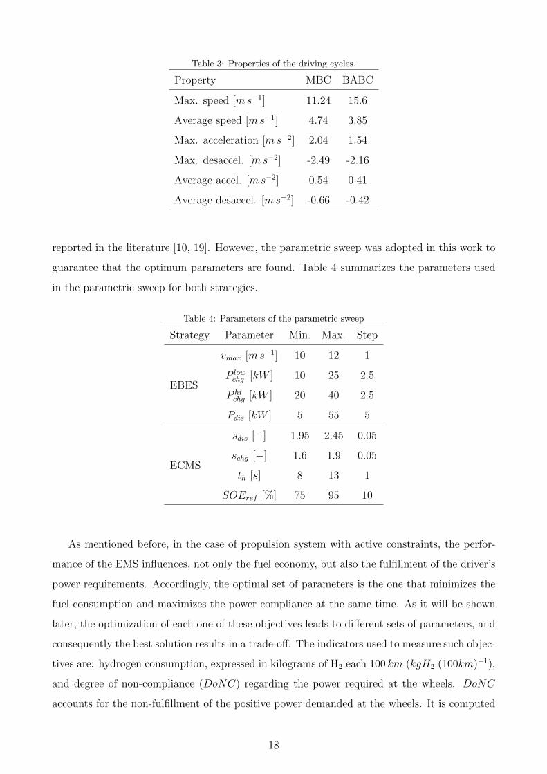
Table 3: Properties of the driving cycles.

Property MBC BABC

Max. speed [ms−1] 11.24 15.6

Average speed [ms−1] 4.74 3.85

Max. acceleration [ms−2] 2.04 1.54

Max. desaccel. [ms−2] -2.49 -2.16

Average accel. [ms−2] 0.54 0.41

Average desaccel. [ms−2] -0.66 -0.42

reported in the literature [10, 19]. However, the parametric sweep was adopted in this work to

guarantee that the optimum parameters are found. Table 4 summarizes the parameters used

in the parametric sweep for both strategies.

Table 4: Parameters of the parametric sweep

Strategy Parameter Min. Max. Step

EBES

vmax [ms−1] 10 12 1

P lowchg [kW ] 10 25 2.5

P hichg [kW ] 20 40 2.5

Pdis [kW ] 5 55 5

ECMS

sdis [−] 1.95 2.45 0.05

schg [−] 1.6 1.9 0.05

th [s] 8 13 1

SOEref [%] 75 95 10

As mentioned before, in the case of propulsion system with active constraints, the perfor-

mance of the EMS influences, not only the fuel economy, but also the fulfillment of the driver’s

power requirements. Accordingly, the optimal set of parameters is the one that minimizes the

fuel consumption and maximizes the power compliance at the same time. As it will be shown

later, the optimization of each one of these objectives leads to different sets of parameters, and

consequently the best solution results in a trade-off. The indicators used to measure such objec-

tives are: hydrogen consumption, expressed in kilograms of H2 each 100 km (kgH2 (100km)−1),

and degree of non-compliance (DoNC) regarding the power required at the wheels. DoNC

accounts for the non-fulfillment of the positive power demanded at the wheels. It is computed

18

as follows:

DoNC[%] =

(1−

∑Nk=1 P

+wh(k)∑N

k=1 Preq+wh (k)

)× 100, (41)

where the superscript ‘+’ means that only positive powers are included in the sum. With this

definition, a DoNC = 0% means that the power required was fulfilled throughout the cycle, i.e.

full compliance of the speed required. Another useful measurement to analyze the performance

of the strategies is the amount of energy recovered from braking. In this case a new indicator,

named degree of recovered energy (DoRE), is defined:

DoRE[%] =

∑Nk=1 P

−wh(k)∑N

k=1 Preq−wh (k)

× 100, (42)

where the superscript ‘-’ means that only negative powers are included in the sum. With this

definition, a DoRE = 100% means that the friction brakes are not used, and all the energy

from braking was recovered in the SC. These indicators (DoRE and DoNC) were introduced

in a previous work [14], with a slight variation in their definition, but with the same meaning.

Regarding the fuel consumption, to make a fair comparison, the difference between the

initial SOE and the SOE at the end of the cycle is compensated by adding (or subtracting)

an amount of H2 to the H2 consumed. Such compensation was made by using two equivalence

factors computed from the efficiency of the components of the propulsion system, as explained

in [19]. Accordingly, when the final SOE is lower than the initial SOE, the equivalence factor

is equal to 1.96, while if the final SOE is higher than the initial one, the equivalence factor

used is 1.59.

Concerning the optimal strategy, Dynamic Programming was implemented using xFC and

SOE as state variables, PFC as control input, and the H2 consumption as cost function. A

vectorized implementation has been adopted according to guidelines from [34]. In the next

section, the performance obtained with the different strategies are compared.

4.3. Results

For a better understanding of the proposed strategy, Fig. 5-(a) shows a segment of simula-

tions using EBES where the three modes of the strategy appear. In this figure it can also be

observed that the required speed was not achieved around t = 430 s and t = 490 s .

Now, the results obtained from the parametric study are presented according to the per-

formance in terms of fuel consumption and DoNC. Note that we deal with a two objective

problem, in which both the fuel consumption and the DoNC are minimized. The results are

shown in Fig. 5-(b). In this figure, the Pareto front is also included, which is the set of the

19

Table 5: Performance of the strategies over MBC.

StrategyConsumption

[kgH2 (100km)−1]

Difference in

consumption

[%]

DoNC

[%]

DoRE

[%]

EBES 6.34 0 3.65 83.4

ECMS 6.47 +2.1 4.55 82.5

Optimal strategy 6.19 -2.4 1.73 84.5

Pareto-optimal points for each strategy [35]. In this work, a point is considered Pareto-optimal

if no other point exists with lower DoNC and lower Consumption at a time.

First, it can be observed that the proposed strategy presents a lower dispersion both in fuel

consumption and in DoNC, compared to the ECMS. It means that in the case of a non-optimal

adjustment of its parameters, EBES presents a lower loss of performance, which is desirable.

Then, the lower consumption is obtained with the EBES, which is around 6.34 kgH2 (100km)−1,

while the DoNC is 3.6%. The minimum DoNC is similar in both strategies, around 3.3%.

However, in the case of ECMS, the consumption increases notably at lower values of DoNC.

Now, a single set of parameters is chosen for each strategy. It is reasonable to choose a

set of parameters corresponding to a point in the middle of the Pareto front for each strategy,

which provides a trade-off solution between fuel economy and power compliance. Hence, the

parameters of the EBES finally adopted are vmax = 12ms−1, P lowchg = 15 kW , P hi

chg = 30 kW , and

Pdis = 15 kW ; while for the ECMC the parameters are sdis = 2.05, schg = 1.7, th = 11 s, and

SOEref = 0.85. Table 5 summarizes the results obtained using these parameters on MBC. The

second column shows the differences on fuel consumption with respect to EBES. In this Table,

the results of the optimal strategy obtained offline via Dynamic Programming are also included.

As expected the performance obtained with the optimal solution shows a lower value of DoNC

and an improvement of fuel economy with respect to EBES. These results are consistent with

the DoRE, in which the optimal strategy presents the maximum percentage of energy recovered

from braking.

Then, to analyze the sensitivity of the strategies against different driving cycle conditions,

they are tested using the cycle BABC, keeping the parameters adjusted for MBC. Table 6 shows

the result obtained. In this case, the difference on fuel consumption between the two real-time

strategies is slightly lower for the ECMS. However it presents a high DoNC. In this respect,

the proposed strategy is notably better than the ECMS. High values of DoNC mean a poor

20

0

5

10

15

Speed [m

s-1]

Reference

Attainable

0.4

0.6

0.8

1

SO

E [-]

380 400 420 440 460 480 500 520

Time [s]

0

10

20

30

40

50

FC

pow

er

[kW

]

SOE

SOElow

SOEhi

Overcharged

Charged

Discharged

6.3 6.35 6.4 6.45 6.5 6.55 6.6 6.65

Consumtion [kgH2 (100km)-1]

3

3.5

4

4.5

5

5.5

6

6.5

7

Do

NC

[%

]

EBES cloud of points

EBES Pareto front

ECMS cloud of points

ECMS Pareto front

(a)

(b)

Figure 5: (a) Segment of simulation over BABC using EBES with parameters vmax = 12ms−1, P chglow = 24 kW ,

P chghi = 26 kW and Pdis = 30 kW . (b) Performances of the strategies from a parametric sweep over MBC.

21

Table 6: Performance of the strategies over BABC.

StrategyConsumption

[kgH2 (100km)−1]

Difference in

consumption

[%]

DoNC

[%]

DoRE

[%]

EBES 6.18 0 7.75 85.4

ECMS 6.14 -0.6 14.3 86.6


drivability, which is reflected in the loss of reference speed, as shown in the Fig. 6. Note that

a lower power compliance leads to a lower consumption. Such assertion can be illustrated by a

simple example. It consists on runing the simulation with the EBES, but instead of using the

original BABC, the speed profile achieved by the ECMS is adopted. In this case, the EBES

fully complies with the cycle, and the fuel consumption is 5.96 kgH2 (100km)−1, i.e. 3.2% lower

than ECMS. Additionally, a saving of 4.8% is achieved with the optimal solution compared

to the EBES, with similar performance in terms of power compliance. The correspondence

between the H2 consumption and the energy recovered is consistent.

Finally, the sensitivity of the strategies against the total mass of the vehicle is analyzed. As

mentioned previously, the FCHV corresponds to a real bus used for urban transport, whereby

a high variation of the cargo mass (mcargo) is expected due to the variation of passengers

transported. A variation of 100% of mcargo is proposed. In the previous simulations mcargo =

2400 kg was used, which corresponds to the average of passengers, and with this value the total

vehicle mass results m = mch + mcargo = 13650 kg. Now, mmincargo = 0 kg and mmax

cargo = 5800 kg

are evaluated, which correspond to empty and full of passengers, respectively. This variation in

the cargo mass affects the total mass in a quantity ∆ = ±18% around the nominal vehicle mass

(13650 kg). Note that the variation of this parameter was made only in the vehicle dynamic

model, which affects the power required, while the strategies are computed using the same

nominal value of total mass than in the previous simulations (since it would not be practical to

measure the mass while the bus is running). The results obtained are summarized in Tables 7

and 8. As observed, the proposed strategy keeps the advantage of fuel economy and power

compliance over ECMS, even under hight variation of cargo mass. Alternatively, the optimal

strategy performs the lower fuel consumption keeping the lower level of DoNC. In Table 8,

a second optimal result is included to emphasize the effect of the power compliance on the

fuel consumption. This result is obtained by using the speed achieved by EBES as reference,

22

Time [s]

0 200 400 600 800 1000 1200 1400 1600 1800

Sp

ee

d [

ms

-1]

0

2

4

6

8

10

12

14

16

EBES

ECMS

Reference

350 400 450

Sp

ee

d [

ms

-1]

0

2

4

6

8

10

12

14

16

Time [s]

680 720 7600

2

4

6

8

10

12

14

16

1440 1460 1480 15000

2

4

6

8

10

12

14

16

Figure 6: Loss of the speed reference in BABC.

Table 7: Performance over MBC with mcargo = 0 kg.

StrategyConsumption

[kgH2 (100km)−1]

Difference in

consumption

[%]

DoNC

[%]

DoRE

[%]

EBES 5.01 0 2.82 91.3

ECMS 5.14 +2.6 6.15 88.9


23

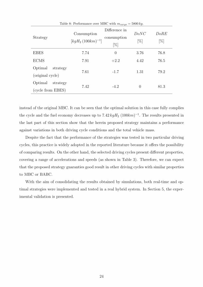
Table 8: Performance over MBC with mcargo = 5800 kg.

StrategyConsumption

[kgH2 (100km)−1]

Difference in

consumption

[%]

DoNC

[%]

DoRE

[%]

EBES 7.74 0 3.76 76.8

ECMS 7.91 +2.2 4.42 76.5

Optimal strategy

(original cycle)7.61 -1.7 1.31 79.2

Optimal strategy

(cycle from EBES)7.42 -4.2 0 81.3

instead of the original MBC. It can be seen that the optimal solution in this case fully complies

the cycle and the fuel economy decreases up to 7.42 kgH2 (100km)−1. The results presented in

the last part of this section show that the herein proposed strategy maintains a performance

against variations in both driving cycle conditions and the total vehicle mass.

Despite the fact that the performance of the strategies was tested in two particular driving

cycles, this practice is widely adopted in the reported literature because it offers the possibility

of comparing results. On the other hand, the selected driving cycles present different properties,

covering a range of accelerations and speeds (as shown in Table 3). Therefore, we can expect

that the proposed strategy guaranties good result in other driving cycles with similar properties

to MBC or BABC.

With the aim of consolidating the results obtained by simulations, both real-time and op-

timal strategies were implemented and tested in a real hybrid system. In Section 5, the exper-

imental validation is presented.

24

5. Experimental validation

The experimental validation was carried out in the Fuel Cell Laboratory belonging to the

Institut de Robotica i Informatica Industrial (IRI) from the Technical University of Catalonia

(UPC), in Barcelona, Spain. The objectives are to verify the feasibility of the proposed EMS

and the simulation results. The station used is a hybrid testing bench that uses a FC as

primary energy source and a SC as energy storage system, while the load is generated by a

programmable Source/Sink.

5.1. Description of the station

The test station used is shown in Fig. 7-(a). It is composed by the following compo-

nents: a fuel cell NexaTM model 310-0027, type proton exchange membrane, of 26 VDC, 46 A

and 1200 W; a supercapacitor module MaxwellTM model BMOD0165, type electrical double

layer, of 165 F and 48 V; a three-phase DC-DC converter SemikronTM, model SKS 75F B6CI

40 V12, of 75 A and 513 VDC; a programmable Source/Sink Hcherl & Hackl GMBHTM, model

NL1V80C40, of 80 VDC, 40 A and 3200 W; and controller National InstrumentsTM model Com-

paq Rio 9035 which has CPU Dual-Core of 1.33 GHz and a FPGA Xilinx Kintex-7 7K70T.

Fuel Cell

Supercapacitor

Electric

Machine

+

Converter

Boost

converter

Dierential

Buck/Boost

converter

DC

-BU

S

Source/Sink

3200W

Host computer

+

LABVIEW™

Fuel cell 1200W

Supercapacitor

165F, 48.5V

Three-phase

DC-DC converter DC-BUS

75V

Scaled reality Emulated

ControllerPFC

PSource/sink

Measurements

Fuel cell

NEXA™

Supercapacitor

Maxwell™

Conveter DC-DC

Semikron™

Source/Sink

H&H GMBH™

Controller

Compaq Rio 9035

National Instruments™

(a) (b)

Figure 7: (a) Fuel Cell/Supercapacitor hybrid testing bench, (b) Experimental setup

Figure 7-(b) shows the adopted experimental setup. As can be seen, most of the components

of the FCHV are present in the test station, with the exception of the EM and differential.

Therefore, the power delivered/consumed by the EM to/from the DC-BUS is emulated using

the Source/Sink. The reference power to the Source/Sink is computed from a host computer,

where the driver, differential, EM and converter are simulated in LABVIEWTM. The EMS is

25

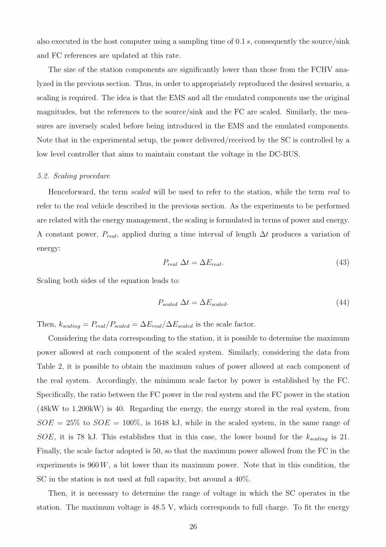
also executed in the host computer using a sampling time of 0.1 s, consequently the source/sink

and FC references are updated at this rate.

The size of the station components are significantly lower than those from the FCHV ana-

lyzed in the previous section. Thus, in order to appropriately reproduced the desired scenario, a

scaling is required. The idea is that the EMS and all the emulated components use the original

magnitudes, but the references to the source/sink and the FC are scaled. Similarly, the mea-

sures are inversely scaled before being introduced in the EMS and the emulated components.

Note that in the experimental setup, the power delivered/received by the SC is controlled by a

low level controller that aims to maintain constant the voltage in the DC-BUS.

5.2. Scaling procedure

Henceforward, the term scaled will be used to refer to the station, while the term real to

refer to the real vehicle described in the previous section. As the experiments to be performed

are related with the energy management, the scaling is formulated in terms of power and energy.

A constant power, Preal, applied during a time interval of length ∆t produces a variation of

energy:

Preal ∆t = ∆Ereal. (43)

Scaling both sides of the equation leads to:

Pscaled ∆t = ∆Escaled. (44)

Then, kscaling = Preal/Pscaled = ∆Ereal/∆Escaled is the scale factor.

Considering the data corresponding to the station, it is possible to determine the maximum

power allowed at each component of the scaled system. Similarly, considering the data from

Table 2, it is possible to obtain the maximum values of power allowed at each component of

the real system. Accordingly, the minimum scale factor by power is established by the FC.

Specifically, the ratio between the FC power in the real system and the FC power in the station

(48kW to 1.200kW) is 40. Regarding the energy, the energy stored in the real system, from

SOE = 25% to SOE = 100%, is 1648 kJ, while in the scaled system, in the same range of

SOE, it is 78 kJ. This establishes that in this case, the lower bound for the kscaling is 21.

Finally, the scale factor adopted is 50, so that the maximum power allowed from the FC in the

experiments is 960W , a bit lower than its maximum power. Note that in this condition, the

SC in the station is not used at full capacity, but around a 40%.

Then, it is necessary to determine the range of voltage in which the SC operates in the

station. The maximum voltage is 48.5 V, which corresponds to full charge. To fit the energy

26

requirement according to the scaling, two values of voltages, namely UmaxSC,station, Umin

SC,station, are

found. They have to fulfill the following equation:

0.5 CSC,station (UmaxSC,station

2 − UminSC,station

2) kscaling = ESC,0 (SOEmax − SOEmin), (45)

where CSC,station is the capacity of the SC of the station, and the parameters on the right hand

side correspond to the real system. Basically, this expression establishes that the maximum

energy storage in the real system has to be kscaling times the energy storage in the scaled system.

In this case, UmaxSC,station = 46V and Umin

SC,station = 41.5V were chosen. Section 5.3 presents the

results obtained from the experiments.

5.3. Experimental Results

The two real-time strategies, i.e. EBES and ECMS, and the optimal strategy have been

implemented in the test station. The strategies are tested under driving condition given by

MBC and BABC. Figure 8 shows a segment of the MBC including the evolution of the main

variables obtained by simulation and experimentation. As can be seen in Fig. 8-(a), there are no

appreciable differences in the speed achieved between simulation and experimentation. On the

other hand, little differences can be observed in the evolution of the SOE which produces small

variations on the required power to the FC. Figure 8-(c) shows the power flow in the SC. At this

point, it is worth highlighting the closeness of the simulation and the experimentation despite

the fact that in the simulation the power flow in the SC is computed from a power balance

in the DC-BUS, while in the experimental setup it arises as a result of two PI controllers in

cascade that attempt to maintain constant the voltage in the DC-BUS.

With regard to the H2 consumption during the experiment, it is computed from the current

flow in the FC stack. Knowing that the electricity generated in the FC come from the elec-

trochemical reaction of the hydrogen, and as the hydrogen released in purges is negligible [31],

the instantaneous H2 consumption can be determined from the stack current with acceptable

level of accuracy. Note that in both experimentation and simulation the difference between

initial and final SOE is compensated as explained previously. Regarding the stoichiometry of

the supplied gases, it is controlled automatically by the FC controllers. During experiments,

it was observed than the air-flow stoichiometry varies from 6 to 2 when the gross power varies

from 200 to 1250W . Regarding the hydrogen-flow stoichiometry, it is close to 1 due to almost

all the hydrogen supplied reacts, and only the hydrogen released through purges is unused.

On the other hand, it is possible to implement the optimal strategy in real-time because

the driving cycle is known in advance. From Dynamic Programming method, there are two

27

ways to implement the optimal strategy in the experiment. One of them is in open-loop, which

means that the control input (i.e. the power setpoint to the FC) is computed offline, and

during the run time it is read from a time-indexed table. This is the simplest way to implement

the optimal strategy, and the value of the control input at each time depends only on the

time. Such solution would work properly only when the evolution of the state variables in the

experiment follow exactly the same trajectory predicted by the model. As it was shown, there

are a little variation in the state variables between simulation and experimentation, which leads

us to think that this solution will not be optimal. The second way to implement the optimal

100 200 300 400 500 600 700 800 900 1000

Time [s]

0

2

4

6

8

10

12

Speed

[m

s-1

]

0 20 40 60 80 100 120 1400

5

10

Speed [m

s-1

]

(a)

Reference Experiment Simulation

0 20 40 60 80 100 120 1400

20

40

60

FC

pow

er

[kW

]

(b)

Experiment Simulation

0 20 40 60 80 100 120 140-100

-50

0

50

100

SC

pow

er

[kW

]

(c)


0 20 40 60 80 100 120 140

Time [s]

0.2

0.4

0.6

0.8

1

1.2

SO

E [-]

(d)

Experiment Simulation SOEhi

/SOElow

900 920 940 960 980 1000 1020 1040 10600

5

10

Speed [m

s-1

]

(e)

Reference Experiment Simulation

900 920 940 960 980 1000 1020 1040 10600

20

40

60

FC

pow

er

[kW

]

(f)


900 920 940 960 980 1000 1020 1040 1060-100

-50

0

50

100

SC

pow

er

[kW

]

(g)


900 920 940 960 980 1000 1020 1040 1060

Time [s]

0.2

0.4

0.6

0.8

1

1.2

SO

E [-]

(h)

Experiment Simulation SOEhi

/SOElow

Figure 8: Experimental and simulation results over MBC using the strategy EBES

28

Table 9: Performance of the strategies over MBC, experimental and simulation results

StrategyConsumption

[kgH2 (100km)−1]

DoNC

[%]

EBESexperimental 6.62 5.72

simulation 6.34 3.65

ECMSexperimental 6.72 6.57


Optimal strategyexperimental 6.45 1.89


EMS is by state-feedback, from the results obtained with Dynamic Programming. In this case,

the optimal control input is obtained by interpolation in a matrix indexed by state variables

and time. This matrix is computed offline by Dynamic Programming using the model of the

vehicle. In this way, the control input at each time depends not only on the time but also on

the current values of the state variables, which are measured from the station.

Table 9 and 10 summarize the results obtained in the experiments. To make easier the

comparison, the simulation results are also included. As can be seen, the fuel consumption

obtained from the experiments are a little higher than from the simulations in all cases. The

power compliance indicated by DoNC also shows an increment in the experiments compared

to the simulations. Despite such differences, the experimental results confirm the differences

on favor of the EBES observed in simulation. Besides that, the implementation of the optimal

strategy by state-feedback seems to provide good results in spite of the application of Dynamic

Programming on a low order model of the vehicle.

There are two main factors that contribute to the differences observed between the experi-

mental and simulation results. First, the most important in terms of fuel consumption, is the

efficiency of the FC. During the simulations, the efficiency of the FC is a little higher than the

efficiency achieved with the FC in the experiments. This aspect is strongly related with the

stack temperature, which is internally controlled by the FC. It was observed that, due to fre-

quent idle periods in the driving cycle, the FC operates at low temperature, which contributes

to the loss of efficiency. Second, it was observed that the efficiency of the DC-DC converters in

the station varies between 85% and 95% (the lower efficiency reached specially at low power),

while the efficiency in simulation was considered constant equal to 95%.

Summarizing, the experimental results presented in this section have shown the feasibility

29

Table 10: Performance of the strategies over BABC, experimental and simulation results

StrategyConsumption

[kgH2 (100km)−1]

DoNC

[%]

EBESexperimental 6.37 9.42


ECMSexperimental 6.36 17.2


Optimal strategyexperimental 6.19 9.96


of implementation of the proposed strategy, the closeness between the simulation and the

experimental results, and the improvements achieved with the EBES against the ECMS.

30

6. Conclusions

In this work, a new EMS for a FCHV based on the prediction of the energy demand was

presented. The challenge in this kind of platforms is associated with the state-dependent

constraints, often activated in operation, which affects sensibly its performance. The proposed

strategy was tested by simulation and experimentally under real driving conditions, and the

results were compared with two references: the widely reported ECMS and the optimal strategy

obtained offline by Dynamic Programming.

The proposed strategy shows improvements in fuel economy and drivability compared to

ECMS. The results presented also show that the fuel economy is directly associated to the

energy dissipated at the friction brakes, i.e. the amount of energy that could not be stored in

SC because of active constraints. This explains that the ECMS, that basically solves a local

optimization problem without forecasts about near future, presents mainly lower levels of power

compliance, and also the highest H2 consumption. On the contrary, the strategy proposed herein

prevents active constraint situations by using trip energy estimations and, therefore, increases

the power compliance and reduces the fuel consumption. Simulations against variation in

driving conditions and vehicle mass showed that the proposed strategy keeps the advantages

over the ECMS. Regarding the computational burden to compute the EMS , the EBES performs

the simple mathematical operations presented in Section 3.2, which makes this strategy suitable

for real-time application. Finally, the experiments confirmed the feasibility of the proposed

strategy; the validity of to use a quasistatic model for simulations; and the advantages of the

EBES over the ECMS.

Nowadays, where FCHVs are trying to gain a place in the automotive market, is crucial to

reduce the cost of these platforms by reducing the size of its components. As a consequence,

powertrain components are operated frequently close to the limits (e.g. maximum power, power

rates, SOE), affecting the performance of the vehicle. In this scenario, the results presented in

this work make the proposed strategy an interesting option to manage the energy in this kind of

platform. Despite the improvements achieved, the comparison with the optimal solution shows

that real-time strategies still have a room for improvement in terms of power compliance and

fuel economy.

31

Acknowledgements

This work was supported by Bec.Ar, Programa de Becas de Formacion en el Exterior en

Ciencia y Tecnologıa of Ministerio de Modernizacion of Argentina; by the project MINECO/FEDER

of the Ministerio de Educacion de Espana [grant number DPI2015-69286-C3-2-R]; and by

AGAUR agency of the Generalitat de Catalunya [grant number 2014 SGR 267]. The first au-

thor also wishes to thank CONICET, Consejo Nacional de Investigaciones Cientıficas y Tecnicas

for its financial support through the PhD fellowship; and Escuela de Ingenierıa Mecanica of

Universidad Nacional de Rosario (EIM-FCEIA-UNR) for providing the workspace.

32

References

[1] N. Sulaiman, M. Hannan, A. Mohamed, E. Majlan, W. W. Daud, A review on energy

management system for fuel cell hybrid electric vehicle: Issues and challenges, Renewable

and Sustainable Energy Reviews 52 (2015) 802–814.

[2] S. Strahl, N. Gasamans, J. Llorca, A. Husar, Experimental analysis of a degraded open-

cathode pem fuel cell stack, International journal of hydrogen energy 39 (2014) 5378–5387.

[3] R. Borup, J. Meyers, B. Pivovar, Y. S. Kim, R. Mukundan, N. Garland, D. Myers, M. Wil-

son, F. Garzon, D. Wood, et al., Scientific aspects of polymer electrolyte fuel cell durability

and degradation, Chemical reviews 107 (2007) 3904–3951.

[4] M. Uchimura, S. S. Kocha, The impact of cycle profile on PEMFC durability, ECS

Transactions 11 (2007) 1215–1226.

[5] A123-Systems, Datasheet Specs A123 Lithium Ion Prismatic Cell AMP20M1HD-A, 2016.

Available from www.a123systems.com/prismatic-cell-amp20.htm.

[6] Enerdel, Datasheet Specs Enerdel Moxie Prismatic Cell CE175-360, 2016. Available from

www.enerdel.com/ce175-360-moxie-prismatic-cell/.

[7] B. G. Pollet, I. Staffell, J. L. Shang, Current status of hybrid, battery and fuel cell electric

vehicles: From electrochemistry to market prospects, Electrochimica Acta 84 (2012) 235–

249.

[8] S. J. Moura, J. B. Siegel, D. J. Siegel, H. K. Fathy, A. G. Stefanopoulou, Education on

vehicle electrification: battery systems, fuel cells, and hydrogen, in: 2010 IEEE Vehicle

Power and Propulsion Conference, IEEE, pp. 1–6.

[9] Maxwel, Datasheet Specs Maxwel Electric Double Layer Capacitor Series PC2500, 2016.

Available from www.datasheets360.com/pdf/8947558111616779586.

[10] P. Rodatz, G. Paganelli, A. Sciarretta, L. Guzzella, Optimal power management of an ex-

perimental fuel cell/supercapacitor-powered hybrid vehicle, Control Engineering Practice

13 (2005) 41–53.

[11] P. Rodatz, L. Guzzella, L. Pellizzari, System design and supervisory controller develop-

ment for a fuel-cell vehicle, in: Proc., 1st International Federation of Automatic Control

Conference on Mechatronic Systems, volume 1, pp. 18–20.

33

[12] M. G. Carignano, R. Adorno, N. Van Dijk, N. Nieberding, N. M. Nigro, P. Orbaiz, As-

sessment of energy management strategies for a hybrid electric bus, in: International

Conference on Engineering Optimization, EngOpt 2016. Iguassu Falls, Brazil.

[13] M. G. Carignano, D. Feroldi, N. M. Nigro, R. Costa-Castello, MPC como estrategia de

gestion energetica para un vehıculo hıbrido electrico, in: XXXVII Jornadas de Automtica,

Comite Espaol de Automatica (CEA-IFAC), 2016, pp. 316–323.

[14] D. Feroldi, M. Carignano, Sizing for fuel cell/supercapacitor hybrid vehicles based on

stochastic driving cycles, Applied Energy 183 (2016) 645–658.

[15] L. V. Perez, C. H. De Angelo, V. L. Pereyra, Determination of the equivalent consumption

in hybrid electric vehicles in the state-constrained case, Oil & Gas Science and Technology–

Revue dIFP Energies nouvelles 71 (2016) 30.

[16] S. F. Tie, C. W. Tan, A review of energy sources and energy management system in

electric vehicles, Renewable and Sustainable Energy Reviews 20 (2013) 82–102.

[17] K. C. Bayindir, M. A. Gozukucuk, A. Teke, A comprehensive overview of hybrid electric

vehicle: Powertrain configurations, powertrain control techniques and electronic control

units, Energy Conversion and Management 52 (2011) 1305–1313.

[18] D. Feroldi, M. Serra, J. Riera, Energy management strategies based on efficiency map for

fuel cell hybrid vehicles, Journal of Power Sources 190 (2009) 387–401.

[19] L. Guzzella, A. Sciarretta, et al., Vehicle propulsion systems, volume 1, Springer, 2007.

[20] J. Luna, E. Usai, A. Husar, M. Serra, Nonlinear observation in fuel cell systems: A compar-

ison between disturbance estimation and high-order sliding-mode techniques, International

Journal of Hydrogen Energy (2016).

[21] J. Luna, S. Jemei, N. Yousfi-Steiner, A. Husar, M. Serra, D. Hissel, Nonlinear predictive

control for durability enhancement and efficiency improvement in a fuel cell power system,

Journal of Power Sources 328 (2016) 250–261.

[22] M. Uzunoglu, M. Alam, Modeling and analysis of an FC/UC hybrid vehicular power

system using a novel-wavelet-based load sharing algorithm, IEEE Transactions on Energy

Conversion 23 (2008) 263–272.

34

[23] Z. Yu, D. Zinger, A. Bose, An innovative optimal power allocation strategy for fuel cell,

battery and supercapacitor hybrid electric vehicle, Journal of Power Sources 196 (2011)

2351–2359.

[24] V. Paladini, T. Donateo, A. De Risi, D. Laforgia, Super-capacitors fuel-cell hybrid electric

vehicle optimization and control strategy development, Energy Conversion and Manage-

ment 48 (2007) 3001–3008.

[25] S. Kelouwani, K. Agbossou, Y. Dube, L. Boulon, Fuel cell plug-in hybrid electric vehicle

anticipatory and real-time blended-mode energy management for battery life preservation,

Journal of Power Sources 221 (2013) 406–418.

[26] F. Soriano Alfonso, et al., A study of hybrid powertrains and predictive algorithms applied

to energy management in refuse-collecting vehicles, Materia (s) 22 (2015) 05–2015.

[27] L. Valverde, C. Bordons, F. Rosa, Integration of fuel cell technologies in renewable-

energy-based microgrids optimizing operational costs and durability, IEEE Transactions

on Industrial Electronics 63 (2016) 167–177.

[28] J. S. Martinez, D. Hissel, M.-C. Pera, M. Amiet, Practical control structure and en-

ergy management of a testbed hybrid electric vehicle, IEEE Transactions on Vehicular

Technology 60 (2011) 4139–4152.

[29] S. N. Motapon, L.-A. Dessaint, K. Al-Haddad, A comparative study of energy management

schemes for a fuel-cell hybrid emergency power system of more-electric aircraft, IEEE

Transactions on Industrial Electronics 61 (2014) 1320–1334.

[30] C.-Y. Li, G.-P. Liu, Optimal fuzzy power control and management of fuel cell/battery

hybrid vehicles, Journal of power sources 192 (2009) 525–533.

[31] B. P. S. Inc., NexaTM Power Module User’s Manual, MAN5100078, 2003. Available from

http://my.fit.edu/swood/Fuel%20Cell%20Manual.pdf.

[32] A. Moawad, P. Balaprakash, A. Rousseau, S. Wild, Novel large scale simulation process to

support dots cafe modeling system, in: Proceedings of the International Electric Vehicle

Symposium and Exhibition.

[33] T. Barlow, S. Latham, I. McCrae, P. Boulter, A reference book of driving cycles for use

in the measurement of road vehicle emissions, TRL Published Project Report (2009).

35

[34] M. G. Carignano, N. M. Nigro, S. Junco, HEVs with reconfigurable architecture: a novel

design and optimal energy management, in: Integrated Modeling and Analysis in Applied

Control and Automation (IMAACA), 2016 I3M, pp. 59–67.

[35] W. Na, B. Gou, The efficient and economic design of pem fuel cell systems by multi-

objective optimization, Journal of Power Sources 166 (2007) 411–418.

36

Energy management strategy for fuel cell-supercapacitor ... · ... Fuel cell-supercapacitor hybrid...

Documents

Transcript of Energy management strategy for fuel cell-supercapacitor ... · ... Fuel cell-supercapacitor hybrid...