The Power of Tides

Energy for the Lower East Side

Alannah Bennie, James Davis, Andriy Goltsev, Bruno Pinto, Tracy Tran

OutlineIntroduction

Motivation

Methodology

Results

Impact

ProblemWe want to harness the power of tidal

currents into energy that can be used as

electricity

How many turbines can we put into the East

River around downtown Manhattan to power

the Lower East Side?

Why Tidal EnergyTidal energy is a clean alternative that we can

use efficiently without harm to the environment

Highly reliable: Tides will always exist due to

the gravitational forces exerted by the Moon,

Sun, and the rotation of the Earth

Predictable: The size and time of tides can be

predicted very efficiently

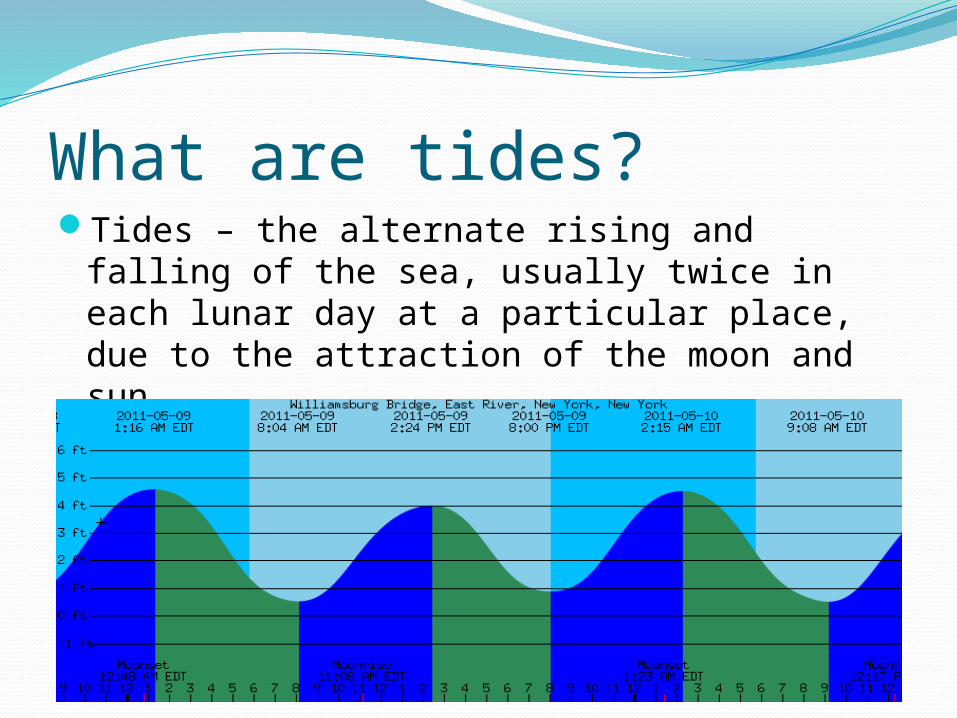
What are tides?Tides – the alternate rising and falling of the

sea, usually twice in each lunar day at a particular place, due to the attraction of the moon and sun

Currents generated by tides

TidesFlood tide – tide propagates onshore

High tide – water level reaches highest point

Ebb tide – tide moves out to sea

Low tide – water level reaches lowest point

Slack tide – period of reversing wave (low

current velocity)

The East RiverNot a river

A tidal strait connecting the Atlantic Ocean to

the Long Island Sound

Semidiurnal tides

Flow of the river

What makes up velocity

Direction

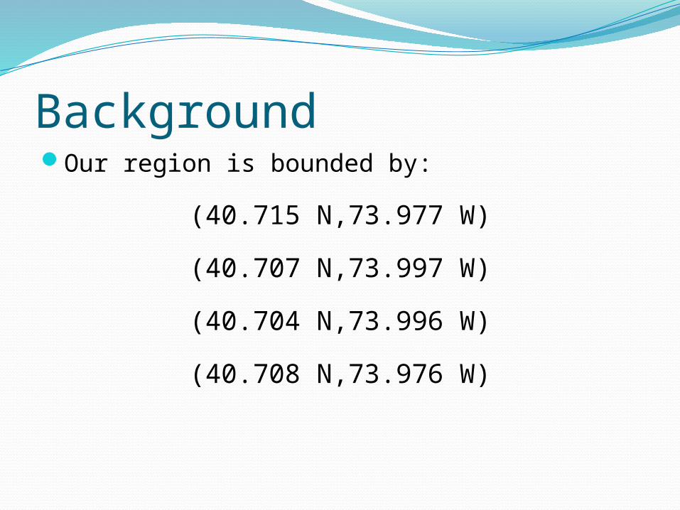
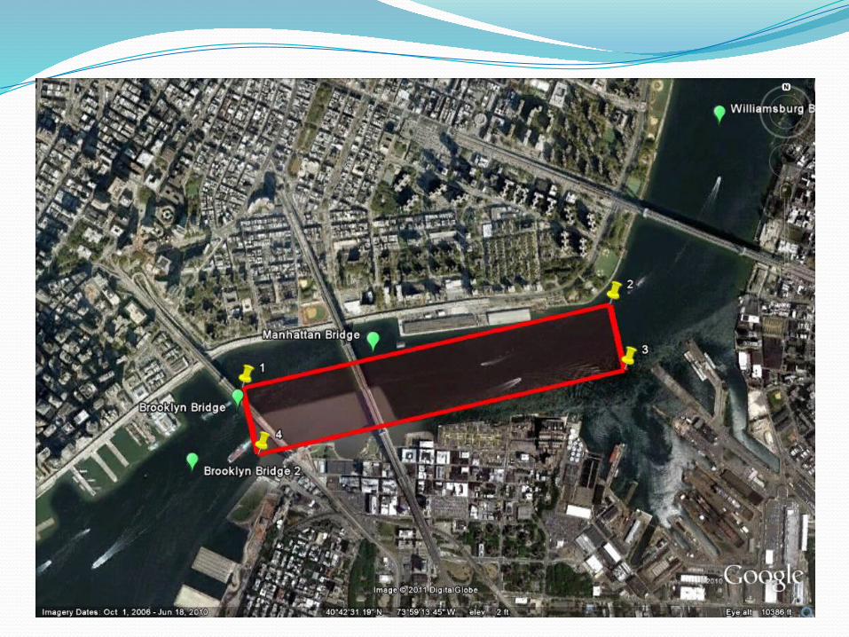
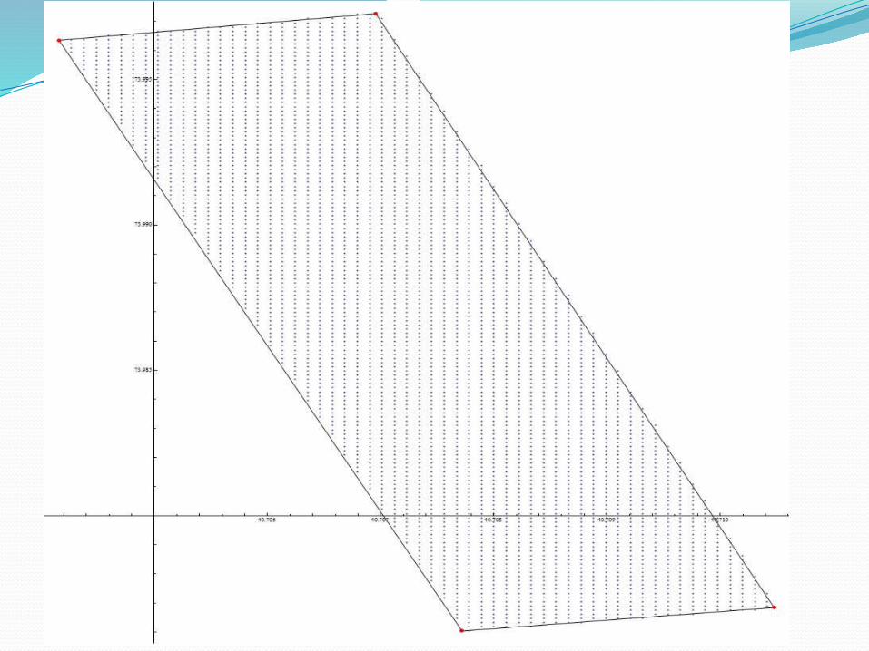
BackgroundOur region is bounded by:

(40.715 N,73.977 W)

(40.707 N,73.997 W)

(40.704 N,73.996 W)

(40.708 N,73.976 W)

BackgroundVideo of Tidal Turbine

Size of turbine

Each turbine has a rotor diameter of 4 meters

Type of turbine

Modeled after turbines used by Verdant Power (2007)

Efficiency

We are looking at a turbine efficiency of around 40%

MethodologyData from the National Oceanic and

Atmospheric Administration (NOAA)

Tidal velocity

Daily

2007-2011

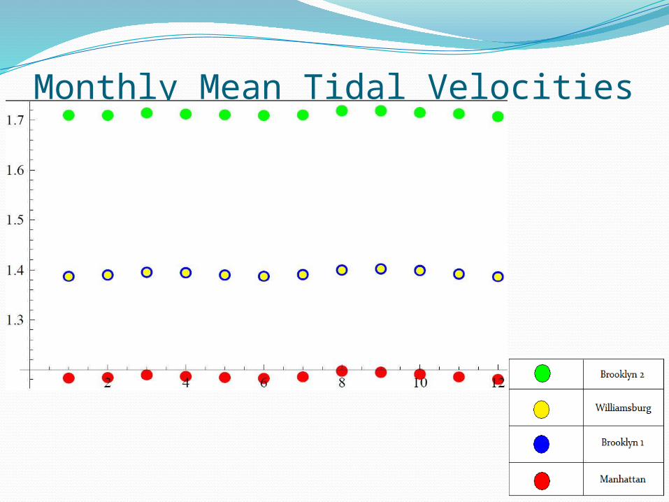
Monthly Mean Tidal Velocities

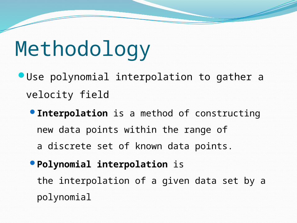
MethodologyUse polynomial interpolation to gather a

velocity field

Interpolation is a method of constructing new

data points within the range of a discrete set of

known data points.

Polynomial interpolation is the interpolation

of a given data set by a polynomial

Polynomial InterpolationSince we are working with four data points,

we need to find a third degree polynomial of

the form:

Thus, given any set of coordinates in our

region, (x,y), we can use this polynomial to

determine the velocity at that point

P(x,y) = a0+ a1 x+ a2y+ a3x2+ a4xy+ a5y2+ a6x3+ a7x2 y+ a8 x y2+ a9y3

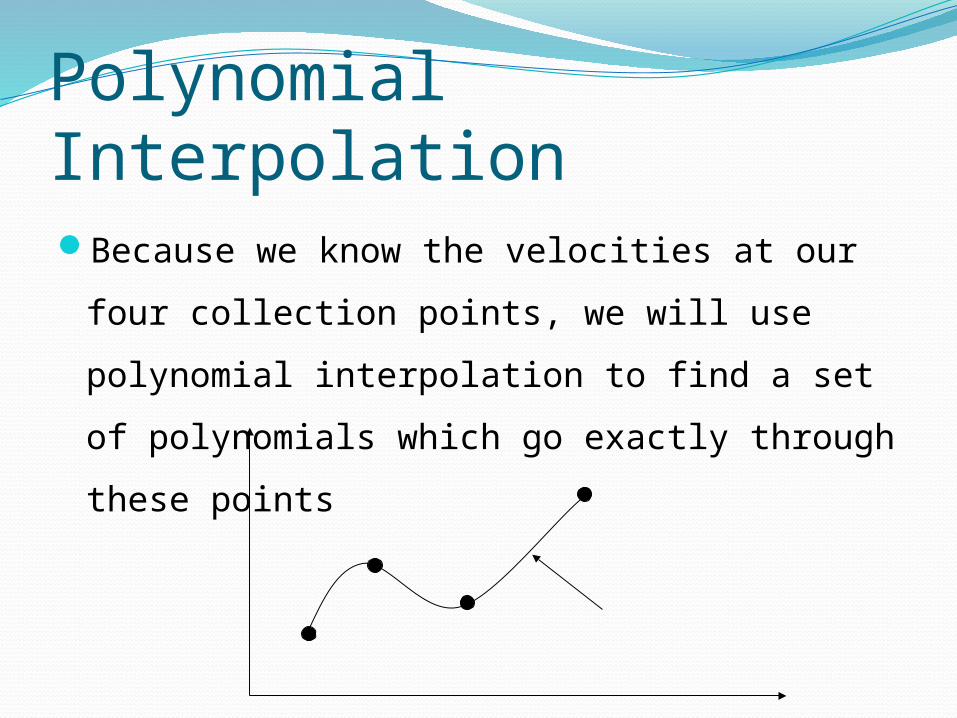
Polynomial InterpolationBecause we know the velocities at our four

collection points, we will use polynomial

interpolation to find a set of polynomials

which go exactly through these points

Polynomial Interpolation Begin by defining the matrix that will be

used to create our interpolating polynomials

The matrix is a 4 x 10 since there are 4 data points with coordinates and 10 terms in the polynomial that we are seeking

Polynomial InterpolationNow create a system of equations, so that we can solve

for the coefficients of our interpolating polynomials

Here is the average tidal velocity at

Polynomial InterpolationFinally, we have found our coefficients and

therefore our interpolating polynomials

Since we looked at the average tidal velocities

(mps) per month over the course of 5 years, we

have 12 separate polynomials (one for each

month)

We can use these polynomials to find the velocity

at any location in any month

Our PolynomialsP1[x,y] = 0.000299263 + 0.00984117 x + 0.362105 x2 + 15.4992 x3 + 0.0120129 y + 0.200942 x y + 0.679683 x2 y

+ 0.366569 y2 - 14.844 x y2 + 5.37202 y3

P2[x,y] = 0.000289367 + 0.00957213 x + 0.35658 x2 + 15.4945 x3 + 0.0115257 y + 0.191041 x y + 0.67966 x2 y +

0.348566 y2 - 14.8392 x y2 + 5.37048 y3

P3[x,y] = 0.000288423 + 0.00954475 x + 0.355857 x2 + 15.4786 x3 + 0.0114819 y + 0.190195 x y + 0.678976 x2 y

+ 0.347027 y2 - 14.8239 x y2 + 5.36498 y3

P4[x,y] = 0.000281853 + 0.00937133 x + 0.352788 x2 +15.5226 x3 + 0.01115 y + 0.183318 x y + 0.681046 x2 y +

0.334526 y2 - 14.8659 x y2 + 5.38031 y3

P5[x,y] = 0.00029242 + 0.00965699 x + 0.358498 x2 + 15.5127 x3 + 0.011673 y + 0.193988 x y + 0.680411 x2 y +

0.353925 y2 - 14.8568 x y2 + 5.37678 y3

P6[x,y] = 0.000297207 + 0.00978715 x + 0.361172 x2 + 15.5152 x3 + 0.0119087 y + 0.198776 x y + 0.680429 x2 y

+ 0.362631 y2 - 14.8593 x y2 + 5.37758 y3

P7[x,y] = 0.00029066 + 0.00960398 x + 0.356925 x2 + 15.4654 x3 + 0.0115946 y + 0.192525 x y + 0.678349 x2 y

+ 0.351262 y2 - 14.8114 x y2 + 5.36038 y3

P8[x,y] = 0.00029513 + 0.00971291 x + 0.35798 x2 + 15.3541 x3 + 0.0118348 y + 0.197724 x y + 0.673347 x2 y +

0.360707 y2 - 14.7051 x y2 + 5.32176 y3

P9[x,y] = 0.000282421 + 0.00938159 x + 0.352511 x2 + 15.4761 x3 + 0.0111863 y + 0.184186 x y + 0.67898 x2 y +

0.336101 y2 - 14.8214 x y2 + 5.36418 y3

P10[x,y] = 0.000279165 + 0.00929402 x + 0.350803 x2 + 15.4833 x3 + 0.0110244 y + 0.180872 x y + 0.679356 x2

y + 0.330076 y2 - 14.8281 x y2 + 5.36669 y3

P11[x,y] = 0.000291449 + 0.00963447 x + 0.358401 x2 + 15.5473 x3 + 0.0116189 y + 0.19279 x y + 0.681959 x2 y

+ 0.351751 y2 - 14.8898 x y2 + 5.38879 y3

P12[x,y] = 0.000292155 + 0.00965048 x + 0.358429 x2 + 15.5188 x3 + 0.0116588 y + 0.193682 x y + 0.680686 x2

y + 0.35337 y2 - 14.8626 x y2 + 5.37891 y3

Polynomial InterpolationOur polynomials appear similar which is due

to the fact the tidal velocities have minimal

seasonal change

This was verified when we plotted our contour

maps of the velocities and saw that they all

looked the same

Tidal Velocity Contour (mps)

Polynomial InterpolationPros

No error at the data pointsEasy to programAble to determine an interpolating polynomial just

given a set of points

ConsIt is only an approximationAccuracy dependent on the number of points you

interpolateNot the best technique for multivariate interpolation

Placement of the TurbinesEach Turbine needs to be approx. 9.8 – 24.4

meters (32-80 ft) apart (Verdant Power, 2007)

1 degree of latitude = 111047.863 meters

(364330.26 ft)

1 degree of longitude = 84515.306 meters

(277281.19 ft)

We decided to place the turbines 12.2 meters

(40 ft) apart

Placement of the TurbinesUsing Mathematica, given a min/max latitude

and longitude we were able find all points

that lie 40 feet apart from one another in a

set area

We then had to use basic mathematics to

confine the points to our particular area

Placement of the TurbinesUsing the fact that the

line thru pt1 and pt2 y = -5.80563 x + 310.327

line thru pt2 and pt3 y = 0.327377 x + 60.6708

line thru pt3 and pt4 y = -5.70626 x + 306.265

line thru pt4 and pt1 y = 0.292453 x + 62.0709

We used these lines to constrain the points to our

study area

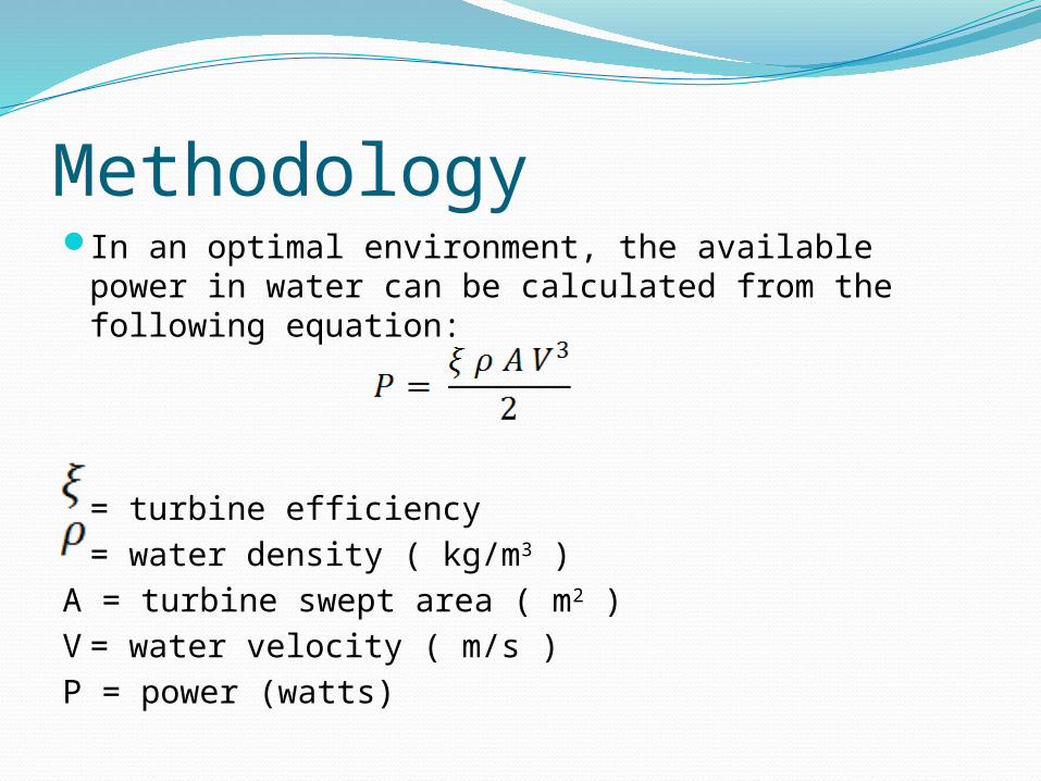
MethodologyIn an optimal environment, the available power in

water can be calculated from the following equation:

= turbine efficiency= water density ( kg/m3 )

A = turbine swept area ( m2 )V= water velocity ( m/s )P = power (watts)

FactsTotal number of homes in the Lower East

Side: 1546

On average, a household in America uses

10,000 kWh per year

Total energy needed: 15,460,000 kWh per

year

ResultsTotal number of turbines: 3794

Total energy from turbines: 21893.9 kWh

Total power output in a year: 1.91791 × 108

kWh

Total # of homes we could power in a year:

19179.1

DiscussionLimiting parameters

Velocity

Turbine efficiency

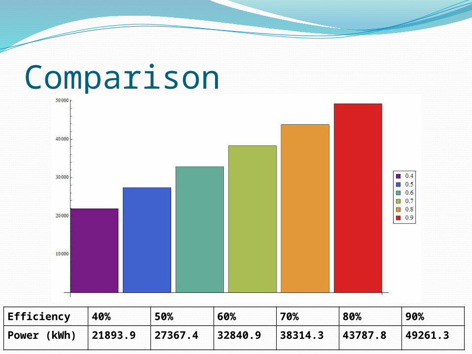
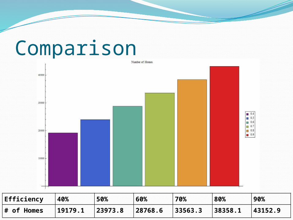
Comparison

Efficiency 40% 50% 60% 70% 80% 90%

Power (kWh) 21893.9 27367.4 32840.9 38314.3 43787.8 49261.3

Comparison

Efficiency 40% 50% 60% 70% 80% 90%

# of Homes 19179.1 23973.8 28768.6 33563.3 38358.1 43152.9

CostsThe turbines cost $2,000-$2,500 per kilowatt installed

Total Cost for 3794 turbines: 44 - 54 million dollars

Who pays:

In 2010, conEd gained a revenue of 25.8 ¢ per kWh to

residents and 20.4 ¢ per kWh for commercial and industrial.

The average yearly revenue for residencies alone would be

approximately 49 million dollars. conEd would start

profiting from the turbines in about a year after they are

installed.

BibliographyHardisty, Jack. "The Analysis of Tidal Stream Power." West

Sussex, UK: John Wiley & Sons, Ltd, 2009. 109-111.

NOAA. Tidal Current Predictions. 25 1 2011.

<http://tidesandcurrents.noaa.gov/curr_pred.html>.

Power, Verdant. The RITE Project.2007. 2011

<http://www.theriteproject.com/>.

Yun Seng Lim, Siong Lee Koh. "Analytical assessments on the

potential of harnessing tidal currents for electricity generation

in Malaysia." Renewable Energy (2010): 1024-1032.