Energy Flow Polynomials for Jet Substructure
42
Energy Flow Polynomials for Jet Substructure MIT Jet Workshop Cambridge, MA – January 11, 2018 Patrick T. Komiske III Center for Theoretical Physics, Massachusetts Institute of Technology PTK, E.M. Metodiev, J. Thaler – 1712.07124 Patrick T. Komiske III (MIT) EFPs for Jet Substructure 1 / 28
Transcript of Energy Flow Polynomials for Jet Substructure

Energy Flow Polynomials for Jet SubstructureMIT Jet Workshop
Cambridge, MA – January 11, 2018
Patrick T. Komiske IIICenter for Theoretical Physics, Massachusetts Institute of Technology
PTK, E.M. Metodiev, J. Thaler – 1712.07124
Patrick T. Komiske III (MIT) EFPs for Jet Substructure 1 / 28
Energy Flow Polynomials
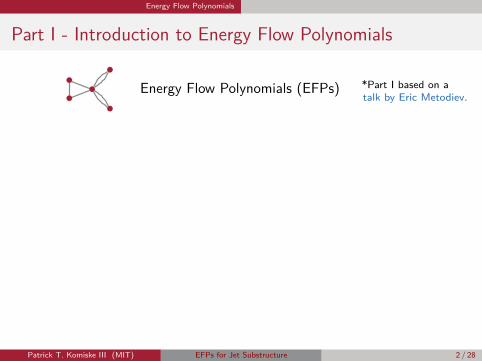
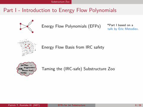
Part I - Introduction to Energy Flow Polynomials
Energy Flow Polynomials (EFPs)
Energy Flow Basis from IRC safety
Taming the (IRC-safe) Substructure Zoo
Spanning Substructure with Linear Regression
Patrick T. Komiske III (MIT) EFPs for Jet Substructure 2 / 28
*Part I based on atalk by Eric Metodiev.
Energy Flow Polynomials
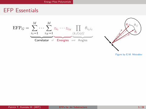
EFP Essentials
EFPG =M∑i1=1· · ·
M∑iN=1︸ ︷︷ ︸
Correlator
zi1 · · · ziN︸ ︷︷ ︸Energies
∏(k,`)∈G
θiki`︸ ︷︷ ︸Angles
e+e− measure: zi = Ei∑kEk
θij =(
2pµipjµ
EiEj
)β/2
Hadronic measure: zi = pT,i∑kpT,k
θij = (∆y2ij + ∆φ2
ij)β/2
e.g.
=M∑i1=1
M∑i2=1
M∑i3=1
M∑i4=1
zi1zi2zi3zi4θi1i2θi2i3θ2i2i4θi3i4
=M∑i1=1
M∑i2=1
M∑i3=1
M∑i4=1
M∑i5=1
zi1zi2zi3zi4zi5θi1i2θi2i3θi1i3θi1i4θi1i5θ2i4i5
Patrick T. Komiske III (MIT) EFPs for Jet Substructure 3 / 28
of and
Figure by E.M. Metodiev
“fly-swatter”
“bowtie”

Energy Flow Polynomials
Multigraph/EFP Correspondence
Multigraph ←→ EFP
j ←→ zijk ` ←→ θiki`
=M∑i1=1
M∑i2=1
M∑i3=1
M∑i4=1
zi1zi2zi3zi4θi1i2θi1i3θi1i4
N Number of vertices ←→ N -particle correlatord Number of edges ←→ Degree of angular monomialχ Treewidth + 1 ←→ Optimal VE Complexity
Connected ←→ PrimeDisconnected ←→ Composite
Patrick T. Komiske III (MIT) EFPs for Jet Substructure 4 / 28

EF Basis from IRC safety
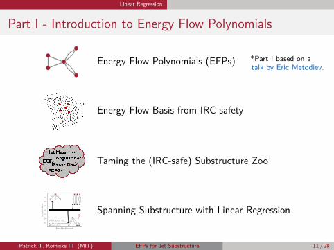
Part I - Introduction to Energy Flow Polynomials
Energy Flow Polynomials (EFPs)
Energy Flow Basis from IRC safety
Taming the (IRC-safe) Substructure Zoo
Spanning Substructure with Linear Regression
Patrick T. Komiske III (MIT) EFPs for Jet Substructure 5 / 28
*Part I based on atalk by Eric Metodiev.

EF Basis from IRC safety
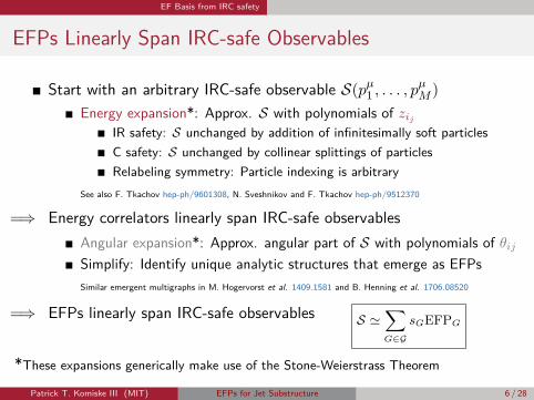
EFPs Linearly Span IRC-safe Observables
Start with an arbitrary IRC-safe observable S(pµ1 , . . . , pµM )
Energy expansion*: Approx. S with polynomials of zij
IR safety: S unchanged by addition of infinitesimally soft particlesC safety: S unchanged by collinear splittings of particlesRelabeling symmetry: Particle indexing is arbitrary
See also F. Tkachov hep-ph/9601308, N. Sveshnikov and F. Tkachov hep-ph/9512370
=⇒ Energy correlators linearly span IRC-safe observables
Angular expansion*: Approx. angular part of S with polynomials of θijSimplify: Identify unique analytic structures that emerge as EFPsSimilar emergent multigraphs in M. Hogervorst et al. 1409.1581 and B. Henning et al. 1706.08520
=⇒ EFPs linearly span IRC-safe observables
*These expansions generically make use of the Stone-Weierstrass Theorem
Patrick T. Komiske III (MIT) EFPs for Jet Substructure 6 / 28
S '∑G∈G
sGEFPG

EF Basis from IRC safety
EFPs Linearly Span IRC-safe Observables
Start with an arbitrary IRC-safe observable S(pµ1 , . . . , pµM )
Energy expansion*: Approx. S with polynomials of zijIR safety: S unchanged by addition of infinitesimally soft particlesC safety: S unchanged by collinear splittings of particlesRelabeling symmetry: Particle indexing is arbitrary
See also F. Tkachov hep-ph/9601308, N. Sveshnikov and F. Tkachov hep-ph/9512370
=⇒ Energy correlators linearly span IRC-safe observables
Angular expansion*: Approx. angular part of S with polynomials of θijSimplify: Identify unique analytic structures that emerge as EFPsSimilar emergent multigraphs in M. Hogervorst et al. 1409.1581 and B. Henning et al. 1706.08520
=⇒ EFPs linearly span IRC-safe observables
*These expansions generically make use of the Stone-Weierstrass Theorem
Patrick T. Komiske III (MIT) EFPs for Jet Substructure 6 / 28
S '∑G∈G
sGEFPG
EF Basis from IRC safety
EFPs Linearly Span IRC-safe Observables
Start with an arbitrary IRC-safe observable S(pµ1 , . . . , pµM )
Energy expansion*: Approx. S with polynomials of zijIR safety: S unchanged by addition of infinitesimally soft particlesC safety: S unchanged by collinear splittings of particlesRelabeling symmetry: Particle indexing is arbitrary
See also F. Tkachov hep-ph/9601308, N. Sveshnikov and F. Tkachov hep-ph/9512370
=⇒ Energy correlators linearly span IRC-safe observablesAngular expansion*: Approx. angular part of S with polynomials of θijSimplify: Identify unique analytic structures that emerge as EFPsSimilar emergent multigraphs in M. Hogervorst et al. 1409.1581 and B. Henning et al. 1706.08520
=⇒ EFPs linearly span IRC-safe observables
*These expansions generically make use of the Stone-Weierstrass Theorem
Patrick T. Komiske III (MIT) EFPs for Jet Substructure 6 / 28
S '∑G∈G
sGEFPG

EF Basis from IRC safety
Organization of the Energy Flow Basis
Need to select EFP subset GDetermine G by truncating in dFinite # of EFPs at each d
OEIS A050535:# of multigraphs with d edges# of EFPs of degree d
OEIS A076864:# of connect. multigraphs with d edges# of prime EFPs with degree d
Patrick T. Komiske III (MIT) EFPs for Jet Substructure 7 / 28
Substructure Zoo
Part I - Introduction to Energy Flow Polynomials
Energy Flow Polynomials (EFPs)
Energy Flow Basis from IRC safety
Taming the (IRC-safe) Substructure Zoo
Spanning Substructure with Linear Regression
Patrick T. Komiske III (MIT) EFPs for Jet Substructure 8 / 28
*Part I based on atalk by Eric Metodiev.

Substructure Zoo
Substructure Observables in the Energy Flow Context
Jet Mass: m2J
p2TJ
=M∑i1=1
M∑i2=1
zi1zi2(cosh(∆yi1i2)− cos(∆φi1i2)) = 12 × + · · ·
Angularities: λ(α) =M∑i=1
ziθαi
λ(4) = − 34 ×
λ(6) = − 32 × + 5
8 ×
Patrick T. Komiske III (MIT) EFPs for Jet Substructure 9 / 28
C.F. Berger, T. Kucs, and G. Sterman, hep-ph/0303051S.D. Ellis, et al., 1001.0014A.J. Larkoski, J. Thaler, and W. Waalewijn, 1408.3122
using pT -centroid axis
Substructure Zoo
Substructure Observables in the Energy Flow Context
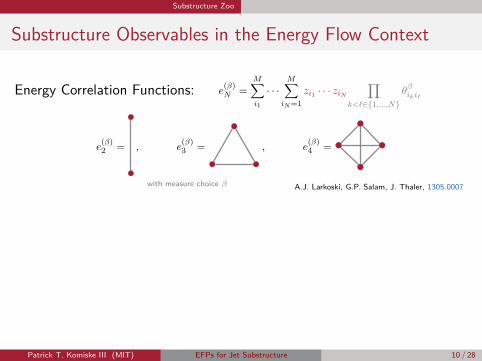
Energy Correlation Functions: e(β)N =
M∑i1
· · ·M∑
iN=1zi1 · · · ziN
∏k<`∈{1,...,N}
θβiki`
e(β)2 = , e
(β)3 = , e
(β)4 =
Geometric Moments: C =M∑i=1
zi
(∆y2
i ∆yi∆φi∆yi∆φi ∆φ2
i
), Pf = 4 detC
(TrC)2
Tr C = 12 × , 4 det C = − 1
2 ×
Patrick T. Komiske III (MIT) EFPs for Jet Substructure 10 / 28
A.J. Larkoski, G.P. Salam, J. Thaler, 1305.0007with measure choice β
L.G. Almeida, et al., 0807.0234 J. Thaler and Lian-Tao Wang, 0806.0023 J. Gallicchio and M. Schwartz, 1211.7038
using pT -centroid axis

Substructure Zoo
Substructure Observables in the Energy Flow Context
Energy Correlation Functions: e(β)N =
M∑i1
· · ·M∑
iN=1zi1 · · · ziN
∏k<`∈{1,...,N}
θβiki`
e(β)2 = , e
(β)3 = , e
(β)4 =
Geometric Moments: C =M∑i=1
zi
(∆y2
i ∆yi∆φi∆yi∆φi ∆φ2
i
), Pf = 4 detC
(TrC)2
Tr C = 12 × , 4 det C = − 1
2 ×
Patrick T. Komiske III (MIT) EFPs for Jet Substructure 10 / 28
A.J. Larkoski, G.P. Salam, J. Thaler, 1305.0007with measure choice β
L.G. Almeida, et al., 0807.0234 J. Thaler and Lian-Tao Wang, 0806.0023 J. Gallicchio and M. Schwartz, 1211.7038
using pT -centroid axis
Linear Regression
Part I - Introduction to Energy Flow Polynomials
Energy Flow Polynomials (EFPs)
Energy Flow Basis from IRC safety
Taming the (IRC-safe) Substructure Zoo
Energy Flow Polynomials
-1.5
-1.0
-0.5
0.0
0.5
1.0
1.5
Lea
rned
Coeffi
cien
t
W Jets: Ang. α = 6
Pythia 8.226,√s = 13 TeV
R = 0.8, pT ∈ [500, 550] GeV
EFP β = 1, d ≤ 7
Spanning Substructure with Linear Regression
Patrick T. Komiske III (MIT) EFPs for Jet Substructure 11 / 28
*Part I based on atalk by Eric Metodiev.
Linear Regression
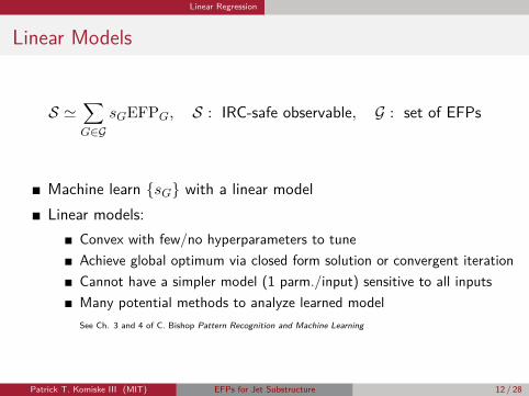
Linear Models
S '∑G∈G
sGEFPG, S : IRC-safe observable, G : set of EFPs
Machine learn {sG} with a linear modelLinear models:
Convex with few/no hyperparameters to tuneAchieve global optimum via closed form solution or convergent iterationCannot have a simpler model (1 parm./input) sensitive to all inputsMany potential methods to analyze learned modelSee Ch. 3 and 4 of C. Bishop Pattern Recognition and Machine Learning
Patrick T. Komiske III (MIT) EFPs for Jet Substructure 12 / 28
Linear Regression
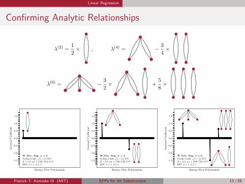
Confirming Analytic Relationships
λ(2) = 12 × , λ(4) = − 3
4 ×
λ(6) = − 32 × + 5
8 ×
Energy Flow Polynomials
-1.5
-1.0
-0.5
0.0
0.5
1.0
1.5
Lea
rned
Coeffi
cien
t
W Jets: Ang. α = 2
Pythia 8.226,√s = 13 TeV
R = 0.8, pT ∈ [500, 550] GeV
EFP β = 1, d ≤ 7
Energy Flow Polynomials
-1.5
-1.0
-0.5
0.0
0.5
1.0
1.5
Lea
rned
Coeffi
cien
t
W Jets: Ang. α = 4
Pythia 8.226,√s = 13 TeV
R = 0.8, pT ∈ [500, 550] GeV
EFP β = 1, d ≤ 7
Energy Flow Polynomials
-1.5
-1.0
-0.5
0.0
0.5
1.0
1.5
Lea
rned
Coeffi
cien
t
W Jets: Ang. α = 6
Pythia 8.226,√s = 13 TeV
R = 0.8, pT ∈ [500, 550] GeV
EFP β = 1, d ≤ 7
Patrick T. Komiske III (MIT) EFPs for Jet Substructure 13 / 28

Linear Regression
Linear Regression and IRC-safetymJ/pT,J : IRC safe - no Taylor expansion due to square rootλ(α=1/2): IRC safe - no simple analytic relationshipτ
(β=1)2 : IRC safe - algorithmically definedτ
(β=1)21 : Sudakov safe - safe for 2-prong jets and moreτ
(β=1)32 : Sudakov safe - safe for 3-prong jets and more
Multiplicity: IRC unsafe
2 3 4 5 6 7
Max Degree of EFPs
0.0
0.2
0.4
0.6
0.8
1.0
Cor
r.C
oef
.5
th−
95th
Per
centi
le
QCD Jets
Pythia 8.226,√s = 13 TeV
R = 0.8, pT ∈ [500, 550] GeV
EFP β = 1
mJ/pTJ
λ(α=1/2)
τ(β=1)2
τ(β=1)21
τ(β=1)32
Mult.
2 3 4 5 6 7
Max Degree of EFPs
0.0
0.2
0.4
0.6
0.8
1.0
Cor
r.C
oef
.5
th−
95th
Per
centi
le
W Jets
Pythia 8.226,√s = 13 TeV
R = 0.8, pT ∈ [500, 550] GeV
EFP β = 1
mJ/pTJ
λ(α=1/2)
τ(β=1)2
τ(β=1)21
τ(β=1)32
Mult.
2 3 4 5 6 7
Max Degree of EFPs
0.0
0.2
0.4
0.6
0.8
1.0
Cor
r.C
oef
.5
th−
95th
Per
centi
le
Top Jets
Pythia 8.226,√s = 13 TeV
R = 0.8, pT ∈ [500, 550] GeV
EFP β = 1
mJ/pTJ
λ(α=1/2)
τ(β=1)2
τ(β=1)21
τ(β=1)32
Mult.
Patrick T. Komiske III (MIT) EFPs for Jet Substructure 14 / 28
Conclusions
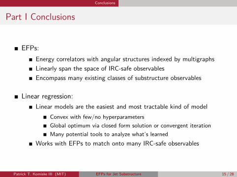
Part I Conclusions
EFPs:Energy correlators with angular structures indexed by multigraphsLinearly span the space of IRC-safe observablesEncompass many existing classes of substructure observables
Linear regression:Linear models are the easiest and most tractable kind of model
Convex with few/no hyperparametersGlobal optimum via closed form solution or convergent iterationMany potential tools to analyze what’s learned
Works with EFPs to match onto many IRC-safe observables
Patrick T. Komiske III (MIT) EFPs for Jet Substructure 15 / 28

Part II - Linear Jet Tagging with EFPs
Linear Classification with EFPs
Comparison with Modern Machine Learning
Fast Computation of EFPs
Patrick T. Komiske III (MIT) EFPs for Jet Substructure 16 / 28

Linear Classification
Linear Classification Overview
Fit a decision plane, determined by a vector w
Fisher’s linear discriminant (LDA): closed-form solutionLogistic regression: Convex, iterative solution
Decision threshold t is determined by distance from the planeG is finite set of graphs corresponding to the inputs
Organization by d is natural (equivalent to the order of the expansion)Organization by N or χ also possible, (where is the information?)
Classifier =
t+
∑G∈G
wGEFPG
≥ 0, signal< 0, background
Patrick T. Komiske III (MIT) EFPs for Jet Substructure 17 / 28

Linear Classification
Linear Classification with EFPs
W vs. QCD jet classification (quark/gluon and top tagging in backup)
0.0 0.2 0.4 0.6 0.8 1.0
W Jet Efficiency
10−1
100
101
102
103
Inve
rse
QC
DJet
Mis
tag
Rat
e
EFPs: W vs. QCD
Pythia 8.226,√s = 13 TeV
R = 0.8, pT ∈ [500, 550] GeV
EFP β = 0.5
d ≤ 3
d ≤ 6
d ≤ 7
Linear
DNN
better
300k training samplesLinear: Fisher’s linear discriminant
num. params. = num. EFPs < 1000100k test samples
DNN: Dense neural net(100 node fully-connected layer)× 3∼ 120k parameters50k validation, 50k test samples
Patrick T. Komiske III (MIT) EFPs for Jet Substructure 18 / 28
Linear Classification
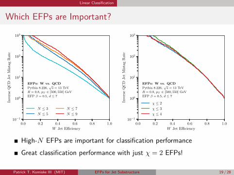
Which EFPs are Important?
0.0 0.2 0.4 0.6 0.8 1.0
W Jet Efficiency
10−1
100
101
102
103
Inve
rse
QC
DJet
Mis
tag
Rat
e
EFPs: W vs. QCD
Pythia 8.226,√s = 13 TeV
R = 0.8, pT ∈ [500, 550] GeV
EFP β = 0.5, d ≤ 7
N ≤ 3
N ≤ 5
N ≤ 7
N ≤ 9
0.0 0.2 0.4 0.6 0.8 1.0
W Jet Efficiency
10−1
100
101
102
103
Inve
rse
QC
DJet
Mis
tag
Rat
e
EFPs: W vs. QCD
Pythia 8.226,√s = 13 TeV
R = 0.8, pT ∈ [500, 550] GeV
EFP β = 0.5, d ≤ 7
χ ≤ 2
χ ≤ 3
χ ≤ 4
High-N EFPs are important for classification performance
Great classification performance with just χ = 2 EFPs!
Patrick T. Komiske III (MIT) EFPs for Jet Substructure 19 / 28
Modern ML Comparison
Part II - Linear Jet Tagging with EFPs
Linear Classification with EFPs
Comparison with Modern Machine Learning
Fast Computation of EFPs
Patrick T. Komiske III (MIT) EFPs for Jet Substructure 20 / 28
Modern ML Comparison
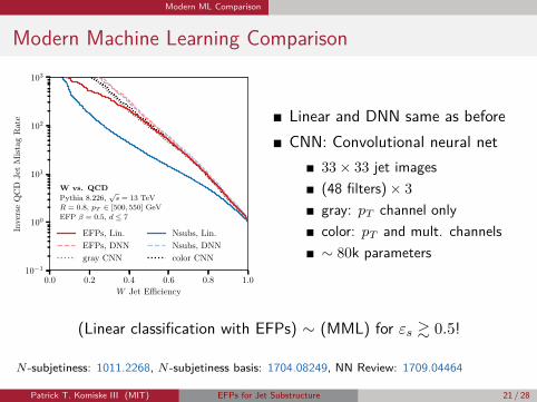
Modern Machine Learning Comparison
0.0 0.2 0.4 0.6 0.8 1.0
W Jet Efficiency
10−1
100
101
102
103
Inve
rse
QC
DJet
Mis
tag
Rat
e
W vs. QCD
Pythia 8.226,√s = 13 TeV
R = 0.8, pT ∈ [500, 550] GeV
EFP β = 0.5, d ≤ 7
EFPs, Lin.
EFPs, DNN
gray CNN
Nsubs, Lin.
Nsubs, DNN
color CNN
Linear and DNN same as beforeCNN: Convolutional neural net
33× 33 jet images(48 filters)× 3gray: pT channel onlycolor: pT and mult. channels∼ 80k parameters
(Linear classification with EFPs) ∼ (MML) for εs & 0.5!
N -subjetiness: 1011.2268, N -subjetiness basis: 1704.08249, NN Review: 1709.04464
Patrick T. Komiske III (MIT) EFPs for Jet Substructure 21 / 28

Modern ML Comparison
Modern Machine Learning Comparison
0.0 0.2 0.4 0.6 0.8 1.0
Quark Jet Efficiency
10−1
100
101
102
103
Inve
rse
Glu
on
Jet
Mis
tag
Rat
e
Quark vs. Gluon
Pythia 8.226,√s = 13 TeV
R = 0.4, pT ∈ [500, 550] GeV
EFP β = 0.5, d ≤ 7
EFPs, Lin.
EFPs, DNN
gray CNN
Nsubs, Lin.
Nsubs, DNN
color CNN
0.0 0.2 0.4 0.6 0.8 1.0
Top Jet Efficiency
10−1
100
101
102
103
Inve
rse
QC
DJet
Mis
tag
Rate
Top vs. QCD
Pythia 8.226,√s = 13 TeV
R = 0.8, pT ∈ [500, 550] GeV
EFP β = 0.5, d ≤ 7
EFPs, Lin.
EFPs, DNN
gray CNN
Nsubs, Lin.
Nsubs, DNN
color CNN
(Linear classification with EFPs) & (MML) for εs & 0.5
Patrick T. Komiske III (MIT) EFPs for Jet Substructure 22 / 28

Computation
Part II - Linear Jet Tagging with EFPs
Linear Classification with EFPs
Comparison with Modern Machine Learning
Fast Computation of EFPs
Patrick T. Komiske III (MIT) EFPs for Jet Substructure 23 / 28
Computation
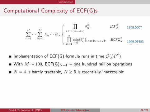
Computational Complexity of ECF(G)s
M∑i1=1· · ·
M∑iN=1
Ei1 · · ·EiN
∏i<j∈{i1,...,iN}
θβij , ECFβN
v∏m=1
min(m){θβij}i<j∈{i1,...,iN}, vECFGβN
Implementation of ECF(G) formula runs in time O(MN )
With M ∼ 100, ECF(G)N=4 ∼ one hundred million operations
N = 4 is barely tractable, N ≥ 5 is essentially inaccessible
fjcontrib – EnergyCorrelator 1.2.0
Patrick T. Komiske III (MIT) EFPs for Jet Substructure 24 / 28
1305.0007
1609.07483

Computation
Computational Complexity of ECF(G)s
M∑i1=1· · ·
M∑iN=1
Ei1 · · ·EiN
∏i<j∈{i1,...,iN}
θβij , ECFβN
v∏m=1
min(m){θβij}i<j∈{i1,...,iN}, vECFGβN
Implementation of ECF(G) formula runs in time O(MN )
With M ∼ 100, ECF(G)N=4 ∼ one hundred million operations
N = 4 is barely tractable, N ≥ 5 is essentially inaccessible
fjcontrib – EnergyCorrelator 1.2.0
Patrick T. Komiske III (MIT) EFPs for Jet Substructure 24 / 28
1305.0007
1609.07483
Computation
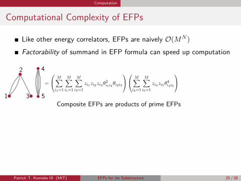
Computational Complexity of EFPs
Like other energy correlators, EFPs are naively O(MN )
Factorability of summand in EFP formula can speed up computation
=
M∑i1=1
M∑i1=1
M∑i3=1
zi1zi2zi3θ2i1i2θi2i3
M∑i4=1
M∑i5=1
zi4zi5θ4i4i5
=M∑i1=1
M∑i2=1
M∑i3=1
M∑i4=1
M∑i5=1
M∑i6=1
M∑i7=1
M∑i8=1
zi1zi2zi3zi4zi5zi6zi7zi8θi1i2θi1i3θi1i4θi1i5θi1i6θi1i7θi1i8︸ ︷︷ ︸O(M8)
=M∑i1=1
zi1
M∑i2=1
zi2θi1i2
7
︸ ︷︷ ︸O(M2)
Patrick T. Komiske III (MIT) EFPs for Jet Substructure 25 / 28
1
2
3
4
5Composite EFPs are products of prime EFPs

Computation
Variable Elimination (VE)
Algorithm for finding optimal parentheses placement in EFP formulaReduces EFP computational complexity to O(Mχ):
Best case (NP-hard): χ = treewidth(G) + 1Heuristics can be used which work excellently for our small graphsχ = 2 for all tree graphs, χ = 3 for single-cycle graphs, χ = N for KN
χ 2 3 4
e.g.
Patrick T. Komiske III (MIT) EFPs for Jet Substructure 26 / 28
Computation
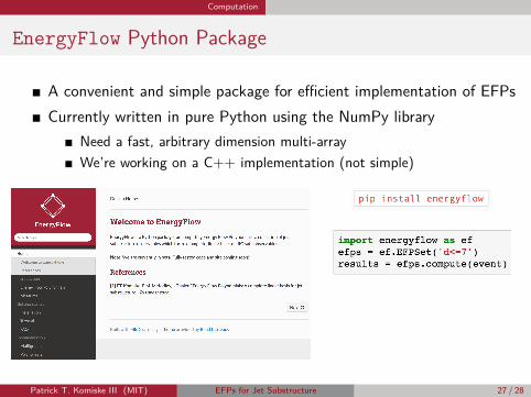
EnergyFlow Python Package
A convenient and simple package for efficient implementation of EFPsCurrently written in pure Python using the NumPy library
Need a fast, arbitrary dimension multi-arrayWe’re working on a C++ implementation (not simple)
Patrick T. Komiske III (MIT) EFPs for Jet Substructure 27 / 28
Conclusions
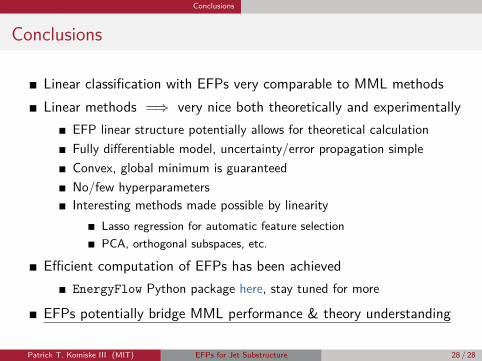
Conclusions
Linear classification with EFPs very comparable to MML methodsLinear methods =⇒ very nice both theoretically and experimentally
EFP linear structure potentially allows for theoretical calculationFully differentiable model, uncertainty/error propagation simpleConvex, global minimum is guaranteedNo/few hyperparametersInteresting methods made possible by linearity
Lasso regression for automatic feature selectionPCA, orthogonal subspaces, etc.
Efficient computation of EFPs has been achievedEnergyFlow Python package here, stay tuned for more
EFPs potentially bridge MML performance & theory understanding
Patrick T. Komiske III (MIT) EFPs for Jet Substructure 28 / 28

Backup
Additional Slides
Patrick T. Komiske III (MIT) EFPs for Jet Substructure 28 / 28
Backup
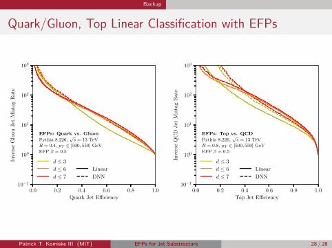
Quark/Gluon, Top Linear Classification with EFPs
0.0 0.2 0.4 0.6 0.8 1.0
Quark Jet Efficiency
10−1
100
101
102
103
Inve
rse
Glu
onJet
Mis
tag
Rat
e
EFPs: Quark vs. Gluon
Pythia 8.226,√s = 13 TeV
R = 0.4, pT ∈ [500, 550] GeV
EFP β = 0.5
d ≤ 3
d ≤ 6
d ≤ 7
Linear
DNN
0.0 0.2 0.4 0.6 0.8 1.0
Top Jet Efficiency
10−1
100
101
102
103
Inve
rse
QC
DJet
Mis
tag
Rat
e
EFPs: Top vs. QCD
Pythia 8.226,√s = 13 TeV
R = 0.8, pT ∈ [500, 550] GeV
EFP β = 0.5
d ≤ 3
d ≤ 6
d ≤ 7
Linear
DNN
Patrick T. Komiske III (MIT) EFPs for Jet Substructure 28 / 28
Backup
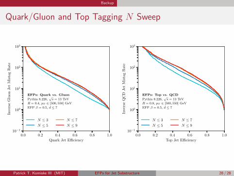
Quark/Gluon and Top Tagging N Sweep
0.0 0.2 0.4 0.6 0.8 1.0
Quark Jet Efficiency
10−1
100
101
102
103
Inve
rse
Glu
onJet
Mis
tag
Rat
e
EFPs: Quark vs. Gluon
Pythia 8.226,√s = 13 TeV
R = 0.4, pT ∈ [500, 550] GeV
EFP β = 0.5, d ≤ 7
N ≤ 3
N ≤ 5
N ≤ 7
N ≤ 9
0.0 0.2 0.4 0.6 0.8 1.0
Top Jet Efficiency
10−1
100
101
102
103
Inve
rse
QC
DJet
Mis
tag
Rat
e
EFPs: Top vs. QCD
Pythia 8.226,√s = 13 TeV
R = 0.8, pT ∈ [500, 550] GeV
EFP β = 0.5, d ≤ 7
N ≤ 3
N ≤ 5
N ≤ 7
N ≤ 9
Patrick T. Komiske III (MIT) EFPs for Jet Substructure 28 / 28

Backup
Quark/Gluon and Top Tagging χ Sweep
0.0 0.2 0.4 0.6 0.8 1.0
Quark Jet Efficiency
10−1
100
101
102
103
Inve
rse
Glu
onJet
Mis
tag
Rat
e
EFPs: Quark vs. Gluon
Pythia 8.226,√s = 13 TeV
R = 0.4, pT ∈ [500, 550] GeV
EFP β = 0.5, d ≤ 7
χ ≤ 2
χ ≤ 3
χ ≤ 4
0.0 0.2 0.4 0.6 0.8 1.0
Top Jet Efficiency
10−1
100
101
102
103
Inve
rse
QC
DJet
Mis
tag
Rat
e
EFPs: Top vs. QCD
Pythia 8.226,√s = 13 TeV
R = 0.8, pT ∈ [500, 550] GeV
EFP β = 0.5, d ≤ 7
χ ≤ 2
χ ≤ 3
χ ≤ 4
Patrick T. Komiske III (MIT) EFPs for Jet Substructure 28 / 28

Backup
N -Subjettiness Linear/DNN Comparison
0.0 0.2 0.4 0.6 0.8 1.0
Quark Jet Efficiency
10−1
100
101
102
103
Inve
rse
Glu
onJet
Mis
tag
Rat
e
Nsubs: Quark vs. Gluon
Pythia 8.226,√s = 13 TeV
R = 0.4, pT ∈ [500, 550] GeV
kT axes
2-body
6-body
10-body
Linear
DNN
0.0 0.2 0.4 0.6 0.8 1.0
W Jet Efficiency
10−1
100
101
102
103
Inve
rse
QC
DJet
Mis
tag
Rat
e
Nsubs: W vs. QCD
Pythia 8.226,√s = 13 TeV
R = 0.8, pT ∈ [500, 550] GeV
kT axes
2-body
6-body
10-body
Linear
DNN
0.0 0.2 0.4 0.6 0.8 1.0
Top Jet Efficiency
10−1
100
101
102
103
Inve
rse
QC
DJet
Mis
tag
Rat
e
Nsubs: Top vs. QCD
Pythia 8.226,√s = 13 TeV
R = 0.8, pT ∈ [500, 550] GeV
kT axes
2-body
6-body
10-body
Linear
DNN
Patrick T. Komiske III (MIT) EFPs for Jet Substructure 28 / 28
Backup
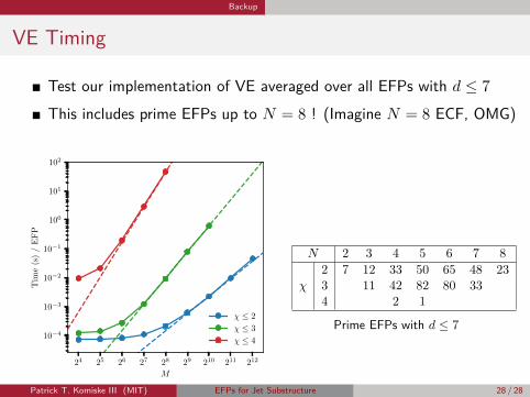
VE Timing
Test our implementation of VE averaged over all EFPs with d ≤ 7
This includes prime EFPs up to N = 8 ! (Imagine N = 8 ECF, OMG)
24 25 26 27 28 29 210 211 212
M
10−4
10−3
10−2
10−1
100
101
102
Tim
e(s
)/
EF
P
χ ≤ 2
χ ≤ 3
χ ≤ 4
N 2 3 4 5 6 7 82 7 12 33 50 65 48 23
χ 3 11 42 82 80 334 2 1
Prime EFPs with d ≤ 7
Patrick T. Komiske III (MIT) EFPs for Jet Substructure 28 / 28


![The Catchment Area of Jets - University of Arizonaatlas.physics.arizona.edu/~loch/material/papers...addressing issues such as jet substructure [2, 3, 4], the correlations between multi-jet](https://static.fdocuments.in/doc/165x107/60e2c799e02ccd0ce6163b2d/the-catchment-area-of-jets-university-of-lochmaterialpapers-addressing-issues.jpg)