
Energy Flow Analysis of an Academic Building › files › research › ... · Energy Flow Analysis...
105
Departement Meganiese en Megatroniese Ingenieurswese Department of Mechanical and Mechatronic Engineering Energy Flow Analysis of an Academic Building Marthinus Mynhardt Neethling 2011
Transcript of Energy Flow Analysis of an Academic Building › files › research › ... · Energy Flow Analysis...

Departement Megan iese en Megatron iese Ingen ieurswese
Department o f Mechanica l and Mechatronic Eng ineer ing
Energy Flow Analysis of an Academic
Building
Marthinus Mynhardt Neethling
2011
Departement Megan iese en Megatron iese Ingen ieurswese
Department o f Mechanica l and Mechatronic Eng ineer ing
Energy Flow Analysis of an Academic
Building
Marthinus Mynhardt Neethling
Master’s project presented in partial fulfilment of the requirements of the
degree Master of Engineering at Stellenbosch University
Supervisor: Prof. J. L. van Niekerk
December 2011

iii
DECLARATION
I, the undersigned, hereby declare that the work contained in this thesis is my own
original work and that I have not previously in its entirety or part submitted it at
any university for a degree.
Signature: ........................................................
M.M. Neethling
Date: 20/11/2011

iv
ABSTRACT
Increasing global concerns over the environmental impact of buildings have
stimulated the popularity of and need for energy-efficient buildings. This
realisation of the benefits that well-designed, so-called ‘green’ and energy-
efficient buildings provide, necessitated a standard for measuring such efficacy.
Various green building rating tools and national energy-efficient building
standards was therefore developed.
This study assesses the annual energy performance of a new academic building at
the University of Stellenbosch, Stellenbosch (South Africa), by using both the
Green Building Council of South Africa’s Green Star rating system and the SANS
204 national energy-efficiency building codes. The building evaluated will be
constructed on the University’s campus, adjacent to the Mechanical Engineering
building in the Engineering Complex.
A comparative analysis was done between the actual building and a notional
building built to SANS 204 specifications, as prescribed by the GSSA-PEB rating
tool. Both the actual and notional building models however incorporated a few
deviations from the GSSA-PEB rating tool to more accurately reflect the actual
operating conditions of the building and SANS 204 energy-efficient building
requirements. A quantitative physical modelling approach through the use of
EnergyPlus as the energy- and thermal load simulation engine was furthermore
utilised for these building energy simulation models.
The results indicate that the actual building is consuming 16.5% more energy
annually than the notional building. A Green Star rating on the first design stage
data is therefore not possible, as the GSSA-PEB energy conditional requirement is
not met.
The primary causes identified for this large difference in energy consumption are
the lighting and the HVAC system. The actual building was found to have a
62.9% higher lighting-power density than the notional building; and the VAV
HVAC system of the notional building was found to be significantly more
efficient that the fan-coil system of the actual building.
A parametric analysis of the actual building fabric and HVAC- and lighting
systems was furthermore done to investigate possible energy-consumption
improvement options. These results identified the significant impact that a
reduction in lighting density and a more efficient HVAC system can have on the
annual energy consumption of the building. A brief financial analysis on these
significant energy improvement options also proved it to be a worthwhile
investment. Further results showed the positive energy offset that may be
accomplished by increasing the thermal mass in the external walls.

v
On-site renewable energy generation, a reduction in installed lighting capacity;
and a more efficient HVAC system are recommended as the first vital steps in
reducing the energy consumption of the building; thus enabling it to become
eligible for a Green Star SA rating. In light of these recommendations was a solar
PV array designed for the new building as the most viable on-site renewable
energy generation option to reduce the carbon footprint of the building.
vi
OPSOMMING
Die gewildheid van energie-doeltreffende geboue kan toegeskryf word aan die
toenemende globale bewustheid rakende die impak van geboue op die omgewing.
As gevolg hiervan het die voordelige eienskappe wat sogenaamde ‘groen’ en
energie-doeltreffende geboue inhou, ʼn standaard vir die meet van hierdie geboue
genoodsaak. Groen-gebou graderingsmetodes en nasionale standaarde vir gebou
energie-doeltreffendheid was dus ontwikkel.
Dié studie maak gebruik van die Green Building Council of South Africa se
Green Star graderingssisteem en SANS 204 se nasionale energiestandaarde vir
geboue om die jaarlikse energiegebruik van ʼn nuwe akademiese gebou te
beoordeel. Die gebou wat geëvalueer is, gaan gebou word op die kampus van die
Universiteit van Stellenbosch, Stellenbosch (Suid-Afrika), langs die bestaande
Meganiese Ingenieurswese-gebou in die Ingenieurswese geboue kompleks.
ʼn Vergelyking studie op die jaarlikse energie verbruik is gedoen tussen die
werklike- en ʼn verwysings gebou, wat “gebou” is volgens SANS 204 standaarde
soos voorgeskryf deur die GSSA-PEB graderings instrument. Beide die modelle
van die werklike- en verwysingsgebou het ʼn paar afwykings van die GSSA-PEB
instrument ingesluit om die werklike bedryfs-kondisies van die gebou en SANS
204 se vereistes meer akkuraat te weerspieël. Dié gebou-energie simulasiemodelle
was gemodelleer deur ʼn kwantitatiewe model metode wat gebaseer is op die
fisiese eienskappe van die gebou. EnergyPlus was gekies as program vir die
simulasie van die gebou-energie en termiese lading.
Die resultate toon dat die werklike gebou jaarliks 16.5% meer energie verbruik as
die verwysingsgebou. Volgens die eerste ontwerpstekeninge is ’n Green Star-
gradering dus nie moontlik nie aangesien die primêre vereistes vir die GSSA-
energie kriteria nie nagekom is nie.
Die primêre oorsake van dié groot verskil in energie-verbruik is die beligtings- en
lugversorgingstelsels. Die werklike gebou toon ʼn 62.3% hoër beligtings-energie
digtheid as die verwysingsgebou; en daar was gevind dat die VAV lugversorging-
stelsel van die verwysingsgebou aansienlik meer doeltreffend is as die waaier-
spoel sisteem van die werklike gebou.
ʼn Parametriese studie is verder uitgevoer op die werklike gebou se konstruksie en
beligtings- en lugversorgingstelsels om moontlike energie-besparing moontlik-
hede te ondersoek. Die resultate toon dat laer vlakke van beligtings-
energieverbruik en ʼn meer effektiewe lugversorgingstelsel ʼn baie groot impak op
die jaarlikse energieverbruik van die gebou kan bewerkstellig. ʼn Kort finansiële
analise het ook getoon dat hierdie groot energie-besparing moontlikhede ʼn goeie
belegging sal wees. Verdere resultate toon dat indien die termiese massa van die

vii
eksterne mure verhoog word, die jaarlikse energieverbruik noemenswaardig
verlaag kan word.
Om die jaarlikse energieverbruik van die geboue te verlaag en só in aanmerking te
kom vir ʼn Green Star SA-gradering, word aanbeveel dat die opwekking van
hernubare energie op die terrein; ʼn vermindering in beligtings-energie en ʼn meer
effektiewe lugversorgingstelsel prioriteit moet neem. Met inagneming van hierdie
aanbevelings was ʼn son-energie PV stelsel ontwerp as ʼn hernubare energie opsie
om die koolstofvoetspoor van die nuwe gebou te verminder.

viii
ACKNOWLEDGEMENTS
Firstly, to my wife, your continual love and support cannot be described in mere
words.
I would like to express my gratitude to Mr Francois Joubert for his unwavering
support and guidance throughout this project.
Further gratitude goes to Prof. J.L. van Niekerk for his excellent supervision and
guidance.
I would also like to thank the great team at CRSES for their input throughout my
degree.
Finally I would like to extend a warm thanks to my family for their unending
support.
ix
TABLE OF CONTENTS
Declaration .............................................................................................................. iii
Abstract ................................................................................................................... iv
Opsomming ............................................................................................................. vi
Acknowledgements ............................................................................................... viii
List of Figures ........................................................................................................ xii
List of Tables ........................................................................................................ xiv
Nomenclature ........................................................................................................ xvi
1. Introduction .................................................................................................... 1
1.1. Background ......................................................................................... 1
1.2. New Academic Building .................................................................... 2
1.3. Format of the Study ............................................................................ 4
2. Literature Study and Background Information .............................................. 5
2.1. Building Envelope Performance ......................................................... 5
2.2. Thermal Comfort ................................................................................ 6
2.3. Green Buildings .................................................................................. 7
2.4. Green Building Rating Tools .............................................................. 9
2.5. Green Star SA ................................................................................... 10
2.5.1. Green Star SA – Eligibility Criteria ................................. 11
2.5.2. Green Star SA – Energy Criteria ...................................... 12
2.5.3. Green Star SA – Greenhouse Gas Emissions Credit........ 12
2.6. National Standards ............................................................................ 13
2.7. Energy Flow Assessment in Buildings ............................................. 14
2.7.1. Multi-Objective Optimisation Methods ........................... 14
2.7.2. Quantitative Physical Property Modelling ....................... 15
2.7.2.1. EnergyPlus ......................................................... 16
2.7.2.2. DesignBuilder .................................................... 18
2.7.3. Building Fabric Energy Flow Fundamentals ................... 19
3. Building Modelling ...................................................................................... 22
3.1. Overview .......................................................................................... 22
x
3.2. General Building Modelling Data .................................................... 24
3.2.1. Software ........................................................................... 24
3.2.2. Weather ............................................................................ 24
3.2.3. Location ........................................................................... 25
3.2.4. Building Design ............................................................... 26
3.2.5. Building Operational Schedules ....................................... 27
3.3. Actual Building Modelling ............................................................... 28
3.3.1. Criteria ............................................................................. 28
3.3.2. Modelling Data ................................................................ 28
3.3.2.1. Construction ....................................................... 29
3.3.2.2. Building Electrical Loads ................................... 30
3.3.2.3. HVAC ................................................................ 32
3.4. Notional Building Modelling. .......................................................... 35
3.4.1. Criteria ............................................................................. 35
3.4.2. Modelling Data ................................................................ 36
3.4.2.1. Construction ....................................................... 36
3.4.2.2. Building Electrical Loads ................................... 39
3.4.2.3. HVAC ................................................................ 39
3.5. Simulation Data ................................................................................ 41
3.5.1. Simulation Methodology.................................................. 41
3.5.2. Simulation Results ........................................................... 43
4. Parametric analysis ....................................................................................... 51
4.1. Building Fabric ................................................................................. 51
4.1.1. External walls ................................................................... 51
4.1.2. Glazing ............................................................................. 52
4.1.3. Roof .................................................................................. 53
4.2. Lighting System Efficiency .............................................................. 54
4.3. HVAC System Efficiency ................................................................ 55
5. Conclusions .................................................................................................. 58
6. Recommendations and future work .............................................................. 60
References .............................................................................................................. 61

xi
Appendix A: Building Façade Orientation ............................................................ 67
Appendix B: Simulation Model Floor Plans.......................................................... 68
Appendix C: Actual Building Lighting Design ..................................................... 72
Appendix D: GSSA-PEB Area Classification for New Academic Building ......... 74
Appendix E: Building Occupancy and Equipment Zone Data .............................. 76
Appendix F: Actual Building HVAC Data ............................................................ 78
Appendix G: CRSES Building Zones .................................................................... 80
Appendix H: Open Plan Office 2 Simulation Results ........................................... 81
Appendix I: Solar Photovoltaic Roof array ........................................................... 85

xii
LIST OF FIGURES
Page
Figure 1: Three-dimensional representation of the actual building simulation
model. ...................................................................................................... 3
Figure 2: Typical building envelope effects. ........................................................... 5
Figure 3: Relationship between PMV and PPD. ...................................................... 7
Figure 4: Triple bottom line. .................................................................................... 8
Figure 5: Example of a green academic building. ................................................... 9
Figure 6: Green Star SA Rating System. ............................................................... 10
Figure 7: SANS 204 climatic zones. ...................................................................... 14
Figure 8: EnergyPlus diagrammatical representation. ........................................... 16
Figure 9: EnergyPlus Successive Substitution Iteration ........................................ 17
Figure 10: EnergyPlus User Interfaces .................................................................. 18
Figure 11: External wall heat flux balance. ........................................................... 19
Figure 12: Construction element material composition example. ......................... 20
Figure 13: Equivalent thermal resistance circuit of Figure 12. .............................. 21
Figure 14: High-level, quantitative physical building property-modelling
breakdown. ........................................................................................... 22
Figure 15: Cape Town International Airport IWEC weather data. ........................ 24
Figure 16: Academic building location. ................................................................ 26
Figure 17: GSSA-PEB cellular office weekday profile. ........................................ 27
Figure 18: Actual building HVAC operational performance. ............................... 34
Figure 19: Fan Coil unit. ........................................................................................ 35
Figure 20: 113° Façade glazing representation of the actual building and the
notional building. ................................................................................. 38
Figure 21: VAV air handling unit. ......................................................................... 40
Figure 22: Notional building chiller performance curve. ...................................... 41
Figure 23: Annual building internal heat gains comparison between the actual and
notional building. ................................................................................. 43
xiii
Figure 24: Annual building fabric winter performance comparison between the
actual and notional building. ................................................................ 44
Figure 25: Actual building Open Plan Office 2 summer design week PMV. ....... 45
Figure 26: Notional building Open Plan Office 2 summer design week PMV. .... 46
Figure 27: Actual building typical winter day hourly internal gains. .................... 47
Figure 28: Notional building typical winter day hourly internal gains. ................. 47
Figure 29: Energy consumption category comparison between the actual building
and the notional building ..................................................................... 48
Figure 30: Building façade glazing effect on annual energy consumption. .......... 52
Figure 31: Plan view of actual building with façade orientation indication. ......... 67
Figure 32: Floor 1 - Library. .................................................................................. 68
Figure 33: Three dimensional representation of floor 1. ....................................... 68
Figure 34: Floor 2 - Library. .................................................................................. 69
Figure 35: Three dimensional representation of floor 2. ....................................... 69
Figure 36: Floor 3 - Lecture halls. ......................................................................... 70
Figure 37: Three dimensional representation of floor 3. ....................................... 70
Figure 38: Floor 4 - MIH and CRSES. .................................................................. 71
Figure 39: Three dimensional representation of floor 4. ....................................... 71
Figure 40: Actual building Open Plan Office 2 zone wireframe representation. .. 81
Figure 41: Actual building Open Plan Office 2 summer design day internal gains.
............................................................................................................. 82
Figure 42: Actual building Open Plan Office 2 summer design day fabric and
ventilation performance results. ........................................................... 83
Figure 43: Actual building Open Plan Office 2 winter design temperature and heat
loss results. ........................................................................................... 84
Figure 44: Plan view of academic building with PV array on roof . ..................... 85
Figure 45: PV array monthly energy output. ......................................................... 86

xiv
LIST OF TABLES
Page
Table 1: Thermal sensation scale. ............................................................................ 6
Table 2: Green Star SA – ratings. .......................................................................... 11
Table 3: Site location details. ................................................................................. 25
Table 4: Characteristics of new academic building. .............................................. 26
Table 5: Deviations from Green Star SA parameters. ........................................... 28
Table 6: Actual building construction elements. ................................................... 29
Table 7: Assumptions for an office’s electrical equipment requirements. ........... 31
Table 8: HVAC system chiller properties. ............................................................. 33
Table 9: Notional building construction elements. ................................................ 36
Table 10: SANS 204 minimum glazing requirements. .......................................... 37
Table 11: Notional building window-to-wall percentage. ..................................... 38
Table 12: Notional building HVAC design parameters. ........................................ 39
Table 13: Simulation results data origination. ....................................................... 42
Table 14: Actual building’s energy performance evaluation. ................................ 49
Table 15: Actual building’s CRSES area energy performance evaluation. ........... 50
Table 16: Annual building energy performance in terms of external wall’s cavity-
filling material. ...................................................................................... 51
Table 17: Annual building energy consumption increase in terms of building
glazing type. ........................................................................................... 53
Table 18: Annual building energy performance in terms of roof insulation
properties. .............................................................................................. 54
Table 19: Cost summary of lighting system energy reduction. ............................. 55
Table 20: Annual building energy performance in terms of HVAC system
configuration. ......................................................................................... 56
Table 21: Cost implications for changing HVAC system designs ........................ 56
Table 22: Cost summary of HVAC system design change from fan-coil to VAV.
............................................................................................................... 57
xv
Table 23: Lighting design comparison between actual design and GSSA-PEB
rating tool specifications. ....................................................................... 72
Table 24: GSSA-PEB area classification for new academic building. .................. 74
Table 25: Occupancy and equipment data per zone. ............................................. 76
Table 26: Actual Building HVAC Data ................................................................. 78
Table 27: Building zones which CRSES is comprised of. .................................... 80
Table 28: PV array specifications. ......................................................................... 86
Table 29: PV array simulation results. ................................................................... 86

xvi
NOMENCLATURE
Abbreviations
A/C Air-conditioning
ANN Artificial Neural Network
ASHRAE American Society of Heating Refrigeration and Air-
conditioning Engineering
BESTEST International Energy Agency Building Energy Simulation
Test and Diagnostic Method
BLAST Building Load Analysis and System Thermodynamics
BREEAM Building Research Establishment Environmental
Assessment Method
CASBEE Comprehensive Assessment System for Building
Environmental Efficiency
CBD Central Business Park
CFD Computational Fluid Dynamics
COP Coefficient of Performance
CRSES Centre of Renewable and Sustainable Energy Studies
CTF Conduction Transfer Function
DCR Discount Rate
DHW Domestic Hot Water
DOE-2 US Department of Energy Building Energy Simulation
Program, Version 2
EER Electrical Efficiency Ratio
EPW EnergyPlus Weather data
ESKOM National Utility (Electricity Supply Commission)
GBCSA Green Building Counsel of South Africa
GFA Gross Floor Area
GHG Greenhouse Gas Emissions
GSSA Green Star South Africa

xvii
HVAC Heating Ventilation and Air-conditioning
IEA International Energy Agency
IWEC International Weather for Energy Calculation
LEED Leadership in Environmental Energy Design
masl Meters Above Sea Level
MIH Myriad International Holdings
NCDC National Climatic Data Centre
NPV Net Present Value
PEB Public and Education Building
PMV Predicted Mean Vote
PPD Percentage People Dissatisfied
PV Photovoltaic
SA South Africa
SABS South Africa Bureau of Standards
SANS South African National Standard
U.S. United States of America
VAV Variable Air Volume
World GBC World Green Building Council
Symbols
A Area
An Glazing element area
C Thermal capacitance
CA,B,C SANS204 energy constants
cp Specific heat capacity
Ea Annual energy consumption
EI Energy index
Fa Façade area
h Convection heat-transfer coefficient
hr Radiation heat-transfer coefficient
k Thermal conductivity

xviii
K Kelvin
L Thermal load on body
M Metabolic rate
m Mass
QDHW Domestic hot water heating energy
Q Heat energy
cond Conduction heat energy
conv Convection heat energy
lw Long-wave radiation heat energy
sw Short-wave radiation heat energy
Pe Elevator power rating
Rn Glazing element thermal resistance
Rcond Conduction thermal resistance
Rconv Convection thermal resistance
Rrad Radiation thermal resistance
RT Total thermal resistance
Sn Glazing element SHGC
SHn SANS204 cooling shading multiplier
SCn SANS204 heating shading multiplier
t Operational hours
Ts Surface temperature
T∞ Temperature of a moving fluid
Tsur Surrounding environment temperature
UF Usage factor
Greek Symbols
ε Surface emissivity
ηDHW Domestic hot water heating efficiency
σ Stefan-Boltzmann constant
ΔT Temperature difference

1
1. INTRODUCTION
1.1. Background
More than 90% of the average person’s life is spent in buildings. As a result do
building fabric, location and design choices have both direct and indirect
influences on an individual’s physical and mental health (Evans, 2003). It has, for
example been shown that proper lighting; layout and ventilation design in hospital
buildings improves the health- and reduces stress and fatigue levels of the staff
and patients (Ulrich, et al., 2004). Further studies showed that insufficient
exposure to daylight in buildings results in sadness, fatigue and in some severe
cases, depression (Evans, 2003). The impact of buildings on mental health can
furthermore lead to indirect environmental impacts, because a human’s state of
mind influences his/her interaction with the environment. A building’s ability to
provide a healthy and productive indoor environment is therefore crucial in
ensuring the wellbeing of its occupants.
The built environment however has one of the largest carbon footprints of any
industry and bears a significant environmental impact. (Gunnell, 2009) Buildings
are also the largest and fastest-growing contributors to global energy demand, a
fact that can be attributed predominantly to population and economic growth. The
desire for improved comfort levels as a direct outcome of economic growth
furthermore increases the impact of buildings on the demand for energy (Pérez-
Lombard, et al., 2009).
Growth in the building sector is predicted to expand by approximately 34% in the
next 20 years with an annual average growth rate of 1.5%. The leading cause
behind this increase is the rapid growth in economic development of developing
countries (IEA, 2006).
Most of the energy currently consumed by the global building sector has largely
negative environmental impacts. This is primarily due to a few factors, including:
Fossil fuel-dominated electricity-generation sector;
Carbon-intensive processes required to produce the various materials that
building is composed of;
Land use and the impact of buildings on forestry and agriculture; and
Oil-dominated transportation sector.
Approximately 40% of the total environmental burden of member countries of the
European Union, for instance, is attributable to the building sector (Rey, et al.,
2007). Carbon dioxide emissions from this sector are furthermore responsible for
approximately 20% of the global greenhouse gas emissions (GBCSA, 2008).
2
The operational energy of a building typically accounts for the most significant
portion of the primary energy used during the lifespan of the building. This figure
is greatly influenced by building type, climatic region, building fabric
performance and the expected lifetime of the building. Scheuer et al. (2003) for
example, conducted a life-cycle primary energy analysis on a newly-constructed
engineering building located on the University of Michigan’s campus. The study
showed that over a designed life-span of 75 years, the primary energy of the
operations phase will amount to 97.7% of the total primary energy consumed.
Energy-efficient designs can therefore have a significant impact on the total life-
cycle primary energy use and can as a result reduce the carbon footprint of the
building. The building sector has furthermore been identified as one of the most
cost-effective sectors for reducing energy consumption and its carbon footprint
(IEA, 2010).
The concept of green and energy-efficient buildings was subsequently developed
to pursue the critical balance between occupant comfort and environmental impact
of buildings. This balance in a building from a carbon emissions perspective can
be achieved by designing a building envelope that maximises the use of natural
resources; uses optimised building mechanical and electrical systems and ensures
the creation of a healthy productive indoor environment for its occupants.
The realisation of the benefits that well-designed, so-called ‘green’ and energy-
efficient buildings provide, resulted in the creation of various rating tools for
green buildings and national energy-efficient building standards to provide a
standard for measuring such efficacy. The primary focus of these tools and
standards is to standardise and measure the balance achieved between occupant
comfort and the environmental impact of buildings.
These green building rating tools are not directly designed to provide a cost
benefit; however, a full cost benefit analysis that assess the direct and indirect
benefits of green buildings would in most cases result in a good initial investment
(Muldavin, 2010). The attractiveness of these green building investments is
furthermore enhanced by considering the total life-cycle impact of buildings, the
looming energy and water crisis in South Africa and the imminent carbon tax
legislation for buildings.
1.2. New Academic Building
The building evaluated in this study is a new academic building (shown below in
Figure 1) that will be constructed at the University of Stellenbosch, Stellenbosch
(South Africa), adjacent to the Mechanical Engineering building on the
Engineering Campus. Completion of the entire building is scheduled for early
2012.

3
The University’s planning committee has attempted to incorporate various
energy-efficiency measures in the initial design of this building. This is partly
because it will be the new home of the Centre of Renewable and Sustainable
Energy Studies (CRSES), an engineering department that is naturally concerned
with the environmental impact of buildings.
Another building design consideration is the desire to be the first academic
building in South Africa to be considered for a Green Star SA (GSSA) rating,
which is discussed in more detail in Section 2.5 below. This accreditation can
serve as both an advertisement and statement to demonstrate the University’s
commitment to reduce its environmental impact. A detailed building energy-
simulation is therefore needed to assess the energy performance of the building by
comparing it to national energy-efficient building standards (SABS - SANS 204,
2008).
Figure 1: Three-dimensional representation of the actual building simulation
model.
This study was launched as a direct and natural outcome of the University’s
aspirations for the new building. The general aim of the study is to assess the
overall energy performance of the new academic building by using national
standards and internationally accepted energy-efficiency rating tools for
comparative assessments. Although each building’s energy footprint is unique,
this study also aims to provide more insight into typical energy consumption
patterns of a tertiary education building.
The first of the outcomes of this study is to undertake a comparative energy
performance assessment between the actual building and the same building built

4
according to minimum SANS 204 requirements (referred to as the notional
building), as interpreted by the GSSA Public and Educational Building (PEB)
rating tool (2011).
The second outcome of the study is to do a full analysis of the actual building
fabric and operational energy performance; and the effect that each of the largest
energy consuming elements has on the building’s overall and annual energy
consumption. The third and final outcome is the evaluation and proposal of
possible building fabric and operational energy-improvement options.
1.3. Format of the Study
This report is structured around five main parts. For the first part, chapters 1 and 2
document the background, concepts and theory associated with green buildings
and energy modelling.
Part two is covered in Section 3.1 to 3.4 and documents the background,
modelling data and processes involved in the creation of simulation models for
both buildings. This section also evaluates the collective and individual simulation
model properties of each building.
The third part covered in Section 3.5 consists of a discussion of the modelling and
simulation data of the actual and notional building. A comparative study is also
done in this section to determine the energy performance of the actual building,
evaluated against the notional building results.
In the fourth part, contained in chapter 4, a detailed parametric and possible
optimisation options study is done to determine which building fabric element or
system in the actual building can be changed to result in a lower annual energy
performance. This part also briefly evaluates the financial implications of the
largest energy performance improvement options.
In the final part, which is covered by chapters 5 and 6, conclusions are drawn
from the comparative and parametric analysis done on the actual building; and the
possible inclusion of a PV renewable energy generation system is evaluated.
Future work and recommendations are also discussed.

5
2. LITERATURE STUDY AND BACKGROUND INFORMATION
2.1. Building Envelope Performance
A building envelope may be regarded as an enclosed, artificially- or naturally-
controlled environment that is separated from the outdoor environment. The
building envelope provides thermal insulation for controlling the radiative,
convective and conductive heat gains or losses.
A well-designed building envelope reduces energy requirements for artificial
environmental control and maximises the use of natural energy sources to ensure
sufficient comfort levels for the building’s occupants (Sustaining the Legacy,
2010). A building envelope designed according to green building principles
should furthermore perform consistently well throughout its proposed lifespan
(Harris, 2010).
Typical effects influencing the indoor climate of a building envelope are shown
below in Figure 2. These effects need to be controlled in an enclosed environment
to ensure occupant comfort.
Figure 2: Typical building envelope effects (Harris, 2010).
Conventional energy-efficiency measures for building envelopes can have a
significant impact on the operational energy demand and carbon footprint of
buildings without compromising occupants’ health and wellbeing. These
measures typically include increasing the insulation of building materials;
changing the building’s glazing properties; and ensuring an optimum building
orientation.
Over a period of 10 years, Kneifel (2010) evaluated 576 scenarios on 12
prototypical buildings simulated in 16 different cities to determine the average
energy performance of these buildings. He concluded that conventional energy-

6
efficiency measures can reduce the energy consumed in new commercial
buildings by between 20% and 30% on average; whilst some scenarios even
achieved an energy reduction of 40%. Further advantages include an average
carbon footprint reduction of 16% and an increased return on investment.
2.2. Thermal Comfort
One of the most important features of a well-designed building in its operational
phase is the ability to provide thermally comfortable conditions for its occupants.
Thermal comfort as defined by ASHRAE (2004) is the “condition of the mind in
which satisfaction is expressed with the thermal environment”.
This means that thermal comfort cannot be reduced to a specific state condition,
but is subject to a varying level of thermal sensation perceived as a state of
comfort for each respective individual. Factors in the building environment that
affect thermal comfort of an individual include (Auliciems & Szokolay, 2007;
Djongyang, et al., 2010):
Air temperature;
Air velocity;
Humidity;
Radiant temperature;
Individual metabolic rate; and
Individual clothing insulation.
The indicator used for measuring the thermal comfort of the occupants in this
study is the PMV-PPD index. Predicted mean vote (PMV) is a concept that was
introduced by Fanger (1970) and represents the mean value of the thermal comfort
votes of a large group of people. To establish the level of thermal comfort
experienced, PMV index values are measured against the ASHRAE Standard 55
(2004).
Table 1: Thermal sensation scale (ASHRAE, 2004).
Value +3 +2 +1 0 -1 -2 -3
Sensation Hot Warm Slightly
warm Neutral
Slightly
cool Cool Cold
PMV is formulated as follows:
[ ] (1)
In equation (1) above is M the metabolic rate and L the thermal load on the body
of the occupant. This thermal load can be defined as the difference between the

7
internal heat production of an occupant at comfort temperature and the heat loss to
the environment as a result of sweating. (Fanger, 1970)
The predicted percentage of dissatisfied (PPD) people is an index that represents
the number of people who were dissatisfied with the thermal comfort index and is
formulated as follows:
(2)
Figure 3: Relationship between PMV and PPD (ASHRAE, 2004).
The ASHRAE (2004) standard for building comfort requirements allows PMV
values between -0.5 and +0.5 to be regarded as thermally comfortable for human
occupancy. These values enable a prediction that the amount of people who will
be dissatisfied with the thermal conditions, will range between five (5) and ten
(10) per cent (refer to Figure 3 above).
It should also be noted from Figure 3 that even if thermal neutrality is maintained,
there will always be dissatisfied people because of differences in perception of
thermal comfort.
2.3. Green Buildings
The concept of energy-efficient buildings dates as far back as 1851, when the
Crystal Palace in London (Great Britain) – a cast-iron and glass building
originally erected to house a major exhibition in Hyde Park – used passive
systems for improving the quality of the indoor environment. The decisive starting
point of the green building movement, however, may be traced to the early 1970s,
when a group of forward-thinking environmentalists, ecologists and architects
began to investigate the applicability of energy-efficient building principles.
World Earth Day in April 1970 and the 1973 OPEC oil embargo served as
catalysts to transform their efforts into the so-called green building movement
(USGBC, 2003).

8
A ‘green building’ is defined as an energy-efficient building created by using
environmentally-responsible and resource-efficient processes for the purpose of
minimising the total life-cycle environmental impact of a building. The key
elements of a green building are (U.S. Environmental Protection Agency, 2010;
GBCSA, 2008):
Energy efficiency;
Resource efficiency;
Minimal waste production and pollution;
Improving occupant productivity;
Improving occupant health; and
Protecting the natural environment.
Figure 4: Triple bottom line (Senmit, 2011).
The green building concept revolves around the triple bottom line approach of
sustainability, depicted in Figure 4 above. This approach denotes that a
sustainable future can only be realised by establishing a well-balanced scenario
between human comfort requirements, sound economic opportunities and
environment protection (Lützkendorf & Lorenz, 2005).
In green buildings, however, the emphasis is placed on determining how to attain
the best balance between people (social), the planet (environmental) and profit
(economic) to ensure a minimum negative environmental impact.
9
2.4. Green Building Rating Tools
Buildings are very complex structures with numerous subsystems, materials,
operations, and functions. These systems also have a high degree of interaction
with the outside environment (Rey, et al., 2007). The evaluation of the
performance of buildings is therefore a complex exercise if one wishes to obtain
realistic results (Horvat & Fazio, 2005).
To address these complexities, building rating tools like, for example, Green Star
SA (South Africa); LEED (USA); BREEAM (United Kingdom); and CASBEE
(Japan) have been developed. Each of these building rating tools addresses the
unique environmental concerns and imperatives for different building types and
their respective life-cycle phases in every diverse, designated region.
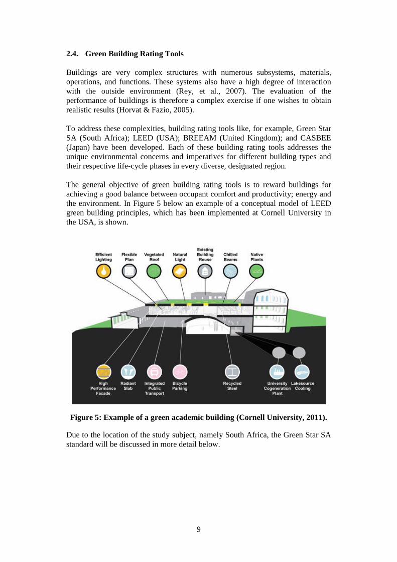
The general objective of green building rating tools is to reward buildings for
achieving a good balance between occupant comfort and productivity; energy and
the environment. In Figure 5 below an example of a conceptual model of LEED
green building principles, which has been implemented at Cornell University in
the USA, is shown.
Figure 5: Example of a green academic building (Cornell University, 2011).
Due to the location of the study subject, namely South Africa, the Green Star SA
standard will be discussed in more detail below.

10
2.5. Green Star SA
Green Star SA is a standard of measurement for green buildings located in South
Africa, and was introduced in 2008 by the Green Building Council of South
Africa (GBCSA), which is also a member of the World Green Building Council
(World GBC).
The relatively young South African Green Star rating system is based on the well-
established Australian Green Star rating model. This is mostly due to the
similarities in climate, building materials and general building practices between
the two countries. The Australian Green Star rating model is in turn derived from
the well-established LEED and BREEAM rating systems to ensure that global
experiences in the green building sector is utilised to the benefit of all.
A number of green building rating tools for different market sectors have been
released since the launch of the GSSA rating system. Currently available under
the GSSA canopy are the Office v1; Multi-Unit Residential v1; and the Retail
Centre v1 tools. The GSSA are also in the process of testing a future Public and
Educational Building rating tool. The main objectives of GSSA rating tools
include the provision of a standard of measurement for green buildings; the
recognition of environmental leadership; raising public awareness of green
buildings; encouraging integrated whole building design; and reducing the
environmental impact of buildings (GBCSA, 2008).
GSSA rating tools are divided into nine different categories that represent the
different environmental impacts of a building. Each of these categories is
subdivided into credits. The credits represent design initiatives that may improve
the environmental performance of a building. Points are awarded to each of these
credits to rate the level of achievement of the desired objective (GBCSA, 2008).
Figure 6: Green Star SA Rating System (GBCSA, 2008).

11
After a full assessment of all the credits in the each category, category scores are
calculated as percentages. Environmental weighting factors are then multiplied to
the score of each category as a representation of the different environmental
concerns and imperatives for building types and their respective life-cycle phases.
The final GSSA rating is then calculated as a sum of the scores of all the weighted
categories. A maximum possible value of 100 can be achieved for the sum of all
the weighted categories, excluding innovation. The latter is regarded as a way to
recognise and reward the use of innovative technologies and is therefore rewarded
over and above the maximum value of 100 for the other categories (GBCSA,
2008). The GSSA only awards market leaders in the field of green and efficient
buildings and will therefore only award and certify projects with four, five and six
star ratings, as shown below in Table 2.
Table 2: Green Star SA – ratings.
Score Rating Outcome
10-19 One star No certification
20-29 Two star No certification
30-44 Three star No certification
45-59 Four star Best practice
60-74 Five star South African excellence
75+ Six star World leadership
GSSA certification can be achieved in either “Design” or “As Built” format. A
building can be awarded a “Design” certification if it can be demonstrated that
sufficient green building principles have been incorporated in the building design
stage. The “As Built” certification can be awarded to a building that can verify the
implementation and procurement of green building principles.
2.5.1. Green Star SA – Eligibility Criteria
A building is only eligible for a GSSA rating if a series of eligibility criteria are
met. As the building assessed in this project is an educational building,
requirements for the GSSA Public and Educational Building (PEB) rating tool is
used. These criteria include spatial use and –differentiation; timing of
certification; and conditional requirements. The new academic building satisfies
both the spatial use and differentiation requirements as set forth in the GSSA –
Public & Education Building Pilot Eligibility Criteria document (GBCSA, 2011).
Conditional requirements in the PEB rating tool are the minimum required scores
for the ecology and energy categories that must be met to qualify for certification
regardless of other category scores (GBCSA, 2011). The ecology category’s

12
conditional requirement is not assessed in this study. For further information on
the energy conditional requirement, refer to Section 2.5.2 below.
2.5.2. Green Star SA – Energy Criteria
The main objective of the GSSA energy category is to minimise the overall
energy consumption of buildings and to encourage energy generation by
alternative sources.
A building’s total life-cycle carbon and other GHG emissions can be reduced
substantially by reducing the annual operational energy consumption of the
building. This is especially true in a South-African context where the energy
generation sector is dominated by coal-fired power plants. Another benefit of
reducing power consumption is to ease the load on the struggling electricity-
generating sector in South Africa and to thereby reduce the possibility of load-
shedding (GBCSA, 2008).
As mentioned in Section 2.5.1 above, the energy category is one of two categories
of the PEB rating tool that has a conditional requirement. In accordance with this
requirement, the actual building should perform equally to or better than a
notional building constructed to the ‘deemed-to-comply’ fabric- and building
service clauses of SANS 204:2008 Energy Efficiency in Buildings (SABS - SANS
204, 2008).
To demonstrate compliance to this criterion for a mechanically-ventilated
building, the following routes may be followed (GBCSA, 2008; GBCSA, 2011):
Compliance route 1: Energy modelling to show that the actual building
outperforms the notional building; or
Compliance route 2: Full compliance to the ASHRAE Advanced Energy
Design Guide for Small Office Buildings (ASHRAE, 2000) and a proven
HVAC energy consumption reduction of 20%; or
Compliance route 3: Full compliance to the SANS 204:2008 Energy
Efficiency in Buildings (SABS - SANS 204, 2008) ‘deemed-to-comply’
clauses.
The most important credit in the GSSA-PEB Energy category is the greenhouse
gas emissions credit. This credit’s purpose and relevance to this study is discussed
in further detail below.
2.5.3. Green Star SA – Greenhouse Gas Emissions Credit
The purpose of the energy credit is to reward greenhouse gas emission reductions
associated with the efficient operational energy consumption of buildings
(GBCSA, 2008).
13
Compliance to the credit criteria can be demonstrated by either following
compliance route 1 or 2, as discussed in Section 2.5.2 above. The academic
building examined in this project will however be evaluated in accordance with
compliance route 1. This route has been chosen because it requires a full
performance assessment of the annual energy requirements and awards the most
points for energy-efficient building design.
Compliance route 1 prescribes the awarding of points for the percentage of carbon
emission improvement of the actual building over the SANS 204 notional
building. This is done by comparing the energy modelling outcome of the actual
and notional building and translating the energy improvement to a reduction in
carbon emissions. Energy produced by on-site renewable energy sources,
however, is subtracted from the annual energy consumption of the actual building
before comparing it to the notional building energy consumption.
The relationship between energy efficiency and carbon emission reductions, as
used by the current GSSA–PEB V0 energy calculator, is 1.2 kg CO2/kWh
(ESKOM, 2007; GBCSA, 2011). Points are awarded on a linear scale with zero
(0) points for a carbon emission improvement of less than five (5) per cent over
the SANS 204 notional building and 20 points for a net zero emissions building
(GBCSA, 2008). Net zero emissions for a building is only achievable if all the
energy consumed annually by the building is produced by on-site renewable
energy sources.
2.6. National Standards
To demonstrate the energy- and environmental performance of the new academic
building evaluated in this study, compliance route 1 for the GSSA – PEB Energy
Criteria will be used as a guideline (refer to Section 2.5.3 for an explanation
hereof). Building performance will be evaluated against the ‘deemed-to-comply’
requirements of SANS 204:2008 Energy Efficiency in Buildings (SABS - SANS
204, 2008).
The objective of SANS 204 is to reduce energy consumption in buildings without
compromising the occupant’s comfort levels. Whereas compliance to this standard
is voluntary for new developments, the South African government will make the
‘deemed-to-comply’ SANS 204 requirements mandatory as soon as it is
economically viable for them to do so (Ashpole, 2009). The primary focus of this
standard is to improve heat-energy flows. This is done by changing the building
fabric according to the insulation properties specified for each climatic zone and
by reducing energy requirements of building systems (Reynolds, 2010).

14
The ‘deemed to satisfy’ thermal requirements of SANS 204 are based on six
designated climatic zones, as depicted in Figure 7. For each of these zones,
minimum thermal resistance R-values are specified for building fabric elements.
Figure 7: SANS 204 climatic zones (SABS - SANS 204, 2008).
2.7. Energy Flow Assessment in Buildings
The most common methods of forecasting building energy consumption include
prediction by multi-objective optimisation methods and simulation models based
on physical principles of buildings. Irrespective of which method is used for
forecasting energy consumption in buildings, there will always be some margin of
uncertainty. This can mainly be attributed to the fact that occupant behaviour is
near impossible to predict (Neto & Sanzovo, 2008) and global warming has
unknown effects on long-term weather patterns.
2.7.1. Multi-Objective Optimisation Methods
As a result of the non-linear nature of the input variables, gradient-free
optimisation methods are showing great promise for building energy prediction
(Magnier & Haghighat, 2009). When solving complex non-linear problems, the
most favourable method is the use of artificial neural networks (ANN) and

15
derivatives thereof (Li, et al., 2011; Yang, et al., 2005; Magnier & Haghighat,
2009; Ekici & Aksoy, 2007). ANN algorithms are based on mathematical models
used to simulate biological neural networks. These algorithms have the ability to
extrapolate results for new situations by investigating the underlying principle
governing previous situations (Neto & Sanzovo, 2008).
Due to ANN’s learning abilities, training is required to produce the desired set of
outputs and may be accomplished by providing the algorithm with data that
closely resembles desired output patterns. The data is then set up to identify
statistical patterns in the input parameters and to provide it with an intermediate
form of the previous two types of learning. The application of these ANN models
is therefore mostly based on previous measurements of existing models and not on
new developments.
Forecast applications of ANN building energy consumption suggest that very
accurate predictions can be achieved with relative ease compared to conventional
models based on physical principles (Cheng-wen & Jian, 2010; Ekici & Aksoy,
2007; Magnier & Haghighat, 2009; Wong, et al., 2008; Neto & Sanzovo, 2008).
The main disadvantage of forecasting building energy by such a complex
mathematical model is that it acts as a “black box”; thereby limiting the ability to
explicitly identify possible contributors to a particular output. Another
disadvantage includes that computational time of ANN models to converge to an
optimum may greatly exceed the computational time of physical models where a
large amount of input parameters is used (Tu, 1996).
Neural network optimisation algorithms are therefore more promising where the
optimisation of existing efficiency strategies is pursued (Neto & Sanzovo, 2008)
and as a quick and efficient tool to provide information on building energy
consumption at an early design stage (Cheng-wen & Jian, 2010). Physical models
are, however still the method of choice for applications when detailed, transparent
building energy simulation is needed.
2.7.2. Quantitative Physical Property Modelling
Models based on physical principles, like EnergyPlus, make use of prediction by
combing the physical properties of all foreseen energy sinks and sources; usage
profiles; uncertainties and the effect of external parameters (Neto & Sanzovo,
2008). These models typically require highly-detailed and -defined building
properties to obtain an accurate energy consumption prediction (Yezioro, et al.,
2007). The advantage of using highly defined input parameters includes the ability
to make detailed assessments to identify the level of contribution of each of the
energy consuming components. Building design and -operation can therefore be
optimised easily by exploring methods for reducing the energy consumption
contributions of each of its components.
16
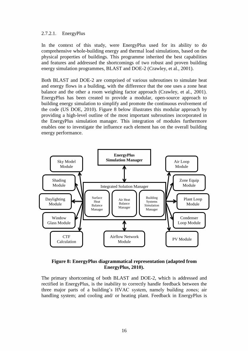
2.7.2.1. EnergyPlus
In the context of this study, were EnergyPlus used for its ability to do
comprehensive whole-building energy and thermal load simulations, based on the
physical properties of buildings. This programme inherited the best capabilities
and features and addressed the shortcomings of two robust and proven building
energy simulation programmes, BLAST and DOE-2 (Crawley, et al., 2001).
Both BLAST and DOE-2 are comprised of various subroutines to simulate heat
and energy flows in a building, with the difference that the one uses a zone heat
balance and the other a room weighing factor approach (Crawley, et al., 2001).
EnergyPlus has been created to provide a modular, open-source approach to
building energy simulation to simplify and promote the continuous evolvement of
the code (US DOE, 2010). Figure 8 below illustrates this modular approach by
providing a high-level outline of the most important subroutines incorporated in
the EnergyPlus simulation manager. This integration of modules furthermore
enables one to investigate the influence each element has on the overall building
energy performance.
Figure 8: EnergyPlus diagrammatical representation (adapted from
EnergyPlus, 2010).
The primary shortcoming of both BLAST and DOE-2, which is addressed and
rectified in EnergyPlus, is the inability to correctly handle feedback between the
three major parts of a building’s HVAC system, namely building zones; air
handling system; and cooling and/ or heating plant. Feedback in EnergyPlus is
EnergyPlus
Simulation Manager
Plant Loop
Module
Air Loop
Module
Zone Equip
Module
Condenser
Loop Module
PV Module Airflow Network
Module
Daylighting
Module
Sky Model
Module
Shading
Module
Window
Glass Module
CTF
Calculation
Integrated Solution Manager
Building
Systems Simulation
Manager
Air Heat
Balance
Manager
Surface
Heat Balance
Manager

17
accomplished by successive substitution iteration between the supply and demand
sides, as shown in Figure 9 below (EnergyPlus, 2010).
Figure 9: EnergyPlus Successive Substitution Iteration
The internal workings of EnergyPlus can be explained by dividing it into three
core components, namely a simulation manager; a building systems simulation
manager; and a heat- and mass balance module. The simulation manager acts as
an easily-controllable and modifiable module management shell wherein all the
major simulation loops and processes are contained. The building systems
simulation manager, however, controls the simulation of the systems, loads and
the HVAC plant of a building and then updates the zone-air conditions.
Air and surface heat- and mass balance modules form the core of the thermal
energy flow analysis of the EnergyPlus simulation engine. Both these modules are
controlled by the integrated solution manager (see Figure 8 above), which acts as
an interface between these modules and the building systems simulation manager.
A fundamental assumption underlying the air heat- and mass balance module is
that all air within each zone is assumed to be stirred well and maintained at a
uniform temperature. Assumptions for the surface heat- and mass balance module
include that zone surfaces, for example walls, windows, ceilings and floors, have
uniform surface temperatures; consistent long- and short wave radiation; diffuse
radiating surfaces and only one-dimensional heat conduction. Although these
assumptions do not reflect reality precisely, it provides a good and far less
computationally-intensive thermal assessment than using complex CFD models
for each zone (Crawley, et al., 2005).
The underlying principle of computing heat- and mass balance in these modules is
the application of the first law of thermodynamics between building element or air
interfaces and the control volumes around air masses in each zone. As heat
conduction in a building is time-dependent, transient heat conduction in these
heat-balance models are assessed using conduction-transfer functions (CTFs)
(Strand, et al., 1999). After the completion of a successful heat-balance simulation
in a time step, the building systems simulation manager is called to control the
simulation of the systems, loads and the HVAC plant to update the zone-air
conditions (Crawley, et al., 2005).
ZONE SYSTEM PLANT
Air Loop Water Loop

18
EnergyPlus has been comprehensively tested and validated by both the BESTEST
procedure (DesignBuilder, 2010), which was created by the IEA as an
accreditation tool for building energy simulation software. Further successful
testing and validation through the ASHRAE Standard 140-2001 procedure was
also accomplished (Crawley, et al., 2004). EnergyPlus is therefore the building
energy simulation programme of choice for the new academic building project
due to robust and proven performance and full compliance with the GSSA – PEB
energy modelling requirements (GBCSA, 2011).
2.7.2.2. DesignBuilder
DesignBuilder was selected for this study predominantly as a result of its ability
to provide a user-friendly, third-party graphical user interface for EnergyPlus.
Figure 10 below illustrates the high-level interaction between DesignBuilder and
EnergyPlus, where DesignBuilder is used as the third-party interface. This
interaction is limited to the creation of an input file and displaying of calculation
results.
Figure 10: EnergyPlus User Interfaces (Crawley, et al., 2005)
Other deciding factors for choosing DesignBuilder include the inclusion of a
three-dimensional, OpenGL geometric modeller; good visualisation capabilities;
well-defined graphical representation of building energy and environmental
performance data; and the ability to do building fabric performance comparisons.
A further advantage of using DesignBuilder as a user interface for EnergyPlus
above similar programmes like, for example, Sketchup-OpenStudio (Google,
2011) or Ecotect (Autodesk, 2011), is the availability of extensive data templates
for numerous building types. These fully-customisable templates provide a good

19
guideline that prescribes to what magnitude of input variable is typically expected
for certain building types.
2.7.3. Building Fabric Energy Flow Fundamentals
In the pursuit of understanding the factors influencing the rate and amount of
energy flows occurring through the building fabric, certain fundamental
thermodynamic principles should be discussed.
Energy flow characteristics of a building construction element can be defined in
terms of its thermal properties. Whenever a temperature gradient exists between a
construction element and its surrounding environment, heat energy is transferred.
Heat energy can be transferred in three different modes, namely conduction
through a solid or stationary fluid; convection between a surface and a moving
fluid; and radiation between two surfaces (Incropera & De Witt, 2002). In
Figure 11 below this heat-balance for a typical building construction surface is
demonstrated in terms of the rate of heat transfer per unit area normal to the
direction of heat transfer ( ) (Cengel, 2006).
Figure 11: External wall heat flux balance (adapted from EnergyPlus, 2010).
EnergyPlus calculates these energy flows by applying the first law of
thermodynamics to determine the heat flux balance in building elements
(EnergyPlus, 2010), as portrayed in equation (3):
(3)
The thermal conduction of the various elements in the building fabric is evaluated
in terms of equivalent thermal resistance R-value. This value is a measure of the
material’s ability to resist heat flow (q) across its thickness L in the direction
where there exists a temperature difference (Ts,1 - Ts,2) between surfaces. The
conduction R-value can be formulated as (Incropera & De Witt, 2002):
Convection where surface temperature
is less than outside temperature ( conv)
Long-wave radiation from
the environment ( lw)
Short-wave radiation, including direct,
reflected and diffuse solar radiation ( sw)
Conduction ( cond)
Wall
Reflected short-wave radiation ( sw-r)
Including
Emitted and reflected
long-wave radiation ( lw-r)

20
(4)
In equation (4), k is its thermal conductivity and A the area over which conduction
occurs. Similarly, as with conduction, an equivalent thermal resistance for heat
convection can be formulated (Incropera & De Witt, 2002) as follows:
(5)
In equation (5), T∞ is the temperature of the moving fluid and h the convection
heat-transfer coefficient.
Lastly, a thermal resistance equivalent for heat radiation can be formulated
(Incropera & De Witt, 2002) in accordance with equation (6) below:
(6)
In the equation above, Tsur is the temperature of the surrounding environment and
hr can be formulated, where reasonable assumptions for building loads are made
(Chapman, 1984), as (Incropera & De Witt, 2002):
(7)
where ε is the surface emissivity and σ the Stefan-Boltzmann constant.
There is an analogy between thermal resistance and electrical resistance, because
as thermal resistance is associated with heat conduction, electrical resistance is
associated with electricity conduction. These analogies make it possible for
thermal resistances to be modelled and calculated in the same manner as electric
resistive circuits (Incropera & De Witt, 2002). The equivalent thermal resistance
for a system can therefore be modelled and calculated as shown in Figure 12 and
Figure 13 below:
Figure 12: Construction element material composition example.
Radiation
( lw + sw)
Convection
( conv)
Material 3
Material 1
Material 2
Conduction
( cond)

21
Figure 13: Equivalent thermal resistance circuit of Figure 12.
The combined thermal resistance effects of heat conduction, convection and
radiation on the construction element shown in Figure 12 and Figure 13 are:
(8)
Another thermal energy flow property of building construction elements is the
ability to provide thermal capacitance, otherwise known as thermal mass. The
thermal energy storage ability of a material is determined by its mass and specific
heat capacity and is formulated as follows (Incropera & De Witt, 2002):
(9)
In equation (9), m is the mass of the object and cp is the specific heat constant of
the material. The heat energy stored in such an object can therefore be determined
by applying fundamental thermodynamic principles (Incropera & De Witt, 2002):
(10)
where q is the heat energy and ΔT the temperature difference across the object.
22
3. BUILDING MODELLING
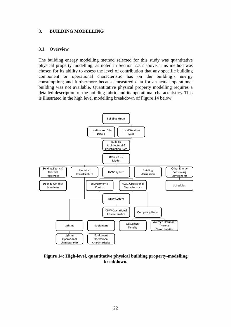
3.1. Overview
The building energy modelling method selected for this study was quantitative
physical property modelling, as noted in Section 2.7.2 above. This method was
chosen for its ability to assess the level of contribution that any specific building
component or operational characteristic has on the building’s energy
consumption; and furthermore because measured data for an actual operational
building was not available. Quantitative physical property modelling requires a
detailed description of the building fabric and its operational characteristics. This
is illustrated in the high level modelling breakdown of Figure 14 below.
Figure 14: High-level, quantitative physical building property-modelling
breakdown.

23
Building energy modelling can be done using a variety of methods. These range
from very accurate and complex, time-consuming models to basic, less accurate
and inexpensive models. This accuracy cost trade-off can usually be justified by
the predicted error margin resulting from the uncertainties of variables influencing
the energy consumption of the building model.
Uncertainties that have the largest impact on the energy consumption of academic
buildings are the following, listed in order of significance:
Occupancy density and –hours;
Occupants’ comfort perception and behaviour;
Weather patterns; and
Differences between the design version on which the modelling is based
and the completed physical building design.
Due to these uncertainties, approximations, for example, fixed occupancy density
and predefined occupancy schedules have to be made. The general method used
by the GSSA (2008) building energy rating system is to specify fixed occupant
comfort conditions, and schedules for occupancy and other energy consuming
components. This ensures that the building energy performance can be evaluated
with greater accuracy against reference models.
As the GSSA-PEB rating mechanism applicable to the building evaluated in this
study is only in pilot phase, the Green Star Office V1 tool was used as a reference
due to the similarities between the Office V1 and PEB Pilot rating tools. The
Energy Calculator & Modelling Protocol Guide - Version 0 (GBCSA, 2011) of
the GSSA-PEB Pilot tool was however used as a guideline for energy modelling.
These guidelines serve as an aid for pursuing accreditation when a full GSSA-
PEB rating study is conducted.
Another benefit of following these well-documented and internationally-
recognised guidelines is the ability to model and determine the applicability of
possible energy-saving initiatives between models with a fixed baseline. Each of
these initiatives can also be assessed to verify whether it will compromise
occupant comfort at the expense of saving energy.
Finally, these guidelines provide the ability to assess the energy performance of
the actual building measured against national standards. This is achieved by
comparing its energy performance to the same building built according to SANS
204 minimum energy-efficient building standards.

24
3.2. General Building Modelling Data
3.2.1. Software
As noted in Section 2.7.2.1 above, EnergyPlus was chosen as part of the
simulation package requirements of the GSSA–PEB Energy Calculator and
Modelling Protocol Guide (GBCSA, 2011). This simulation package passed both
the BESTEST and ANSI/ASHRAE Standard 140-2001 validation tests; of which
only one is required (GBCSA, 2011). DesignBuilder was furthermore used as a
graphical user interface to EnergyPlus. For both the actual and notional building,
were the energy flow simulations done with DesignBuilder version 3.0.0.48 and
EnergyPlus version 6.0.0.037.
3.2.2. Weather
The weather data used for energy flow modelling of the new academic building
was an international weather for energy calculation (IWEC) data file generated for
the Cape Town International Airport, Cape Town (South Africa). The new
academic building is located exactly 25.22 km in a straight line from the Cape
Town International Airport, and therefore fully conforms to the GSSA-PEB
(2011) requirements.
The IWEC weather file contains long-term typical weather data derived from up
to 18 years of historic hourly data acquired by the National Climatic Data Centre
(NCDC, 2011). A typical summer week of the weather data file used in the
academic building simulation models is depicted in Figure 15 below.
Figure 15: Cape Town International Airport IWEC weather data.

25
To simulate the effect that ground conditions have on the energy consumption of
the building, monthly temperatures provided by the IWEC weather data file was
used. This average monthly data is more than adequate for detailed building
simulation because ground temperatures vary slightly and slowly throughout the
year. A good rule of thumb for ground temperatures under large, conditioned
buildings is that it is 2°C less than the average monthly indoor space temperature
(DesignBuilder, 2010). The data used for this building was taken at a standard soil
diffusivity of 0.00232 m2/day and at a depth of 0.5 meter.
3.2.3. Location
The new academic building that forms the basis of this study will be situated at
the Stellenbosch University Engineering Campus, adjacent to the current
Mechanical Engineering building. The exact location details are depicted in
Table 3 below.
Table 3: Site location details.
Site attribute Value
Latitude 33°55’45.03” South
Longitude 18°51’57.34” East
Elevation above sea level 119.0 m
Site orientation (clockwise from true north) 23°
Building site type Greenfield
Building site footprint 1031.9 m2
Prevailing wind direction (clockwise from true north) 180°
From Figure 16 it is evident that both sunlight and wind will to a large extent be
restricted from this building due to the proximity of adjacent buildings. The new
building will however be ideally located between the main engineering
departments and will thus have the ability to make beneficial use of walkways and
to smoothly integrate with existing buildings.
Figure 31 in Appendix A shows a plan view of the academic building simulation
model and an indication of each façade orientation. This figure also demonstrates
that all the major buildings adjacent to the new academic building have been
incorporated into the simulation model. These buildings greatly influence the
external environment conditions, for example solar radiation and wind speed, of
the new building.

26
Figure 16: Academic building location (indicated by blue arrow) (adapted
from Google, 2011).
3.2.4. Building Design
This building will be used exclusively for academic purposes and will consist of
two levels of library space on the first and second floor; two lecture halls on the
third floor and the MIH media laboratory and CRSES on the fourth floor and
mezzanine.
The main spatial characteristics of the simulation model of the new academic
building are listed in Table 4 below. It is important to note that all these
characteristics were derived from the first architectural building design data and is
therefore subject to variation as minor changes may be implemented throughout
the construction and revision process.
Table 4: Characteristics of new academic building.
Spatial Characteristic Unit Value
Total building floor area (GFA) m2 3265
Total building volume m3 13754
Net conditioned building area m2 2709
Net conditioned building volume m3 11282
Unconditioned building area m2 555
External wall area m2 2967
External window glass area m2 544
External window–wall ratio: façade
on the 23° orientation % 7.8
N

27
External window–wall ratio: façade
on the 113° orientation % 39.4
External window–wall ratio: façade
on the 203° orientation % 30.1
External window–wall ratio: façade
on the 293° orientation % 5.1
3.2.5. Building Operational Schedules
Building operational schedules are nearly impossible to predict accurately. The
best method for evaluating the total building energy performance is therefore to
use fixed schedules that reflect the typical assumed operational profile of the
building.
In Appendix D of the GSSA–PEB Pilot v0 Energy Calculator & Modelling
Protocol Guide (2011), fixed schedules for the typical operational parameters
associated with an educational building are specified. The GSSA-PEB tool
provides a schedule for each general category generally found in an education
building. Each zone in the building has therefore been classified to fall under the
most relevant GSSA-PEB tool category.
The accuracy of the profiles used in the simulation models is not crucial as the
aim of the study is to assess the building energy performance and not to predict
the precise annual energy consumption. In Figure 17 below an example of one of
the profiles used in the simulation model, as prescribed by the GSSA-PEB tool, is
shown.
Figure 17: GSSA-PEB cellular office weekday profile.
0%
10%
20%
30%
40%
50%
60%
70%
80%
90%
100%
1 2 3 4 5 6 7 8 9 101112131415161718192021222324
Time (Hours)
Equipment
Lighting
Occupancy
HVAC
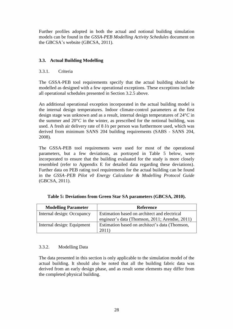
28
Further profiles adopted in both the actual and notional building simulation
models can be found in the GSSA-PEB Modelling Activity Schedules document on
the GBCSA’s website (GBCSA, 2011).
3.3. Actual Building Modelling
3.3.1. Criteria
The GSSA-PEB tool requirements specify that the actual building should be
modelled as designed with a few operational exceptions. These exceptions include
all operational schedules presented in Section 3.2.5 above.
An additional operational exception incorporated in the actual building model is
the internal design temperatures. Indoor climate-control parameters at the first
design stage was unknown and as a result, internal design temperatures of 24°C in
the summer and 20°C in the winter, as prescribed for the notional building, was
used. A fresh air delivery rate of 8 l/s per person was furthermore used, which was
derived from minimum SANS 204 building requirements (SABS - SANS 204,
2008).
The GSSA-PEB tool requirements were used for most of the operational
parameters, but a few deviations, as portrayed in Table 5 below, were
incorporated to ensure that the building evaluated for the study is more closely
resembled (refer to Appendix E for detailed data regarding these deviations).
Further data on PEB rating tool requirements for the actual building can be found
in the GSSA–PEB Pilot v0 Energy Calculator & Modelling Protocol Guide
(GBCSA, 2011).
Table 5: Deviations from Green Star SA parameters (GBCSA, 2010).
Modelling Parameter Reference
Internal design: Occupancy Estimation based on architect and electrical
engineer’s data (Thomson, 2011; Arendse, 2011)
Internal design: Equipment Estimation based on architect’s data (Thomson,
2011)
3.3.2. Modelling Data
The data presented in this section is only applicable to the simulation model of the
actual building. It should also be noted that all the building fabric data was
derived from an early design phase, and as result some elements may differ from
the completed physical building.

29
Only the most important aspects of the simulation model of the actual building are
discussed in this section. Further detailed information can be obtained by
contacting the author to examine the data file of the building’s simulation model.
3.3.2.1. Construction
Table 6 below gives a short description of the actual building’s construction
elements that are regarded by the GSSA-PEB Energy Modelling Protocol Guide
(2011) as the elements with the largest possible impact on the energy performance
of the building fabric. These construction elements are the roof, external walls and
windows.
Table 6: Actual building construction elements.
Construction
element
Thermal resistance
(m2K/W)
External surface
Characteristic Value
Roof1
4.6 Emissivity 0.90
Absorptivity 0.26
External walls2
1.01 Emissivity 0.94
Absorptivity 0.50
Single glazing
windows3 0.17 SHGF 0.78
Double glazing
windows3 0.37 SHGF 0.60
Notes: 1) Data acquired from ATI (2011) and the default DesignBuilder (2011) library. 2) Data
acquired from Corobrick (2009) and the default DesignBuilder (2011) library. 3) Data acquired
from the default DesignBuilder (2011) library.
At the time this study was conducted (2011), very limited information was
available on the shading devices or ‘blinds’ for the external windows. The only
windows where shading was incorporated into the design were the large windows
of the library on the 113°-façade; the large windows on each side of the lecture
halls; the large electronic classroom window; and the library window above the
large electronic classroom window.
Window shading control in the simulation model is managed by controlling the
amount of solar energy entering the room. All other external glazing was
modelled without window blinds due to the lack of available shading data.

30
3.3.2.2. Building Electrical Loads
Actual building electrical loads, excluding the electrical loads associated with the
HVAC system, can be subdivided into four categories: lighting, equipment,
domestic hot water (DHW) and elevator energy-usage.
All equipment and lighting loads simulated in the actual building model were the
actual design loads. These were obtained from the design data of the architect
(Thomson, 2011) and consulting electrical engineer (Arendse, 2011). All the
operational energy consumption levels were simulated according to the
operational schedules defined in Section 3.2.5 above.
The internal lighting density of the building was calculated as 15.51 W/m2 and the
total internal power rating for lighting as 55.06 kW. The power rating of external
lighting was also calculated as 1.07 kW (DesignBuilder, 2011; Arendse, 2011).
All internal lighting was modelled as suspended luminaries. The thermal effect of
these luminaries was modelled by dividing the lighting-energy into four fractions
that abide the following formula:
(11)
Where:
The return air fraction is zero (0), because no luminary ventilation is
provided;
A typical radiation fraction of 0.42 for fluorescent luminaries is assumed
(DesignBuilder, 2011);
A typical visible fraction of 0.18 for fluorescent luminaries is assumed
(DesignBuilder, 2011); and
The convective fraction is determined by Equation 11 above as 0.40.
The primary aim of the lighting system design was to provide robust, proven
technologies within a very limited budget. No intelligent lighting controls or LED
energy-efficient lighting products were therefore incorporated at the initial design
stage (Arendse, 2011). Further detailed lighting design data is given in Appendix
C, Table 23.
Electrical equipment loads were derived from architectural spatial usage data
(Thomson, 2011) and typical equipment power usage specifications, as consulted
with the University of Stellenbosch planning committee (refer to Appendix E,
Table 25). Some of the basic assumptions made for each person occupying an
office space are shown in Table 7 below. The total electrical equipment
(excluding the HVAC system and elevator) energy density of the building

31
measured over the GFA was calculated as 17.46 W/m2. To simulate the thermal
effect of this equipment, a radiant fraction of 0.2 was used (DesignBuilder, 2011).
Table 7: Assumptions for an office’s electrical equipment requirements.
(Whitehead, 2011)
Appliance Typical Wattage
Desktop Computer 400
Laptop Computer 100
Printers and Small Power 150
The GSSA-PEB rating tool specifies a very crude approximation of elevator
energy-use. Its annual energy consumption approximation for an elevator is based
on the assumption that the elevator operates for 75% of a 12-hour day for 365
days of the year. Due to the difficulty of predicting the actual operating profile of
the elevator, the GSSA-PEB rating tool approximation was used (GBCSA, 2011):
In Equation 12, Ea is the annual energy consumption, N is the number of
elevators, Pe is the elevator motor-power rating of each elevator, UF is the
prescribed 75% usage-factor and t is the number of operational hours per year.
Only one Kone 3000 P13 elevator (KONE, 2006) will be installed in the actual
building. The resulting annual energy consumption of the elevator, when
substituting the variables specified by the GSSA-PEB tool (2011) and the Kone
elevator specifications is therefore 19.05 MWh.
The domestic hot water (DHW) requirements for the building were calculated by
using the DHW specifications of the GSSA-PEB tool for each zone type (refer to
Appendix D). This amounted to a daily requirement of 424.4 l/day for the entire
building. The annual energy requirement Qeff for domestic hot water (DHW) was
thus calculated as follows:
(13)
In Equation 13, m is the mass of the water, cp is the specific heat capacity of
water, ΔT is the temperature difference between boiler water inlet- and outlet
temperature and ηDHW is the energy efficiency of the DHW system.
∑
(12)

32
In the calculation of annual DHW electricity power consumption, certain
assumptions have however been made, including:
Water inlet temperature is constant throughout the year at 15°C;
Supply water temperature is constant at 55°C;
Specific heat capacity (cp) of the water is constant at 4180 J/kg/K;
Efficiency of the whole DHW system is 95% due to the predominant use
of instant water heaters and geysers with very short distribution design
(Thomson, 2011);
One (1) kilogram of water is equal to one (1) litre of water; and
DHW is consumed 365 days of the year.
The water usage specifications per zone type (refer to Appendix D) set forth in
Appendix C of the GSSA–PEB Pilot v0 Energy Calculator & Modelling Protocol
Guide (2011) was used. The resulting annual DHW power consumption, in
accordance with the GSSA-PEB requirements, is 7.57 MWh.
3.3.2.3. HVAC
An HVAC system is typically one of the largest energy consuming components of
a mechanically air-conditioned building’s annual energy consumption (Al-Sanea,
et al., 2012).
The HVAC system to be implemented in the new academic building has two
chillers with a combined cooling capacity of 511 kW. Both units are connected to
a coolant storage tank from where the coolant is redistributed to the fan-coil air-
conditioning units in each zone (Meyer, 2011). The operational energy
consumption for each of these chillers is determined by the following three curves
(Hydeman & Gillespie, 1999; EnergyPlus, 2010) :
Cooling capacity as a function of evaporator and condenser temperatures;
Energy input to cooling output ratio as a function of evaporator and
condenser temperatures; and
Energy input to cooling output ratio as a function of percentage
unloading.
An accurate model for each chiller used in the new academic building (depicted in
Table 8 below) can be created by using linear regression techniques on a broad
range of measured performance data of each chiller. Hydeman et al. (1999)
developed a least-squares linear regression technique for calculating these curves
when adequate performance data is available.
Unfortunately performance data of the chillers used in the new academic building
could not be obtained from relevant suppliers. A further complication was that the
simulation model could only accommodate a single chiller unit. An equivalent

33
model for both chillers, that takes into account the effect of the storage tank and
interconnections, was therefore necessary.
Hydeman et al. (1999) tested chiller operational power characteristics against a
wide variety of well-documented models that are publicly available. The
researchers concluded that the DOE2 reference electric chiller model developed
by the U.S. Department of Energy provided the smallest RMS error at an average
of 1.8%. As a result Hydeman et al. recommend the use of a similar, well-
documented and -tested chiller model operating at reference conditions to be used
when insufficient operational data about the actual chillers is available (Hydeman
& Gillespie, 1999).
Table 8: HVAC system chiller properties (Meyer, 2011).
Chiller type Climaveneta NECS
/B 1614
Climaveneta NECS
-Q /B 0512
Cooling capacity 396 kW 115 kW (cooling
mode only)
Heating capacity - 136.5 kW (heating
mode only)
Cooling EER (at 100% load and
34°C inlet air temperature) 2.53 2.47
Heating EER (at 100% load) - 3.11
Cooling fluid pump power 11 kW 4 kW
Heating fluid pump power - 2.2 kW
Evaporator flow rate 68.2 m3/h 19.8 m
3/h
Heat recovery exchanger flow rate - 17.5 m3/h
A reference curve that best matched the specifications of the chillers to be
installed in the actual building was therefore used, as proposed by Hydeman et al.
(1999). The reference chiller chosen for this study, which best reflects the
characteristics of the chillers described in Table 8, was the DOE air-cooled chiller
model (DesignBuilder, 2011).
The heating- or cooling energy efficiency of each chiller is rated in terms of its
energy-efficiency ratio. This ratio indicates the heating or cooling energy
produced by the unit relative to the amount of electrical energy required to
generate it. The higher the EER, the more energy efficient the chiller unit will
therefore be. An approximated reference chiller EER, chosen to reflect the
combined EER of both chillers, was calculated by linear interpolation between the
known EER values at the same reference conditions of each chiller. This was done
by using the following formula:

34
(14)
In Equation 14, QChiller1 and QChiller2 are the cooling capacities of each chiller. This
is however a fairly simplistic approximation, as the true interconnected operation
of these chillers is unknown. Full operational EER versus normalised load for
both the actual building chillers are shown in Figure 18 below.
Figure 18: Actual building HVAC operational performance (Mienie, 2011).
The majority of the heating energy in the actual building will be provided by the
Climaveneta NECS –Q /B 0512 heat-recovery chiller and the rest by electric
elements. These elements were chosen as the best cost-effective method to
provide heating energy to the smaller zones on levels 1 and 2 (Meyer, 2011).
Further detailed information of the HVAC system to be installed in the actual
building is provided in Appendix F, Table 26.
The reference boiler EER for heating energy-consumption calculations in zones
where heating is provided by the NECS –Q chiller, is specified in Table 8 above.
Operational characteristics of the boiler were simulated by using a fixed EER of
3.11. The EER of all the electric elements in each zone was used as one (1), as
nearly all the electrical energy is converted into thermal energy.
Each zone utilises a simple fan-coil unit for air conditioning, as depicted in Figure
19 below (Meyer, 2011). A fan power consumption value of 2.1 W/l/s was used as
per SANS 204–3:2008 (2008) specifications. This value was chosen due to the
2.25
2.75
3.25
3.75
4.25
4.75
0.1 0.2 0.3 0.4 0.5 0.6 0.7 0.8 0.9 1
EER
Normalised Load
NECS /B: 20 deg C
NECS /B: 34 deg C
NECS -Q: 20 deg C
NECS -Q: 34 deg C
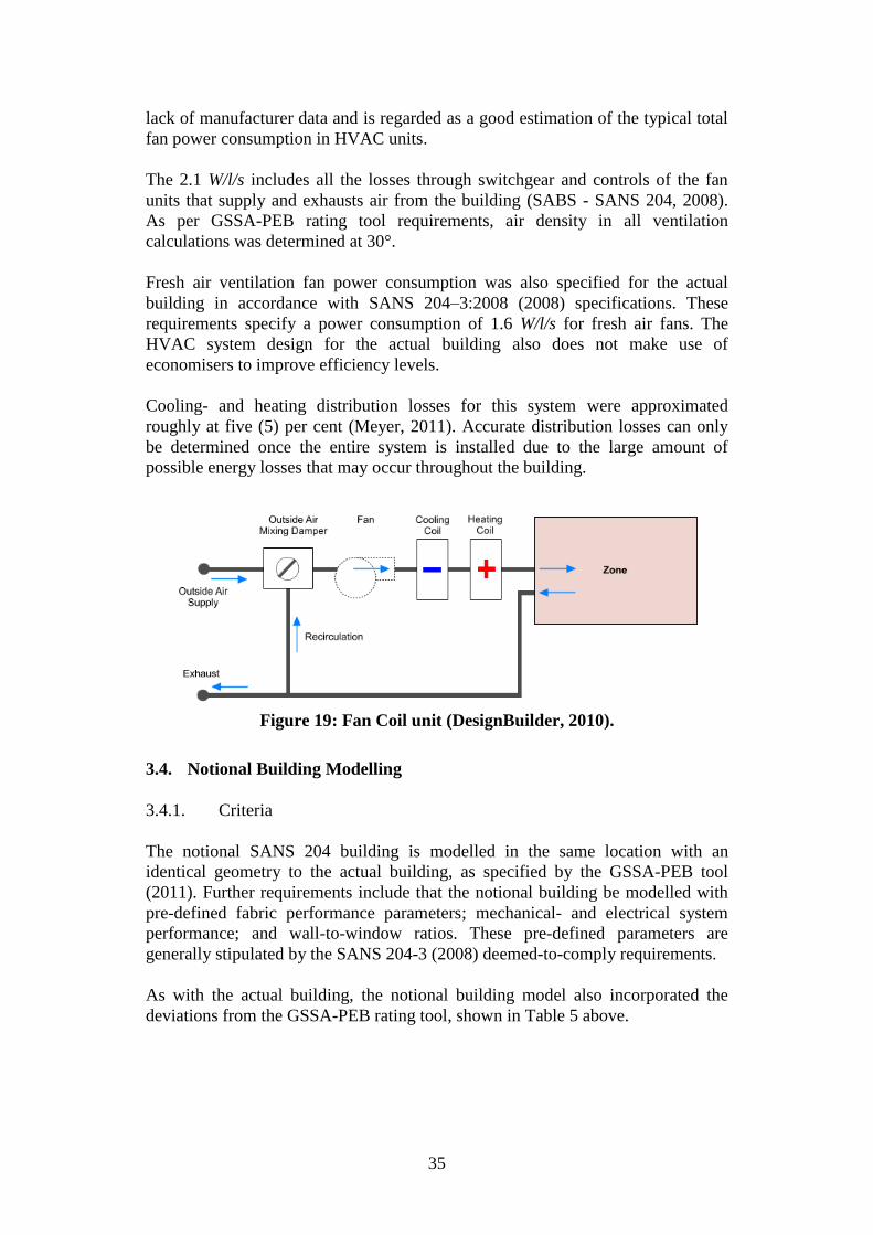
35
lack of manufacturer data and is regarded as a good estimation of the typical total
fan power consumption in HVAC units.
The 2.1 W/l/s includes all the losses through switchgear and controls of the fan
units that supply and exhausts air from the building (SABS - SANS 204, 2008).
As per GSSA-PEB rating tool requirements, air density in all ventilation
calculations was determined at 30°.
Fresh air ventilation fan power consumption was also specified for the actual
building in accordance with SANS 204–3:2008 (2008) specifications. These
requirements specify a power consumption of 1.6 W/l/s for fresh air fans. The
HVAC system design for the actual building also does not make use of
economisers to improve efficiency levels.
Cooling- and heating distribution losses for this system were approximated
roughly at five (5) per cent (Meyer, 2011). Accurate distribution losses can only
be determined once the entire system is installed due to the large amount of
possible energy losses that may occur throughout the building.
Figure 19: Fan Coil unit (DesignBuilder, 2010).
3.4. Notional Building Modelling
3.4.1. Criteria
The notional SANS 204 building is modelled in the same location with an
identical geometry to the actual building, as specified by the GSSA-PEB tool
(2011). Further requirements include that the notional building be modelled with
pre-defined fabric performance parameters; mechanical- and electrical system
performance; and wall-to-window ratios. These pre-defined parameters are
generally stipulated by the SANS 204-3 (2008) deemed-to-comply requirements.
As with the actual building, the notional building model also incorporated the
deviations from the GSSA-PEB rating tool, shown in Table 5 above.

36
An additional internal design deviation from the GSSA-PEB tool has however
been included, namely that the same fresh air ventilation rate of 8 l/s per person
used for the entire conditioned area of the actual building, is also used for the
notional building. All GSSA-PEB tool (2011) operational schedules (see Section
3.2.5) and climate-control parameters (refer to Section 3.3.1 above) were
furthermore implemented in the notional building model.
A further deviation from the GSSA-PEB rating tool is that the notional building
incorporates the glazing specifications established by SANS 204-3 (2008)
deemed-to-comply requirements. These requirements also form part of the
reference GSSA Office V1 Energy Calculator and Modelling Protocol Guide
(GBCSA, 2010).
3.4.2. Modelling Data
The data presented in this section is only applicable to the simulation model of the
notional building. Only the most important aspects regarding the simulation
model of the notional building are discussed in this section.
3.4.2.1. Construction
The notional building relies on fixed fabric-performance parameters, as specified
by SANS 204-3 (2008) for buildings built according to the minimum
requirements of energy-efficient buildings. The building envelope performance
parameters specified by the GSSA-PEB tool is unique for each climate zone in
South Africa. This building falls under climatic zone 4, namely ‘temperate
coastal’ (refer to Section 2.6 above).
In Table 9 the GSSA-PEB tool specification of the major energy-consumption
related structural components for the climate zone 4 is shown. No surface
emissivity or absorptivity values for the roof or walls are specified by SANS 204
(2008), and as a result the actual building data was used.
Table 9: Notional building construction elements (GBCSA, 2010).
Construction
element
Thermal resistance
(m2K/W)
External surface
Characteristic Value
Roof 3.71 Emissivity 0.90
Absorptivity 0.26
External walls 2.2 Emissivity 0.94
Absorptivity 0.50
All external
windows 0.127
2 SHGF 0.81
Note: 1) Defined as per climatic zone of Figure 7. 2) Based on a clear single glazing element with
an aluminium frame.

37
SANS 204 requires an energy-efficient building to conform to the façade-glazing
requirements formula for each orientation section of the building (SABS - SANS
204, 2008):
∑ [
]
(15)
Where
Fa is the façade area;
EI is the energy index value for the specific climatic zone provided by
SANS 204;
An is the area of each glazing element;
Sn is the SHGC of each glazing element;
CA,B,C is the energy constant provided by SANS 204;
SHn is the heating-shading multiplier provided by SANS 204;
SCn is the cooling-shading multiplier provided by SANS 204; and
Rn is the thermal resistance value of each glazing element (more
generally defined as a U-value, which is the reciprocal of the R-
value).
This formula can however be simplified to provide the percentage of glazing
required for the notional building in each of the four building façade orientations
(as measured from true North). The simplification is done by replacing some
variables with known values for minimum SANS 204 (2008) requirements.
Table 10: SANS 204 (2008) minimum glazing requirements.
Variable Value Reason
EI 0.22 Provided as a fixed constant.
Sn 0.77 Minimum required SHGC for climatic zone 41.
CA - 23° orientation -0.38
Provided as a fixed constant for each specific
building façade orientation2.
CA - 113° orientation -0.82
CA - 203° orientation -0.90
CA - 293° orientation -0.61
CB - 23° orientation 1.66
Provided as a fixed constant for each specific
building façade orientation2.
CB - 113° orientation 0.80
CB - 203° orientation 0.66
CB - 293° orientation 1.34
CC - 23° orientation -0.01 Provided as a fixed constant for each specific
building façade orientation2.
CC - 113° orientation 0.11
CC - 203° orientation 0.13

38
CC - 293° orientation 0.03
SHn 1.00 Based on minimum SANS 204 assumptions3.
SCn 1.00 Based on minimum SANS 204 assumptions3.
Rn 0.179 Minimum required R-value for climatic zone 41.
Notes: 1) Climatic zones are as defined in Figure 7 above. 2) The four building façade orientations
are measured from true North and constants are defined for each orientation section as defined in
Figure 3 of the SANS 204 – 3: 2008 energy-efficient building regulations (SABS - SANS 204,
2008). 3) To meet minimum SANS 204 requirements it has been assumed that all overhangs are
distanced more than 1.2 m apart from the top of each glazing element. SANS 204 specifies a value
of one (1) in climate zone 4 for both SHn and SCn under such conditions (SABS - SANS 204,
2008).
By substituting the variables listed in Table 10 into Equation 12, each of the
building façade orientation window-to-wall percentages can be calculated. These
window-to-wall percentages are provided in Table 11 and demonstrated in
Figure 20 below.
Table 11: Notional building window-to-wall percentage.
Building façade orientation Window-to-wall percentage
23° 23.67 %
113° 36.63 %
203° 40.50 %
293° 30.13 %
Figure 20: 113° Façade glazing representation of the actual building (left) and
the notional building (right).
Glazing element shading in the notional building is the same as with the actual
building. Neither SANS 204 nor the GSSA-PEB rating tool specifies shading for
notional buildings other than the actual fitted data.

39
3.4.2.2. Building Electrical Loads
Both the actual and notional buildings were simulated with the same equipment
loads (refer to Appendix E). All assumptions in the calculation of equipment loads
and thermal effects incorporated in the notional building simulation model were
the same as for the actual building (refer to Section 3.3.2.2 above).
The GSSA-PEB rating tool’s internal lighting power densities, as specified by the
UK Department of Communities and local Government: National Calculation
Method (DCLG, 2008), was used for the notional building. This was achieved by
matching each building zone with the most relevant GSSA-PEB rating tool
category.
The general methodology of the GSSA is to encourage the use of energy-efficient
lighting designs whilst achieving the appropriate light intensity levels. Typical
GSSA lighting intensity specifications are 400 lux at a working desk and 100 lux
in walkways (GBCSA, 2008). For an education building, therefore, the notional
building has a relatively low lighting power density of 9.76 W/m2.
The elevator energy usage has also been calculated according to Equation 12
above. The only difference in elevator energy usage between the notional and
actual building is that the GSSA-PEB tool specifies a 10kW elevator drive motor
for each elevator installed in the building. By substituting the 5.6 kW KONE drive
motor with a 10 kW GSSA-PEB specified motor; the annual elevator energy
consumption is calculated as 32.850 MW.
DHW energy use was furthermore calculated according to Equation 13 with the
same volume of water as the actual building DHW, but with five (5) per cent less
efficiency. This results in an annual DHW power consumption of 7.994 MWh.
3.4.2.3. HVAC
All HVAC system design parameters for the notional SANS 204 building were
based on SANS 204 (2008) specifications, as specified by the GSSA-PEB tool.
These parameters are shown Table 12 below.
Table 12: Notional building HVAC design parameters (GBCSA, 2010) (SABS
- SANS 204, 2008).
Design parameter Value
Cooling
Provided by air- cooled chiller with performance
characteristics based on Figure 22. Supply air
temperature is 12°C.
Heating Thermal electric reheat. Supply air temperature
is 30°C.

40
Chilled water pumps Pump power consumption is based on 349 W/l/s.
Air handling units Fan power is 2.1 W/l/s. This includes all losses
associated with supply and extraction fans.
Fresh air fans Fan power consumption is based on 1.6 W/l/s.
The air distribution system used for this building is based on a variable air volume
(VAV) supply system. Due to the ability to supply air according to the demand of
each zone, these systems are more efficient that constant volume systems.
Air supply and -demand in a VAV system are managed by controlling the central
fan speed to maintain static pressure in the air ducts and by adjusting the dampers
in the VAV control boxes located in each air-conditioned zone (Moult, 1999).
These VAV terminal units in the notional building simulation model were
configured to restrict air supply to a minimum of 30% of the designed air flow to
each zone.
Heating in the notional building is provided by terminal reheat coils in the zone
terminal unit, as prescribed by the GSSA-PEB rating tool. Further GSSA-PEB
requirements incorporated into the notional building HVAC design were to ensure
that no HVAC system heat recovery is done and no economisers are used for
energy demand reduction. Air distribution or leakage losses were furthermore not
accounted for in the ventilation system and HVAC system controls were set to
prevent both the heating and the cooling of air at the same time.
Figure 21: VAV air handling unit (adapted from DesignBuilder, 2010).
The notional building’s chiller performance characteristics are based on the
ASHRAE standard 90.1-2007 and rated at COP ≥ 2.80 and IPLV ≥ 3.05
(ASHRAE, 2007). These notional chiller operational performance characteristics
are depicted in Figure 22 below.
Zone 2, Zone 3 etc. below

41
A full performance analysis and comparison of the actual and notional building
chillers is presented in Section 3.5 below.
Figure 22: Notional building chiller performance curve (GBCSA, 2011).
3.5. Simulation Data
3.5.1. Simulation Methodology
DesignBuilder was used to determine the fabric and ventilation performance data;
internal gains; and occupants’ comfort assessments on both buildings. Raw
EnergyPlus data was however used to determine the annual HVAC energy
consumption information. This approach was chosen due to the small HVAC
result interpretational differences between EnergyPlus and DesignBuilder.
The convection algorithms used in both buildings were the EnergyPlus Adaptive
Convection Algorithm (2010) for inside convection and the DOE-2 Convection
Algorithm (EnergyPlus, 2010) for outside convection. Internal environment
control was achieved by controlling the air and not the operative temperature. All
surrounding buildings were furthermore included in shading calculations and the
effects of shading and reflections were included in the measurement of ground-
reflected solar.
The notional building’s energy flow data was calculated by editing the raw
EnergyPlus input file produced by DesignBuilder to reflect the operating
conditions of the SANS 204 chiller. After running the EnergyPlus simulation, the
data was imported back into DesignBuilder for building fabric- and comfort
2.25
2.75
3.25
3.75
4.25
4.75
1 2 3 4 5 6 7 8 9 10
EER
Normalised Load
SANS 204: 20 deg C
SANS 204: 35 deg C

42
assessments. Notional building HVAC data was however interpreted directly from
the EnergyPlus output file.
Chiller interpretation of the actual building was done in DesignBuilder; the
editing of raw EnergyPlus data was therefore not necessary. Only the HVAC
pump energy consumption was calculated in the actual building EnergyPlus file.
The mechanical ventilation fan’s airflow rate in the actual building was
determined by substituting the fan-coil ventilation system with a VAV system and
re-simulating the model with EnergyPlus. This was done because it is assumed
that the air supply of each fan-coil unit will be varied according to the demand in
each zone.
Heating energy in the actual building was furthermore calculated by defining a
simple HVAC system that has all the characteristics of the actual system, but with
the ability to accommodate different COP heating values for each zone (refer to
Appendix F, Table 26).
Table 13: Simulation results data origination.
Category Data origination
Actual building Notional building
Building fabric and
ventilation performance DesignBuilder model DesignBuilder model
PMV comfort DesignBuilder model DesignBuilder model
Heating
DesignBuilder model
with simple HVAC
system definition
DesignBuilder model
Cooling Raw EnergyPlus data Raw EnergyPlus data
Pumps Raw EnergyPlus data Raw EnergyPlus data
Fans
Raw EnergyPlus data
from VAV HVAC
DesignBuilder model
Raw EnergyPlus data
Extract & Misc. fans GSSA-PEB calculation GSSA-PEB calculation
Lighting DesignBuilder model DesignBuilder model
Equipment DesignBuilder model DesignBuilder model
Vertical transportation GSSA-PEB calculation GSSA-PEB calculation
DHW GSSA-PEB calculation GSSA-PEB calculation
The first design stage data of the actual building used in this study included no on-
site renewable energy sources. No annual energy deductions were therefore made
to the actual building in the comparative analysis between the actual and notional
building (refer to section 2.5.3).
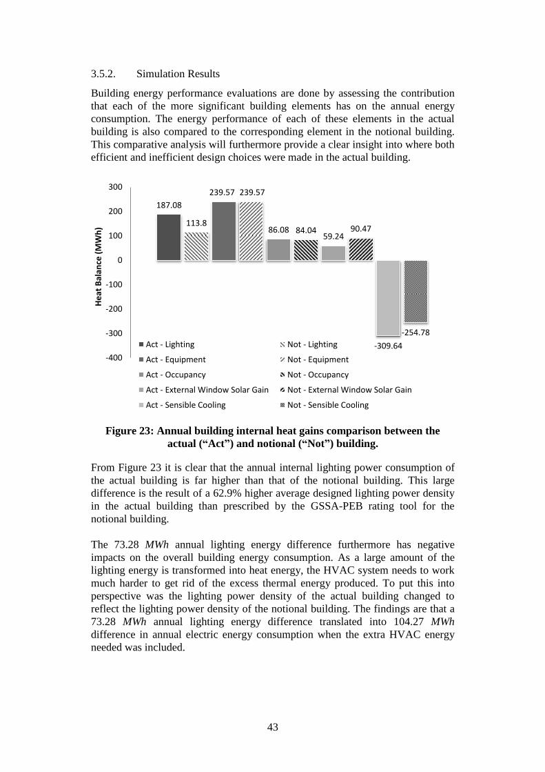
43
3.5.2. Simulation Results
Building energy performance evaluations are done by assessing the contribution
that each of the more significant building elements has on the annual energy
consumption. The energy performance of each of these elements in the actual
building is also compared to the corresponding element in the notional building.
This comparative analysis will furthermore provide a clear insight into where both
efficient and inefficient design choices were made in the actual building.
Figure 23: Annual building internal heat gains comparison between the
actual (“Act”) and notional (“Not”) building.
From Figure 23 it is clear that the annual internal lighting power consumption of
the actual building is far higher than that of the notional building. This large
difference is the result of a 62.9% higher average designed lighting power density
in the actual building than prescribed by the GSSA-PEB rating tool for the
notional building.
The 73.28 MWh annual lighting energy difference furthermore has negative
impacts on the overall building energy consumption. As a large amount of the
lighting energy is transformed into heat energy, the HVAC system needs to work
much harder to get rid of the excess thermal energy produced. To put this into
perspective was the lighting power density of the actual building changed to
reflect the lighting power density of the notional building. The findings are that a
73.28 MWh annual lighting energy difference translated into 104.27 MWh
difference in annual electric energy consumption when the extra HVAC energy
needed was included.
187.08
113.8
239.57 239.57
86.08 84.04 59.24
90.47
-309.64
-254.78
-400
-300
-200
-100
0
100
200
300
He
at B
alan
ce (
MW
h)
Act - Lighting Not - Lighting
Act - Equipment Not - Equipment
Act - Occupancy Not - Occupancy
Act - External Window Solar Gain Not - External Window Solar Gain
Act - Sensible Cooling Not - Sensible Cooling

44
A further observation made from Figure 23 is that the notional building has
considerably more solar thermal energy gain than the actual building. The reason
for this can be found by comparing the glazing SHGF (Table 6 and Table 9) and
area (Table 4 and Table 11) in each building. This data indicates that the
substantial difference between solar heat gain of the notional and actual building
is a result of a larger glazing area, higher SHGF and higher thermal conduction
capacity of the glazing elements in the notional building. Figure 24 however
shows that these properties of the notional building glazing elements also result in
more heat loss in the winter.
Figure 24: 3.8° Celsius building fabric performance comparison between the
actual (“Act”) and notional (“Not”) building.
From Figure 24 one also notices the large difference in heat loss through the
external walls. This can be attributed firstly to the 1.188 m2K/W difference in
external wall thermal insulation between the notional and actual building; and
secondly to the difference in external wall area as a result of the window-to-wall
ratios.
Another fairly significant difference between the fabric performance data of the
actual and the notional building is the roof insulation. The actual building roof is
23.7% better-insulated than the notional building roof, and thus permits less heat
flow to occur in the winter.
Figure 24 furthermore shows the heat energy storage capabilities of the thermal
mass in the building floors (excluding the ground floor) and the effect of ground
temperatures on the ground floor. The reason why the ground temperatures have a
large impact on the ground floor is because the actual building ground floor
-26.67
-39
-19.46
-8.11
0.47 0.31
-1.35 -1.35 -3.31 -4.35
-71.19 -71.17 -80
-70
-60
-50
-40
-30
-20
-10
0
10
He
at B
alan
ce (
kW)
Act - Glazing Not - Glazing
Act - Walls Not - Walls
Act - Floors Not - Floors
Act - Ground Floor Not - Ground Floor
Act - Roof Not - Roof
Act - External Ventilation Not - External Ventilation

45
design incorporates no insulation layers. Heat loss through the ground floor in this
building, however, is beneficial due to the large internal heat loads.
Figure 25: Actual building Open Plan Office 2 summer design week PMV.
The typical occupant comfort to be expected in Open Plan Office 2 on the fourth
floor of the actual building (refer to Appendix B) during a typical hot summer
week in January is shown in Figure 25 above. The comfort level pursued in this
zone is a PMV index of zero (0) during occupancy hours to ensure an optimally
comfortable environment for the occupants (refer to Section 2.2).
Because the HVAC system has the largest impact on occupant comfort in a
mechanically air-conditioned building, the operational characteristics of the
HVAC system are typically reflected in the PMV index. This is also evident in the
PMV data presented in Figure 25 where the GSSA-PEB rating tool occupancy
hours specified for this zone range between 7am and 8pm on weekdays.
The cooling overshoot shown in data point 1 of Figure 25 can be attributed to a
relatively small zone served by a fan-coil unit that has the ability to cool the zone
at a faster rate as opposed to a big central unit with more thermal inertia. This
slow response of the high thermal inertia in the notional building’s central VAV
HVAC system is seen in the PMV data of Figure 26 for the same zone and
timeframe as the actual building data of Figure 25 above.
Data point 2 in Figure 25 shows a rapid internal environment temperature change
when the HVAC system is turned off. This steep decline in thermal comfort can
be attributed to the combined effect of thermal energy stored in the external
building envelope and the outdoor temperature.
1
2

46
Further detailed simulation analysis results for Open Plan Office 2 are given in
Appendix H. This was done to evaluate the annual energy performance of the
building fabric and systems on a zone level.
Figure 26: Notional building Open Plan Office 2 summer design week PMV.
As mentioned in Section 3.2.5 above, all building occupancy and operational
loads are controlled by fixed schedules. The effects that these schedules have on
heat gain in both buildings, and the resulting cooling energy needed to create a
comfortable environment, are seen in Figure 27 and Figure 28 below.
These figures also show that collective heat gain of the building’s operational
loads far exceeds the heating energy required throughout the largest part of the
day. There is however a short period in the morning when HVAC heating energy
is needed. This period spans between the time when the HVAC system is
switched on and the time when the combined thermal effect of the building
operational loads and solar energy exceeds the building heating requirement.
These figures furthermore illustrate why a central VAV unit is more energy-
efficient than numerous small fan-coil units. This energy efficiency advantage is
due to an intelligent whole-building supply and demand control system; less fan
and piping losses; and the dampening effect caused by a large amount of thermal
inertia in the VAV ventilation system.
Neither the notional building- nor the actual building HVAC system incorporates
economisers. This implies that both the actual and notional building will have to
provide cooling energy through the HVAC system to balance the heating effects
of operational loads. The reason for this is that constant partial recirculation

47
occurs in the ventilation system of both buildings and only a fraction of the air is
replaced with fresh air (depending on zone occupancy). The resulting relatively
warm combination of fresh and recirculated air therefore requires HVAC cooling
energy through most of the winter.
Figure 27: Actual building typical winter day hourly internal gains.
Figure 28: Notional building typical winter day hourly internal gains.

48
The contribution of each energy category to the annual energy consumption of
both buildings is depicted in Figure 29 below. It should however be noted that this
building energy performance analysis is based on typical operational conditions
derived from GSSA-PEB tool requirements and will therefore only be an
approximation of the annual energy consumption per category.
Figure 29: Energy consumption category comparison between the actual
building (top) and the notional building (bottom).
It should furthermore be noted that both models incorporated deviations from the
GSSA-PEB rating tool to do a more realistic building energy performance
comparison. Due to the large difference in lighting energy requirements and the
relatively small possible impact of the GSSA-PEB rating tool deviations,
however, this building does not fulfil the conditional requirements of the GSSA-
PEB rating tool (refer to Section 2.5.1), given that no renewable energy is
generated on-site.
Heating
Cooling
Pumps
Fans
Extract & Misc Fans
Lighting
External Lighting
Vertical Transport
DHW
Equipment
Heating
Cooling
Pumps
Fans
Extract & Misc Fans
Lighting
External Lighting
Vertical Transport
DHW
Equipment

49
Table 14 below shows the results of a comparative annual building energy
performance assessment done between the actual and notional building. The
actual building energy performance percentage of each category listed in Table 14
is calculated as a percentage the difference in energy consumption between the
actual and notional building in each category, has on the total annual energy
consumption of the notional building.
Table 14: Actual building’s energy performance evaluation.
Energy
category
Actual building
annual electrical
energy use (kWh)
Notional building
annual electrical
energy use (kWh)
Actual building
energy
performance
Heating 4503 2124 -0.37%
Cooling 224786 219324 -0.84%
Pumps 21212 9120 -1.86%
Fans 44752 16360 -4.36%
Extract & Misc.
Fans 3706 3794
0.01%
Lighting 187078 113800 -11.25%
External
Lighting 5077 5077
0.00%
Vertical
Transportation 19053 32850
2.12%
DHW 7573 7994 0.06%
Equipment 241062 241062 0.00%
Total 758802 651505 -16.47%
The carbon footprint of both buildings is calculated by using the conversion factor
of 1.2 kg CO2/kWh provided by ESKOM (2007). This results in an annual carbon
footprint for the actual building of 911 ton CO2 and 782 ton CO2 for the notional
building.
A further comparative analysis was done to determine the energy performance of
the building area that the new Centre for Renewable and Sustainable Energy
Studies (CRSES) will occupy. The zones included in this assessment are shown in
Table 27, Appendix G. It should however be noted that this assessment only gives
an indication of the energy performance of the zones which CRSES is comprised
of and does not take into account the effect of the other adjacent building zones.
Simulation results of this analysis are shown below in Table 15.
The actual building CRSES energy performance difference depicted in Table 15
gives an indication which energy category has the largest influence on the overall
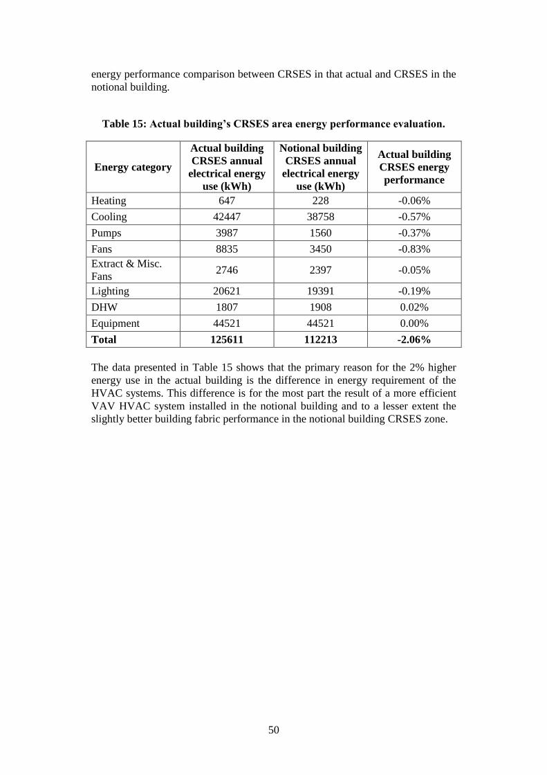
50
energy performance comparison between CRSES in that actual and CRSES in the
notional building.
Table 15: Actual building’s CRSES area energy performance evaluation.
Energy category
Actual building
CRSES annual
electrical energy
use (kWh)
Notional building
CRSES annual
electrical energy
use (kWh)
Actual building
CRSES energy
performance
Heating 647 228 -0.06%
Cooling 42447 38758 -0.57%
Pumps 3987 1560 -0.37%
Fans 8835 3450 -0.83%
Extract & Misc.
Fans 2746 2397 -0.05%
Lighting 20621 19391 -0.19%
DHW 1807 1908 0.02%
Equipment 44521 44521 0.00%
Total 125611 112213 -2.06%
The data presented in Table 15 shows that the primary reason for the 2% higher
energy use in the actual building is the difference in energy requirement of the
HVAC systems. This difference is for the most part the result of a more efficient
VAV HVAC system installed in the notional building and to a lesser extent the
slightly better building fabric performance in the notional building CRSES zone.

51
4. PARAMETRIC ANALYSIS
As a result of the large energy performance differences between the actual and
notional building, a parametric analysis was done to investigate the possibility of
improving the actual building energy performance. The objective of this analysis
was to determine the effect that a change in building fabric and building systems
operational efficiency may have on the annual energy consumption of the
building. Each of these possible improvements was assessed in three main
categories, which are building fabric, HVAC and lighting.
4.1. Building Fabric
The building fabric properties identified in Section 3.5 as elements in the actual
building that have the most room for improvement are as follows:
External wall insulation and thermal mass properties;
Glazing type and building wall-to-window ratio; and
Roof insulation properties.
4.1.1. External walls
External wall insulation and thermal mass properties were changed by filling the
50mm air cavity between the two 110mm brick layers of the actual building
external walls with materials that has different thermal resistance and mass
properties. Each of the filling materials chosen for this parametric wall test was
materials that can be used to fill the air cavity at an advanced stage of
construction.
Table 16 below shows the results of an annual energy performance comparison on
the actual building where the external wall properties was changed for each
parametric simulation. The energy performance difference depicted in this table
shows an annual energy performance improvement as a negative difference and
vice versa.
Table 16: Annual building energy performance in terms of external wall’s
cavity-filling material.
Cavity filling
material
Total wall R-value
(m2K/W)
Annual energy performance
difference (kWh)
Dense concrete 0.87 -10190
Aerated concrete 1.00 -2987
Air 1.01 0
EPS polystyrene 1.92 2700
Polystyrene beads 2.22 3304

52
From Table 16 it can be seen that walls with a better insulation increases annual
energy consumption in this building. This anti-insulation behaviour can
predominantly be attributed to the large internal heat load generated by building
operational loads; a relatively warm climate throughout the year; and the cooling
set-point temperature of the HVAC system. Masoso & Grobler (2008) describe
this behaviour as a “point of thermal inflection” where a higher thermal resistance
of the external building fabric insulation increases the annual energy consumption
of the building.
The reason why the aerated and dense concrete cavity filling reduces annual
energy consumption may be contributed to the combination of an increase in
thermal mass and, to a lesser extent, the reduction of thermal resistance. An
increase in thermal inertia of building walls reduces the internal air temperature
variation of the building, and thus lowers the mechanical air-conditioning load
(Balaras, 1995). Effective utilisation of this natural cooling and heating source is
however greatly influenced by the thermodynamic properties of the materials that
the thermal mass are composed of; the level of thermal mass access; and the heat
transfer efficiency between the zone and the thermal mass (Shaw, et al., 1994).
4.1.2. Glazing
The actual building’s glazing properties were evaluated by determining the effect
of a variation in external window-to-wall ratio and glazing type. Figure 30 below
shows the annual energy consumption increase as a function of window-to-wall
ratio.
Figure 30: Building façade glazing effect on annual energy consumption.
-2000
0
2000
4000
6000
8000
10000
20% 30% 40% 50% 60% 70% 80%
An
nu
al b
uild
ing
en
erg
y co
nsu
mp
tio
n
incr
eas
e (
kWh
)
Façade glazing percentage
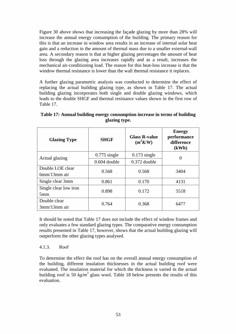
53
Figure 30 above shows that increasing the façade glazing by more than 28% will
increase the annual energy consumption of the building. The primary reason for
this is that an increase in window area results in an increase of internal solar heat
gain and a reduction in the amount of thermal mass due to a smaller external-wall
area. A secondary reason is that at higher glazing percentages the amount of heat
loss through the glazing area increases rapidly and as a result, increases the
mechanical air-conditioning load. The reason for this heat-loss increase is that the
window thermal resistance is lower than the wall thermal resistance it replaces.
A further glazing parametric analysis was conducted to determine the effect of
replacing the actual building glazing type, as shown in Table 17. The actual
building glazing incorporates both single and double glazing windows, which
leads to the double SHGF and thermal resistance values shown in the first row of
Table 17.
Table 17: Annual building energy consumption increase in terms of building
glazing type.
Glazing Type SHGF Glass R-value
(m2K/W)
Energy
performance
difference
(kWh)
Actual glazing 0.775 single 0.173 single
0 0.604 double 0.372 double
Double LOE clear
6mm/13mm air 0.568 0.568 3404
Single clear 3mm 0.861 0.170 4131
Single clear low iron
5mm 0.898 0.172 5518
Double clear
3mm/13mm air 0.764 0.368 6477
It should be noted that Table 17 does not include the effect of window frames and
only evaluates a few standard glazing types. The comparative energy consumption
results presented in Table 17, however, shows that the actual building glazing will
outperform the other glazing types analysed.
4.1.3. Roof
To determine the effect the roof has on the overall annual energy consumption of
the building, different insulation thicknesses in the actual building roof were
evaluated. The insulation material for which the thickness is varied in the actual
building roof is 50 kg/m3 glass wool. Table 18 below presents the results of this
evaluation.

54
Table 18: Annual building energy performance in terms of roof insulation
properties.
50 kg/m3 glass wool roof
insulation thickness
Roof R-value
(m2K/W)
Energy performance
difference (kWh)
26mm 2.58 224
63mm 3.58 95
100mm 4.58 0
130mm 5.58 -26
167mm 6.58 -79
From Table 18 it is evident that a variation in roof insulation properties has a
minimal effect on the total annual energy consumption of the building. The local
energy consumption and occupant comfort impact on the fourth-floor and
mezzanine will however be higher. An R-value of lower than 2.5 was thus not
considered for the evaluation to ensure that the occupant comfort index
experienced on the mezzanine is taken into account.
4.2. Lighting System Efficiency
As mentioned in Section 3.5, a simulation model was created to determine the
annual energy consumption of the actual building when the actual building’s
lighting system is replaced with the lighting system of the notional building. The
reason for this analysis is that the notional building lighting system has a
significantly smaller installed lighting capacity of 33 350 kW compared to the
55 062 kW of the actual building (refer to Appendix C).
The simulation results revealed that the 21 712 kW excess lighting power installed
in the actual building translates into an annual lighting energy consumption
difference of 73 278 MWh. This excess lighting power furthermore results in a
HVAC load increase of 30 992 kWh.
The total annual energy consumption difference between the actual and notional
building is 108 188 kWh. The difference however between the annual energy
consumption of the actual building and the actual building with a notional
building lighting power density is 104 270 kWh. Therefore, by only reducing the
lighting energy density of the actual building to the lighting energy density of the
notional building, the resulting energy performance difference between the two
buildings is reduced to only 0.6%.
From a cost perspective would a 62.9% reduction in the lighting power density of
the actual building not necessarily imply a lower initial capital expenditure. The
cost implications however of reducing the annual energy consumption of the
actual building by reducing the lighting levels to the levels specified for the

55
notional building over the projected lifetime of the building is significant. To put
this into perspective was a 5 year cost analysis done where zero (0) excess initial
capital expenditure is assumed and a fixed annual operational and maintenance
cost of R 16 500 is deducted (2% of total lighting cost). The results of this
analysis are shown in Table 19 below.
Table 19: Cost summary of lighting system energy reduction.
Year
Present value of
annual
income/expense(1)
Net present
value
Annual
electricity price
increase(2)
Electricity
price per
kWh (3)
2011 R 0.00 R 0.00 - R 1.14
2012 R 94 785.00 R 94 785.00 25.90% R 1.44
2013 R 114 158.57 R 208 943.57 10.00% R 1.58
2014 R 117 582.44 R 326 526.02 10.00% R 1.74
2015 R 120 972.70 R 447 498.71 10.00% R 1.91
2016 R 124 335.89 R 571 834.61 10.00% R 2.10
Note: 1) Annual income calculated by determining the energy cost equivalent of 104,270 MWh.
2) The first year price increase was determined from ESKOM (2011) data. Price increases for year
two and further was estimated at 10% annually. 3) Data obtained from Krige (2011).
The annual cost savings presented in Table 19 was determined by calculating the
present and net present value of an annual energy saving of 104,270 MWh when
the effect of rising electricity costs and inflation is included. The net present
value (NPV) of money used in Table 19 abides by the following formula:
∑
(16)
In equation (16), R is the net cash flow of each year, N is the time in years and
DCR is the opportunity cost of capital or discount rate. For the NPV values
presented in Table 19, was a annual DCR of 8% used to reflect the estimated
inflation for the next five years and the net cash flow used as the annual energy
cost equivalent of 104 270 MWh. The present values shown in Table 19 above
gives an indication of what the value of the energy cost saving each year is when
it is discounted to the year 2011. These values were calculated by using N = 1 in
Equation 16 for each specific year.
4.3. HVAC System Efficiency
A further parametric simulation was done to determine the difference in annual
energy consumption that the actual building will have when it’s fan-coil HVAC
system is replaced with a VAV system. The addition of a temperature-controlled
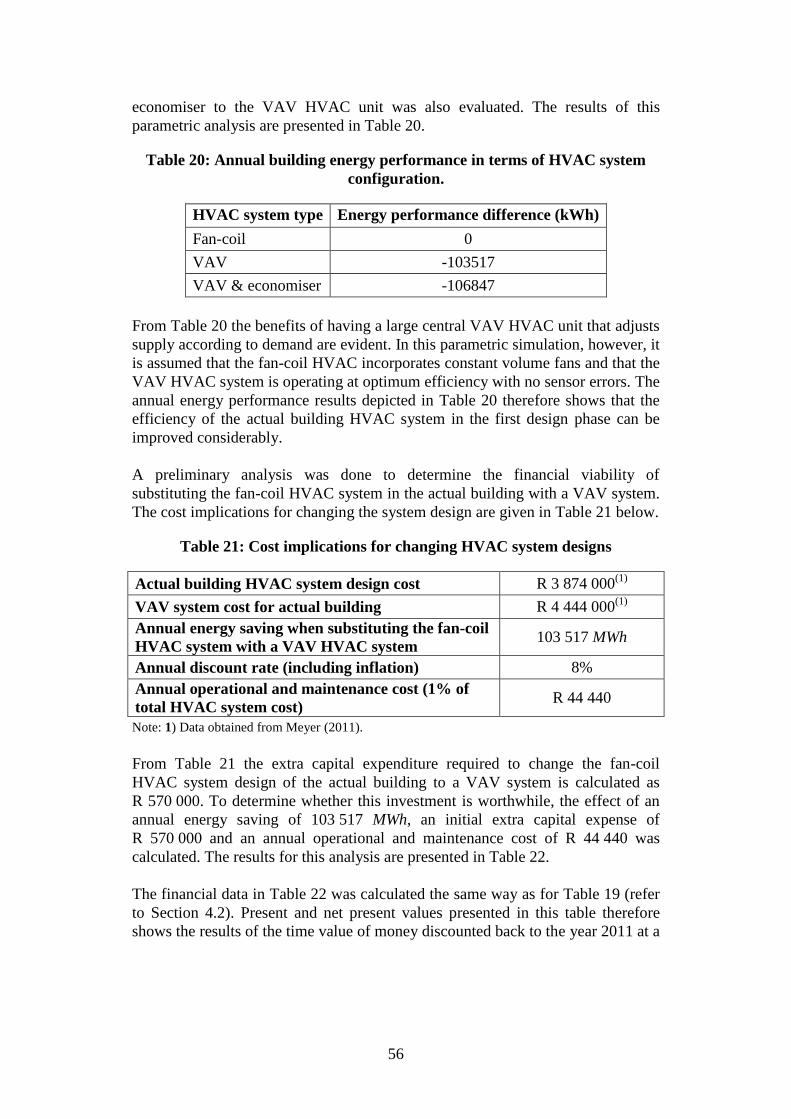
56
economiser to the VAV HVAC unit was also evaluated. The results of this
parametric analysis are presented in Table 20.
Table 20: Annual building energy performance in terms of HVAC system
configuration.
HVAC system type Energy performance difference (kWh)
Fan-coil 0
VAV -103517
VAV & economiser -106847
From Table 20 the benefits of having a large central VAV HVAC unit that adjusts
supply according to demand are evident. In this parametric simulation, however, it
is assumed that the fan-coil HVAC incorporates constant volume fans and that the
VAV HVAC system is operating at optimum efficiency with no sensor errors. The
annual energy performance results depicted in Table 20 therefore shows that the
efficiency of the actual building HVAC system in the first design phase can be
improved considerably.
A preliminary analysis was done to determine the financial viability of
substituting the fan-coil HVAC system in the actual building with a VAV system.
The cost implications for changing the system design are given in Table 21 below.
Table 21: Cost implications for changing HVAC system designs
Actual building HVAC system design cost R 3 874 000(1)
VAV system cost for actual building R 4 444 000(1)
Annual energy saving when substituting the fan-coil
HVAC system with a VAV HVAC system 103 517 MWh
Annual discount rate (including inflation) 8%
Annual operational and maintenance cost (1% of
total HVAC system cost) R 44 440
Note: 1) Data obtained from Meyer (2011).
From Table 21 the extra capital expenditure required to change the fan-coil
HVAC system design of the actual building to a VAV system is calculated as
R 570 000. To determine whether this investment is worthwhile, the effect of an
annual energy saving of 103 517 MWh, an initial extra capital expense of
R 570 000 and an annual operational and maintenance cost of R 44 440 was
calculated. The results for this analysis are presented in Table 22.
The financial data in Table 22 was calculated the same way as for Table 19 (refer
to Section 4.2). Present and net present values presented in this table therefore
shows the results of the time value of money discounted back to the year 2011 at a
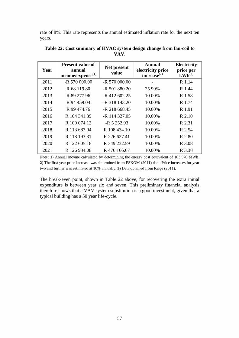
57
rate of 8%. This rate represents the annual estimated inflation rate for the next ten
years.
Table 22: Cost summary of HVAC system design change from fan-coil to
VAV.
Year
Present value of
annual
income/expense(1)
Net present
value
Annual
electricity price
increase(2)
Electricity
price per
kWh(3)
2011 -R 570 000.00 -R 570 000.00 - R 1.14
2012 R 68 119.80 -R 501 880.20 25.90% R 1.44
2013 R 89 277.96 -R 412 602.25 10.00% R 1.58
2014 R 94 459.04 -R 318 143.20 10.00% R 1.74
2015 R 99 474.76 -R 218 668.45 10.00% R 1.91
2016 R 104 341.39 -R 114 327.05 10.00% R 2.10
2017 R 109 074.12 -R 5 252.93 10.00% R 2.31
2018 R 113 687.04 R 108 434.10 10.00% R 2.54
2019 R 118 193.31 R 226 627.41 10.00% R 2.80
2020 R 122 605.18 R 349 232.59 10.00% R 3.08
2021 R 126 934.08 R 476 166.67 10.00% R 3.38
Note: 1) Annual income calculated by determining the energy cost equivalent of 103,570 MWh.
2) The first year price increase was determined from ESKOM (2011) data. Price increases for year
two and further was estimated at 10% annually. 3) Data obtained from Krige (2011).
The break-even point, shown in Table 22 above, for recovering the extra initial
expenditure is between year six and seven. This preliminary financial analysis
therefore shows that a VAV system substitution is a good investment, given that a
typical building has a 50 year life-cycle.
58
5. CONCLUSIONS
The aim of this study was to determine and evaluate the energy performance of
the new academic building to be built at Stellenbosch University. These
evaluations were done by comparing the actual building’s annual energy
consumption with a notional building that is built according to minimum SANS
204 energy-efficient building requirements, as interpreted by the GSSA-PEB
green building rating tool.
Building energy consumption improvement options identified in this study did not
take into account the outcome of a comprehensive cost-benefit analysis over the
lifetime of the building. The emphasis was rather placed on the reduction of
energy consumption of the inefficient components in the building to a level where
the GSSA energy criteria conditional requirements would be satisfied.
The energy modelling comparison revealed that the actual building is consuming
16.5% more energy than the notional building on an annual basis, and therefore
does not qualify for a GSSA accreditation. However, as noted in Section 3.5, is
this annual energy performance difference subject to variation as changes to the
initial design may be implemented throughout the building construction phase.
The annual energy consumption results of both buildings are furthermore subject
to the operational profiles of general education buildings and typical loads
specified by the GSSA-PEB tool due to the unavailability of actual operational
data in the building design phase.
One of the primary reasons identified for the poor energy performance of the
actual building in comparison with the notional building, is the designed lighting
density. This internal lighting density proved to be 63% higher than the GSSA-
PEB rating tool’s recommended lighting density. The overall impact on the annual
energy consumption proved to be even more due to the larger amount of cooling
energy necessary to offset the excess heat energy produced by the luminaries.
The cause of the high lighting power density in the actual building may partially
be attributed to the fact that all the lighting circuits in the building are manually
triggered and in some zones multiple lighting circuits are installed, for example
the lecture halls, to cater for different lighting requirements. Both these lighting
design properties have negative impacts on the annual energy consumption of the
building. The reason for this is that even though all the lights in the room are not
switched on every time a person walks into the room, the GSSA argues that the
person has the ability to switch on all the lights if no intelligent lighting control is
installed (GBCSA, 2008). All the lights in a zone that has no intelligent lighting
control are therefore modelled as either fully on or fully off, depending on the
lighting schedule of the room.

59
To reduce the internal lighting density of the actual building, however, it is not
just as simple as reducing the amount of luminaries. A good energy-efficient
lighting design should provide the optimum balance between:
Initial cost;
Maintenance cost;
Lighting power density;
Minimum lighting level building regulations; and
Lighting level uniformity and aesthetic appearance.
A brief financial analysis however revealed that a reduction in the lighting energy
density of the actual building to the levels specified for the notional building
would result in a considerable saving over the lifetime of the building.
The HVAC energy consumption in the actual building was also identified as one
of the components that can significantly influence the annual energy consumption
of the building. This is mostly because the ventilation system incorporated in the
actual building is significantly less efficient than a variable air volume system.
The parametric results presented in section 4.3 indicate that replacing the designed
fan-coil system with a VAV system can reduce the annual energy consumption
with 13% and result in a worthwhile investment over the building lifetime.
Comparative results of the building fabric performance furthermore revealed that
the actual building performs slightly better than the notional building. The actual
building’s fabric parametric analysis also showed that the cavity in the building
walls can be filled with concrete (or any substance with a low R-value and high
thermal mass) to improve the total annual energy consumption of the building.
This also emphasised the positive energy offset effect that a good thermal mass
design has on the building and the anti-insulation behaviour of the building fabric.
To ensure that a GSSA accreditation for the academic building is possible, the
primary focus should however be on reducing the lighting power density;
improving the efficiency of the HVAC system of the actual building; and
incorporating on-site renewable energy generation sources. An annual energy
performance improvement over the notional building for the actual building can
be accomplished by only reducing the lighting density of the building to the
recommended GSSA-PEB levels and marginally improving the energy efficiency
of the HVAC system.
The option of incorporating an on-site renewable as a possible energy offset for
the actual building was investigated in Appendix I. PV technology was chosen for
this investigation because a PV array is considered to be the only viable large on-
site renewable energy generation option for the new academic building. This
investigation showed that a solar system that is designed within the limits of what
CRSES can afford, can deliver an estimated 24 323 kWh of clean renewable
energy annually.

60
6. RECOMMENDATIONS AND FUTURE WORK
At the stage when this study was completed, a number of assumptions necessarily
had to be made as certain design choices were still to be finalised. It is therefore
recommended that the actual building simulation model be changed to reflect the
final design data and re-simulated to determine if small design changes made
through the design phase have enabled the building to be more energy efficient.
The comparative analysis between the notional and actual building also included a
few GSSA-PEB tool deviations to more closely reflect the expected operational
conditions of the building in this study. Even though the results presented in this
study closely reflect the energy performance difference between the actual and
notional building, the simulation model should be changed to fully conform to
GSSA-PEB requirements for a full GSSA accreditation assessment.
It is furthermore recommended that the design of the lighting- and HVAC system
be re-assessed with the primary aim of reducing the annual energy consumption.
The energy optimisation options identified in this study should also be evaluated
in terms of a full building, life-cycle cost-benefit scenario with the emphasis on
obtaining a green building energy efficiency rating.
An investigation should also be launched to determine the optimum efficient
operational profiles and procedures for building HVAC and electrical systems.
Such energy efficiency measures would typically result in a significant reduction
in annual energy consumption and life-cycle carbon emissions of the building.
It is lastly recommended that PV array on the roof of the new building (refer to
Appendix I) be considered as a natural renewable energy source for on-site
renewable energy generation to off-set the carbon footprint of the building.

61
REFERENCES
Al-Sanea, S. A., Zedan, M. & Al-Hussain, S., 2012. Effect of thermal mass on
performance of insulated building walls and the concept of energy savings
potential. Applied Energy, pp. 430-442.
Álvarez, C., Alcazar, M., Escrivá, G. & Gabaldón, A., 2009. Technical and
economical tools to assess customer demand response in the commercial
sector. Issue 50, pp. 2605-2612.
Arendse, G., 2011. Stellenbosch new engineering building electrical system
design. Stellenbosch: De Villiers & Moore Consulting Engineers.
Ashpole, M., 2009. Improving energy efficiency in buildings: SANS 204
published. Civil Engineering, March, 17(2), pp. 58-59.
ASHRAE, 2000. Advanced energy design guide for small office buildings,
Atlanta, USA: s.n.
ASHRAE, 2004. Standard 55: Thermal environment conditions for human
occupancy. s.l.:s.n.
ASHRAE, 2007. ASHRAE standard 90.1: Energy standard for buildings except
low-rise residential buildings, s.l.: s.n.
ATI, 2011. Alububble 1983: Technical datasheet. [Online].
Auliciems, A. & Szokolay, S. V., 2007. Thermal Comfort. Brisbane: Department
of Architecture, The University of Queensland.
Balaras, C., 1995. The role of thermal mass on the cooling load of buildings. An
overview of computational methods. Energy and Buildings, Volume 24, pp.
1-10.
Begemann, S., Van den Beld, G. & Tenner, A., 1996. Daylight, artificial light and
people in an office environment, overview of visual and biological
responses. International Journal of Industrial Ergonomics, Volume 20, pp.
231-239.
Cengel, Y. A., 2006. Heat and mass transfer: A practical approach. 3 ed. Reno,
Nevada: Mc Graw Hill.
Chapman, A. J., 1984. Heat Transfer. New York: Macmillan Publishing.
Cheng-wen, Y. & Jian, Y., 2010. Application of ANN for the prediction of
building energy consumption at different climate zones with HDD and

62
CDD. Second International Conference on Future Computer and
Communication, Volume 3, pp. 286-289.
Corgnati, S. P., Fabrizio, E. & Filippi, M., 2008. The impact of indoor thermal
conditions, system controls and building types on the building energy
demand. Energy and Buildings, 40(4), pp. 627-636.
Cornell University, 2011. College of Architecture. [Online]
Available at: http://aap.cornell.edu/milstein/design/sustainability.cfm
Corobrick, 2009. Towards a balanced and better understanding of the thermal
performance and sustainability of walling envelopes as marketed in South
Africa, Johannesburg: s.n.
Crawley, D. B., Lawrie, L. K., Pedersen, C. O., Strand, R. K., Winkelmann, F. C.,
Buhl, W. F., et al., 2005. EnergyPlus: New, capable and linked, Berkeley,
CA: US Department of Energy.
Crawley, D. B., Lawrie, L. K., Winkelmann, F. C., Buhl, W. F., Huang, Y. J.,
Pedersen, C. O., et al., 2001. EnergyPlus: Creating a new-generation
building energy simulation program. Energy and Buildings, 33(4), pp. 319-
331.
Crawley, D. B., Lawrie, L. K., Winkelmann, F. C., Buhl, W. F., Huang, Y. J.,
Pedersen, C. O., et al., 2004. EnergyPlus: An update, Bolder, CO, USA: US
Department of Energy.
DCLG, 2008. Department of Local Government: National Calculation Method,
United Kingdom: s.n.
DesignBuilder, 2010. DesignBuilder EnergyPlus simulation documentation.
London, United Kingdom: s.n.
DesignBuilder, 2011. Building energy simulation software. Version 3.0.0.064 ed.
London: s.n.
Djongyang, N., Tchinda, R. & Njomo, D., 2010. Thermal comfort: A review
paper. Renewable and Sustainable Energy Reviews, Volume 14, p. 2626–
2640.
Ekici, B. B. & Aksoy, U. T., 2007. Prediction of building energy consumption by
using artificial neural networks. Advances in Engineering Software, pp. 356-
362.
EnergyPlus, 2010. EnergyPlus engineering reference: The reference to
EnergyPlus calculations, s.l.: US Department of Energy.

63
ESKOM, 2007. Annual Report, s.l.: s.n.
ESKOM, 2011. ESKOM retail tariff adjustment for 2011/12. Johannesburg: s.n.
Evans, G. W., 2003. The built environment and mental health. Journal of Unrban
Healt: Bulletin of the New York Academy of Medicine, 80(4), pp. 536 - 555.
Fanger, P., 1970. Thermal comfort, analysis and application in environmental
engineering., s.l.: Danish Technical Press.
GBCSA, 2008. Technical manual: Green Star SA Office Design & Office As Built
Version 1. South Africa: Green Building Councel of South Africa.
GBCSA, 2010. Green Star SA - Office v1: Energy Calculator & Modelling
Protocol Guide - Version 1.1, s.l.: s.n.
GBCSA, 2011. Green Star SA - Public & educaiton building pilot: Energy
calculator & modelling protocol guide - Version 0, Cape Town: s.n.
GBCSA, 2011. Green Star SA – Public & Education Building Pilot: Eligibility
Criteria, Cape Town: s.n.
Gunnell, K., 2009. Green buildings in South Africa: Emerging trends, s.l.: CSIR.
Harris, R., 2010. Specifying the minimal thermal performances for external
walling, s.l.: WSP & ClayBrick.
Horvat, M. & Fazio, P., 2005. Comparitive review of existing certification
programs and performance asessment tools for residential buildings. Architectural
Science Review, Volume 48, pp. 69-80.
Hydeman, M. & Gillespie, K. L., 1999. Tools and techniques to calibrate electric
chiller component models.
IEA, 2006. World Energy Statistics, s.l.: s.n.
IEA, 2010. Energy technology perspectives 2010: Strategies and scenarios to
2050, Paris: s.n.
Incropera, F. P. & De Witt, D. P., 2002. Fundamentals of heat an mass transfer.
s.l.:Wiley.
Kanagaraj, G. & Mahalingam, A., 2011. Designing energy efficient commercial
buildings—A systems framework. Energy and Buildings, Volume 43, pp. 2329 -
2343.

64
Kneifel, J., 2010. Life-cycle carbon and cost analysis of energy efficiency
measures in new commercial buildings. Energy and Buildings, 42(3), pp. 333-
340.
KONE, 2006. KONE 3000 MonoSpace: Technical information for sales, Cape
Town: s.n.
Krige, D., 2011. General electricity tariff for the Engineering Faculty at
Stellenbosch University [Interview] (29 11 2011).
Levy, S. M., 2010. Green and sustainable buildings: Construction process
planning and management, Boston: Butterworth-Heinemann.
Li, K., Su, H. & Chu, J., 2011. Forecasting building energy consumption using
neural networks and hybrid neuro-fuzzy system: A comparative study.
Energy and Buildings, 6 June.
Lützkendorf, T. & Lorenz, D., 2005. Sustainable property investment: valuing
sustainable buildings through property performance assessment. Building
Research & Information, 33(3), pp. 212-234.
Magnier, L. & Haghighat, F., 2009. Multiobjective optimization of building
design using TRNSYS simulations, genetic algorithm, and artificial neural
network. Building and Environment, pp. 739-746.
Mantech Electronics, 2011. CHN200-96M. Cape Town: s.n.
Marble Institute of America, 2006. History of Green Building, s.l.: s.n.
Masoso, O. & Grobler, L., 2008. A new and innovative look at anti-insulation
behaviour in building energy consumption. Energy and Buildings, pp. 1889-
1894.
Meyer, A., 2011. Stellenbosch new engineering building HVAC design. Cape
Town: ECKON Engineers & Project Managers.
Mienie, K., 2011. Climavenata NECS chiller operational curves. Cape Town:
Intramech.
Moult, R., 1999. VAV systems for office buidllings - Part 1. Air Conditioning and
Refrigeration Journal, Issue January - March.
Muldavin, S. R., 2010. Value beyond cost savings: How to underwrite sustainable
properties. San Rafael, California: The Muldavin Company, Inc..
NCDC, 2011. [Online]
Available at: http://www.ncdc.noaa.gov/oa/ncdc.html

65
Neto, A. H. & Sanzovo, F. A., 2008. Comparison between detailed model
simulation and artificial neural network for forecasting building energy
consumption. Energy and Buildings, 40(12), pp. 2169-2176.
Pérez-Lombard, L., Ortiz, J., González, R. & Maestre, I. R., 2009. A review of
benchmarking, rating and labelling concepts within the framework of
building energy certification schemes. Energy and Buildings, 41(3), pp.
272-278.
Pérez-Lombard, L., Ortiz, J. & Pout, C., 2008. A review on buildings energy
consumption information. Energy and Buildings, 40(3), pp. 394-398.
Rey, F., Velasco, E. & Varela, F., 2007. Building energy analysis : A
methodology to assess building energy labelling. Energy and Buildings,
39(6), pp. 709-716.
Reynolds, L., 2010. Energy efficiency in buildings - evolution of a standard
series, Pretoria: SANS 204 Working Group.
Rhizome Management Services & RebelGroup Advisory Consortium, 2009. Cost-
benefit analysis: Social rental housing, s.l.: s.n.
SABS - SANS 204, 2008. South African National Standard: Energy efficiency in
buildings, Pretoria: SABS Standards Division.
SAM, 2011. Solar Advisor Model. s.l.:NREL, ASE.
Scheuer, C., Keoleian, G. A. & Reppe, P., 2003. Life cycle energy and
environmental performance of a new university building: Modeling
challenges and design implications. Energy and Buildings, 35(10), pp. 1049-
1064.
Senmit, 2011. Business as usual is no longer an option.
Shaw, M., K.W., T. & S.T.P., W., 1994. Effective use of building mass.
Renewable Energy, Volume 5, pp. 1028-1038.
Strand, R., Winkelmann, F., Buhl, F., Huang, J., Liesen, R., Pedersen, C., et al.,
1999. Enhacing and extending the capabilities of the building heat balance
simulation technique for use in EnergyPlus, USA: US Department of
Energy.
Summers, J., 2010. 4 Green Builing Trends 4U. [Online]
Available at: http://www.santamonicapropertyblog.com/
Sustaining the Legacy, 2010. Building envelope design principles. Rezoning
Submission - SEFC SUB AREA 2A, pp. 135-138.

66
Swan, L. G. & Ugursal, V. I., 2009. Modeling of end-use energy consumption in
the residential sector: A review of modeling techniques. Renewable and
Sustainable Energy Reviews, 13(8), pp. 1819-1835.
Thomson, Z., 2011. Stellenbosch new engineering building architectural data.
Stellenbosch: VKDB Architects.
Tu, J. V., 1996. Advantages and disadvantages of using artificial neural networks
versus logistic regression for predicting medical outcomes. J Clin
Epidemiol, 49(11), pp. 1255-1231.
U.S. Environmental Protection Agency, 2010. Green Building. [Online]
Available at: http://www.epa.gov/greenbuilding/pubs/about.htm
[Accessed 08 07 2011].
Ulrich, R., Quan, X., Zimring, C., Joseph, A., & Choudhary, R., 2004. The role of
the physical environment in the hospital of the 21st century: A once-in-a-
lifetime opportunity., Concord CA: s.n.
United Nations, 1987. Report of the World Commission on Environment and
Development. s.l., s.n.
US DOE, 2010. Getting started with EnergyPlus: Basic concepts manual -
Essential information you need about running EnergyPlus, US Department
of Energy: ENERGYPLUS™.
USGBC, 2003. White paper on sustainability. Building Design & Construction.
Whitehead, G., 2011. Typical power consumption of office equipment. [Interview]
2011.
Wong, S., Wan, K. K. & Lam, T. N., 2008. Artificial neural networks for energy
analysis of office buildings with daylighting. Applied Energy, pp. 551-557.
Yang, J., Rivard, H. & Zmeureanu, R., 2005. Building energy prediction with
adaptive artificail neural networks. Building Simulaiton 2005, August.pp.
1401-1408.
Yezioro, A., Dong, B. & Leite, F., 2007. An applied artificial intelligence
approach towards assessing building performance simlation tools. Energy
and Buildings, 40(1), pp. 612-620.

67
APPENDIX A: BUILDING FAÇADE ORIENTATION
Figure 31 below shows a plan view of the actual building model and the
surrounding buildings. The shadows in the figure represents the shadows
generated on a cloudless day by the building evaluated in this study and the
surrounding buildings at 08:00 on the 25’th of November.
Figure 31: Plan view of actual building with façade orientation indication.
N
S
E
W
293° Façade 113° Façade
23° Façade
203° Façade

68
APPENDIX B: SIMULATION MODEL FLOOR PLANS
Figure 32: Floor 1 - Library.
Figure 33: Three dimensional representation of floor 1.

69
Figure 34: Floor 2 - Library.
Figure 35: Three dimensional representation of floor 2.

70
Figure 36: Floor 3 - Lecture halls.
Figure 37: Three dimensional representation of floor 3.

71
Figure 38: Floor 4 - MIH and CRSES.
Figure 39: Three dimensional representation of floor 4.

72
APPENDIX C: ACTUAL BUILDING LIGHTING DESIGN
Table 23: Lighting design comparison between actual design and GSSA-PEB rating tool specifications.
Building zone
Actual
design
light:
1X80W
Actual
design
light:
2X54W
Actual
design
light:
2X26W
Actual
design
light:
2X13W
Actual
design
light:
2X58W
Actual
design
light:
1X18W
Actual
design
light:
1X50W
Actual
design
light:
1X100W
Zone
gross
floor
area
(m²)
Actual
total
lighting
(W)
GSSA-
PEB total
lighting
(W)
Actual
lighting
power
density
(W/m²)
GSSA-
PEB
lighting
power
density
(W/m²)
Floor_1 - Fire Escape 3 - - - 5 1 - - 42.53 838 145 19.70 3.40
Floor_1 - Seminar Room 1 - - - - - 8 - 1 28.80 244 490 8.47 17.00
Floor_1 - Office 1 - 2 - - - - - - 12.00 216 163 18.00 13.60
Floor_1 - Open Plan Area 57 2 22 9 - 10 3 - 458.73 6484 3119 14.13 6.80
Floor_1 - Circulation Lobby 13 - - - - 2 - - 84.08 1076 286 12.80 3.40
Floor_1 - Store 2 - - - - - - - 16.62 160 57 9.62 3.40
Floor_1 - Photocopier Area - 2 - - - - - - 13.24 216 45 16.31 3.40
Floor_1 - Interloans - 2 - - - - - - 11.01 216 211 19.62 19.20
Floor_1 - Staff WC - - - - - 1 - - 3.54 18 24 5.08 6.80
Floor_1 - Passage - - - - - 1 - - 4.88 18 17 3.69 3.40
Floor_1 - Staff Room 2 - - - - - - - 18.67 160 190 8.57 10.20
Floor_1 - Electronic Classroom - - 35 - - - - - 77.29 1820 788 23.55 10.20
Floor_2 - Open Plan Area 68 23 20 - - 3 - 4 533.84 9418 3630 17.64 6.80
Floor_2 - Circulation Lobby 2 13 - - - - - - 2 42.70 1240 145 29.04 3.40
Floor_2 - Fire Escape 4 - - - 2 - - - 30.01 552 102 18.39 3.40
Floor_2 - Office 2 - 1 2 - - - - - 12.28 212 167 17.27 13.60
Floor_2 - Seminar Room 2 2 - 10 - - - - - 27.92 680 475 24.36 17.00
Floor_2 - IT - 2 - - - - - - 12.52 216 128 17.25 10.20
Floor_3 - Circulation Lobby 3 3 - 28 - - - - - 127.73 1696 434 13.28 3.40
Floor_3 - Fire Escape 3 - - - 2 - - - 28.70 472 98 16.45 3.40
Floor_3 - Lecture Hall 3 72 - 42 - - - - - 327.28 7944 5400 24.27 16.50

73
Floor_3 - Lecture Hall 2 72 - 42 - - - - - 323.38 7944 5336 24.57 16.50
Floor_3 - Store - - - - 1 - - - 9.74 116 33 11.91 3.40
Floor_4 - Fire Escape 3 - - - 1 - - - 26.05 356 89 13.67 3.40
Floor_4 - Open Plan Office 2 16 - - - - - - - 97.35 1280 1324 13.15 13.60
Floor_4 - Director Office 2 - - - - - - - 16.17 160 220 9.89 13.60
Floor_4 - Office 4 - 1 2 - - - - - 9.08 212 123 23.36 13.60
Floor_4 - Open Plan Office 12 - - - - - - - 74.41 960 1012 12.90 13.60
Floor_4 - Meeting Room 1 2 - 12 - - - - - 47.30 784 804 16.57 17.00
Floor_4 - Circulation Lobby 4 13 - 1 - - 10 - - 86.67 1272 295 14.68 3.40
Floor_4 - WC - - - - - 6 - - 14.56 108 99 7.42 6.80
Floor_4 - Diff_Abl WC - - - - - 1 - - 5.56 18 38 3.24 6.80
Floor_4 - Male WC - - - - - 6 - - 16.62 108 113 6.50 6.80
Floor_4 - Store 1 - - - - - - - 4.86 80 17 16.46 3.40
Floor_4 - Admin Office 2 - - - - - - - 17.30 160 235 9.25 13.60
Floor_4 - Research Centre 50*
- - - - - - - 310.40 4000 4221 12.89 13.60
Floor_4 - Passage - - 6 - - - - - 27.32 312 93 11.42 3.40
Floor_4 - Meeting Room 2 1 - 4 - - - - - 12.50 288 212 23.04 17.00
Floor_4 - Office 1 - 1 2 - - - - - 9.22 212 125 22.99 13.60
Floor_4 - Office 2 - 1 2 - - - - - 9.22 212 125 22.99 13.60
Floor_4 - Office 3 - 1 2 - - - - - 9.22 212 125 22.99 13.60
Floor_4 - Office 5 - 1 2 - - - - - 10.12 212 138 20.95 13.60
Mezzanine - Research Centre 16*
- - - - - - - 107.58 1280 1463 11.90 13.60
Mezzanine - Open Plan Office 11* - - - - - - - 73.18 880 995 12.03 13.60
TOTAL 443 39 234 9 11 49 3 7 3239 55062 33350 682 430
AVERAGE
15.51 9.76
Note: *) Assumption based on actual design trends due to the unavailability of data at the first design stage.

74
APPENDIX D: GSSA-PEB AREA CLASSIFICATION FOR NEW ACADEMIC BUILDING
Table 24: GSSA-PEB area classification for new academic building.
Zone Cellular
office Reception
Circulation
Area
Lecture
hall
Staff
room
Storage
area
High
Density
IT
IT
Equipment
Meeting
Room
Open
plan
office
Toilet
Library
circulation
area
Zone
area (m²)
Floor_1 - Fire Escape - - 42.53 - - - - - - - - - 42.53
Floor_1 - Seminar Room 1 - - - - - - - - 28.80 - - - 28.80
Floor_1 - Office 1 12.00 - - - - - - - - - - - 12.00
Floor_1 - Open Plan Area - - - - - - - - - - - 458.73 458.73
Floor_1 - Circulation Lobby - - 84.08 - - - - - - - - - 84.08
Floor_1 - Store - - - - - 16.62 - - - - - - 16.62
Floor_1 - Photocopier Area - - - - - - 13.24 - - - - - 13.24
Floor_1 - Interloans - 11.01 - - - - - - - - - - 11.01
Floor_1 - Staff WC - - - - - - - - - - 3.54 - 3.54
Floor_1 - Passage - - 4.88 - - - - - - - - - 4.88
Floor_1 - Staff Room - - - - 18.67 - - - - - - - 18.67
Floor_1 - Electronic Classroom - - - - - - 77.29 - - - - - 77.29
Floor_2 - Open Plan Area - - - - - - - - - - - 533.84 533.84
Floor_2 - Circulation Lobby 2 - - 42.70 - - - - - - - - - 42.70
Floor_2 - Fire Escape - - 30.01 - - - - - - - - - 30.01
Floor_2 - Office 2 12.28 - - - - - - - - - - - 12.28
Floor_2 - Seminar Room 2 - - - - - - - - 27.92 - - - 27.92
Floor_2 - IT - - - - - - - 12.52 - - - - 12.52
Floor_3 - Circulation Lobby 3 - - 127.73 - - - - - - - - - 127.73
Floor_3 - Fire Escape - - 28.70 - - - - - - - - - 28.70
Floor_3 - Lecture Hall 3 - - - 327.28 - - - - - - - - 327.28
Floor_3 - Lecture Hall 2 - - - 323.38 - - - - - - - - 323.38
Floor_3 - Store - - - - - 9.74 - - - - - - 9.74
Floor_4 - Fire Escape - - 26.05 - - - - - - - - - 26.05

75
Floor_4 - Open Plan Office 2 - - - - - - - - - 97.35 - - 97.35
Floor_4 - Director Office 16.17 - - - - - - - - - - - 16.17
Floor_4 - Office 4 9.08 - - - - - - - - - - - 9.08
Floor_4 - Open Plan Office - - - - - - - - - 74.41 - - 74.41
Floor_4 - Meeting Room 1 - - - - - - - - 47.30 - - - 47.30
Floor_4 - Circulation Lobby 4 - - 86.67 - - - - - - - - - 86.67
Floor_4 - WC - - - - - - - - - - 14.56 - 14.56
Floor_4 - Diff_Abl WC - - - - - - - - - - 5.56 - 5.56
Floor_4 - Male WC - - - - - - - - - - 16.62 - 16.62
Floor_4 - Store - - - - - 4.86 - - - - - - 4.86
Floor_4 - Admin Office 17.30 - - - - - - - - - - - 17.30
Floor_4 - Research Centre - - - - - - - - - 310.40 - - 310.40
Floor_4 - Passage - - 27.32 - - - - - - - - - 27.32
Floor_4 - Meeting Room 2 - - - - - - - - 12.50 - - - 12.50
Floor_4 - Office 1 9.22 - - - - - - - - - - - 9.22
Floor_4 - Office 2 9.22 - - - - - - - - - - - 9.22
Floor_4 - Office 3 9.22 - - - - - - - - - - - 9.22
Floor_4 - Office 5 10.12 - - - - - - - - - - - 10.12
Mezzanine - Research Centre - - - - - - - - - 107.58 - - 107.58
Mezzanine - Open Plan Office - - - - - - - - - 73.18 - - 73.18
TOTAL 104.61 11.01 500.67 650.66 18.67 31.23 90.53 12.52 116.52 662.91 40.28 992.57 3239
Further information regarding the GSSA-PEB rating tool requirements for each specified area can be found by consulting the Green Star SA – Public &
Educational Building Pilot: Energy Calculator & Modelling Protocol Guide - Version 0 (GBCSA, 2011).

76
APPENDIX E: BUILDING OCCUPANCY AND EQUIPMENT ZONE DATA
Table 25: Occupancy and equipment data per zone.
Zone Average Maximum Occupancy
(People)
Average Maximum Occupancy Density
(People/m²)
Total Equipment Power
Rating (W)
Total Equipment Energy Density
(W/m²)
Floor_1 - Fire Escape 5 0.120 75 1.805
Floor_1 - Seminar Room 1 5 0.174 500 17.362
Floor_1 - Office 1 1 0.083 600 50.000
Floor_1 - Open Plan Area 40 0.087 8400 18.312
Floor_1 - Circulation Lobby 10 0.119 150 1.784
Floor_1 - Store 0.5 0.030 100 6.015
Floor_1 - Photocopier Area 2 0.151 1000 75.512
Floor_1 - Interloans 2 0.182 900 81.736
Floor_1 - Staff WC 1 0.282 0 0.000
Floor_1 - Passage 0.5 0.103 10 2.051
Floor_1 - Staff Room 2 0.107 200 10.714
Floor_1 - Electronic Classroom 26 0.336 10800 139.743
Floor_2 - Open Plan Area 50 0.083 7600 12.575
Floor_2 - Circulation Lobby 2 10 0.127 100 1.275
Floor_2 - Fire Escape 5 0.167 50 1.666
Floor_2 - Office 2 1.5 0.122 800 65.157
Floor_2 - Seminar Room 2 10 0.358 900 32.236
Floor_2 - IT 1 0.080 4000 319.438
Floor_3 - Circulation Lobby 3 10 0.078 100 0.783
Floor_3 - Fire Escape 5 0.142 50 1.424
Floor_3 - Lecture Hall 3 100 0.306 800 2.444
Floor_3 - Lecture Hall 2 100 0.309 800 2.474
Floor_3 - Store 1 0.103 50 5.133
Floor_4 - Fire Escape 5 0.148 50 1.483
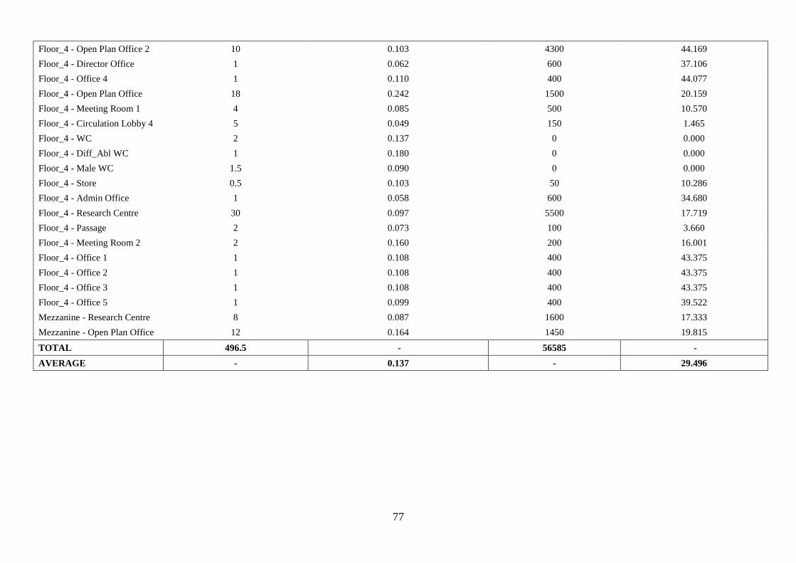
77
Floor_4 - Open Plan Office 2 10 0.103 4300 44.169
Floor_4 - Director Office 1 0.062 600 37.106
Floor_4 - Office 4 1 0.110 400 44.077
Floor_4 - Open Plan Office 18 0.242 1500 20.159
Floor_4 - Meeting Room 1 4 0.085 500 10.570
Floor_4 - Circulation Lobby 4 5 0.049 150 1.465
Floor_4 - WC 2 0.137 0 0.000
Floor_4 - Diff_Abl WC 1 0.180 0 0.000
Floor_4 - Male WC 1.5 0.090 0 0.000
Floor_4 - Store 0.5 0.103 50 10.286
Floor_4 - Admin Office 1 0.058 600 34.680
Floor_4 - Research Centre 30 0.097 5500 17.719
Floor_4 - Passage 2 0.073 100 3.660
Floor_4 - Meeting Room 2 2 0.160 200 16.001
Floor_4 - Office 1 1 0.108 400 43.375
Floor_4 - Office 2 1 0.108 400 43.375
Floor_4 - Office 3 1 0.108 400 43.375
Floor_4 - Office 5 1 0.099 400 39.522
Mezzanine - Research Centre 8 0.087 1600 17.333
Mezzanine - Open Plan Office 12 0.164 1450 19.815
TOTAL 496.5 - 56585 -
AVERAGE - 0.137 - 29.496
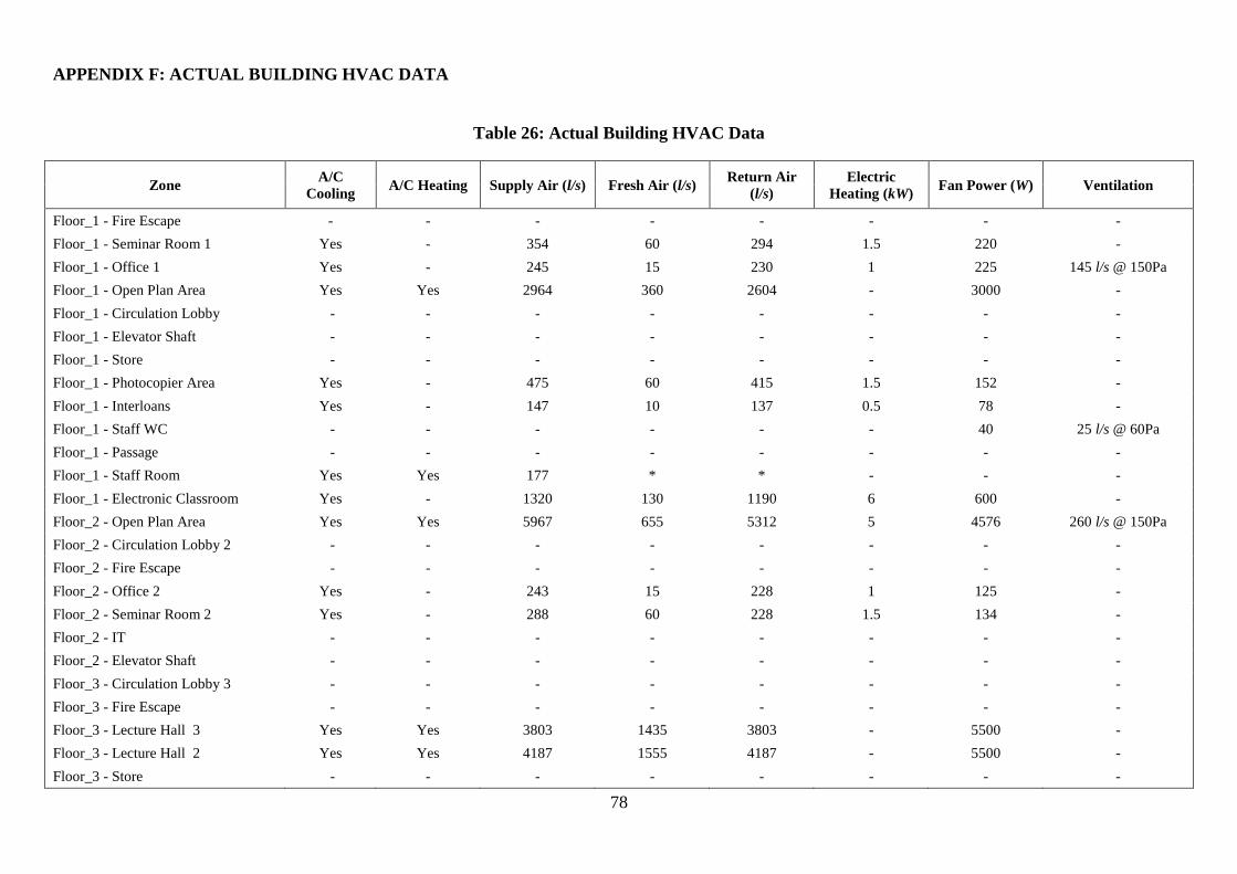
78
APPENDIX F: ACTUAL BUILDING HVAC DATA
Table 26: Actual Building HVAC Data
Zone A/C
Cooling A/C Heating Supply Air (l/s) Fresh Air (l/s)
Return Air
(l/s)
Electric
Heating (kW) Fan Power (W) Ventilation
Floor_1 - Fire Escape - - - - - - - -
Floor_1 - Seminar Room 1 Yes - 354 60 294 1.5 220 -
Floor_1 - Office 1 Yes - 245 15 230 1 225 145 l/s @ 150Pa
Floor_1 - Open Plan Area Yes Yes 2964 360 2604 - 3000 -
Floor_1 - Circulation Lobby - - - - - - - -
Floor_1 - Elevator Shaft - - - - - - - -
Floor_1 - Store - - - - - - - -
Floor_1 - Photocopier Area Yes - 475 60 415 1.5 152 -
Floor_1 - Interloans Yes - 147 10 137 0.5 78 -
Floor_1 - Staff WC - - - - - - 40 25 l/s @ 60Pa
Floor_1 - Passage - - - - - - - -
Floor_1 - Staff Room Yes Yes 177 * * - - -
Floor_1 - Electronic Classroom Yes - 1320 130 1190 6 600 -
Floor_2 - Open Plan Area Yes Yes 5967 655 5312 5 4576 260 l/s @ 150Pa
Floor_2 - Circulation Lobby 2 - - - - - - - -
Floor_2 - Fire Escape - - - - - - - -
Floor_2 - Office 2 Yes - 243 15 228 1 125 -
Floor_2 - Seminar Room 2 Yes - 288 60 228 1.5 134 -
Floor_2 - IT - - - - - - - -
Floor_2 - Elevator Shaft - - - - - - - -
Floor_3 - Circulation Lobby 3 - - - - - - - -
Floor_3 - Fire Escape - - - - - - - -
Floor_3 - Lecture Hall 3 Yes Yes 3803 1435 3803 - 5500 -
Floor_3 - Lecture Hall 2 Yes Yes 4187 1555 4187 - 5500 -
Floor_3 - Store - - - - - - - -

79
Floor_3 - Elevator Shaft - - - - - - - -
Floor_4 - Fire Escape - - - - - - - -
Floor_4 - Open Plan Office 2 Yes Yes 1199 65 1134 - 1100 -
Floor_4 - Director Office Yes Yes 271 20 251 - 134 -
Floor_4 - Office 4 Yes Yes 271 15 256 - 134 -
Floor_4 - Open Plan Office Yes Yes 1070 90 980 - 576 -
Floor_4 - Meeting Room 1 Yes Yes 774 100 674 - 440 -
Floor_4 - Circulation Lobby 4 - - - - - - - -
Floor_4 - WC - - - - - -
180 320 l/s @ 130Pa Floor_4 - Diff_Abl WC - - - - - -
Floor_4 - Male WC - - - - - -
Floor_4 - Store - - - - - - - -
Floor_4 - Admin Office Yes Yes 245 10 235 - 125 -
Floor_4 - Research Centre Yes Yes 3766 188 3578 - 2156 -
Floor_4 - Passage - - - - - - - -
Floor_4 - Meeting Room 2 Yes Yes 238 20 208 - 125 -
Floor_4 - Office 1 Yes Yes 144 15 129 - 78 -
Floor_4 - Office 2 Yes Yes 144 15 129 - 78 -
Floor_4 - Office 3 Yes Yes 144 15 129 - 78 -
Floor_4 - Office 5 Yes Yes 144 15 129 - 78 -
Floor_4 - Elevator Shaft -
- - - - - -
Mezzanine - Research Centre Yes Yes 1003 65 938 - 1100 -
Mezzanine - Director Office -
- - - - - -
Mezzanine - Open Plan Office Yes Yes 1199 65 1134 - 1100 -
Mezzanine - Admin Office - - - - - - -
TOTAL - - 30782 5053 28532 18 27632 -
Note: *) No ventilation data for zone was available at the first design stage.

80
APPENDIX G: CRSES BUILDING ZONES
The new academic building zones which CRSES will occupy are shown in Table
27 below. Some of these zones will however be used by MIH as well, but for a
better overall energy performance assessment was all the overlapping zones
included. The location of these zones is shown in Figure 38, Appendix B.
Table 27: Building zones which CRSES is comprised of.
Floor_4 - Open Plan Office 2
Floor_4 - Director Office
Floor_4 - Office 4
Floor_4 - Open Plan Office
Floor_4 - Meeting Room 1
Floor_4 - WC
Floor_4 - Diff_Abl WC
Floor_4 - Male WC
Floor_4 - Store
Floor_4 - Admin Office
Floor_4 - Passage
Floor_4 - Meeting Room 2
Floor_4 - Office 1
Floor_4 - Office 2
Floor_4 - Office 3
Floor_4 - Office 5
Mezzanine - Director Office
Mezzanine - Open Plan Office
Mezzanine - Admin Office

81
APPENDIX H: OPEN PLAN OFFICE 2 SIMULATION RESULTS
To better understand the actual building energy performance on a zone level, the
Open Plan Office 2 zone on the fourth floor was chosen for further investigation.
Figure 40 below shows a wireframe representation of Open Plan Office 2 with
windows outlined in yellow, doors outlined in blue and openings outlined in
green.
Figure 40: Actual building Open Plan Office 2 zone wireframe
representation.
From Figure 31 and Figure 40 it is evident that the large glazing area of Open
Plan Office 2 on the 113° façade of the actual building will have a large impact on
the early morning solar energy gains. The internal heat gains resulting from this
building fabric design feature is shown in the summer design day (15 January
2002) internal heat balance data of Figure 41 below.
113° Façade

82
Figure 41: Actual building Open Plan Office 2 summer design day internal
gains.
Maximum solar energy gain occurs at 08:00 as depicted in Figure 41 above. This
large heat energy results in a rapid increase in the cooling requirement of the zone.
For the rest of the day, a large and reasonably constant cooling energy load is
required to sustain internal thermal comfort temperatures due to the GSSA-PEB
operational profiles shown in Figure 17 (applicable to this zone on the day the
data depicted in Figure 41 was acquired).

83
Figure 42: Actual building Open Plan Office 2 summer design day fabric and
ventilation performance results.
The Open Plan Office 2 building fabric heat balance simulation data depicted in
Figure 42 above shows the heat retention characteristics of the most significant
building fabric components. An important observation made from this data is the
ability of the internal building floors to release a large amount of stored cooling
energy early in the morning when the large solar energy heat gain shown in Figure
41 occurs. This positive natural energy offset is predominantly attributed to the
large amount of thermal capacitance as a result of the mass, density and specific
heat capacity of concrete in the internal floors.
The internal partitions has less thermal capacitance per unit area than the internal
concrete floors, but because this zone has a large amount of internal partition
surface does the combined thermal capacitance provide a notable positive offset in
heat energy gain.
A further simulation was done on a winter design temperature of 3.8° Celsius to
determine the building fabric performance of Open Plan Office 2. The data
obtained in this simulation is presented in Figure 43 below.
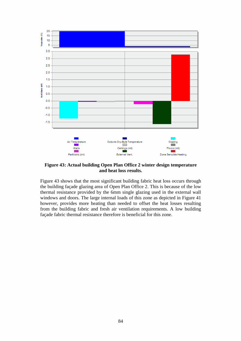
84
Figure 43: Actual building Open Plan Office 2 winter design temperature
and heat loss results.
Figure 43 shows that the most significant building fabric heat loss occurs through
the building façade glazing area of Open Plan Office 2. This is because of the low
thermal resistance provided by the 6mm single glazing used in the external wall
windows and doors. The large internal loads of this zone as depicted in Figure 41
however, provides more heating than needed to offset the heat losses resulting
from the building fabric and fresh air ventilation requirements. A low building
façade fabric thermal resistance therefore is beneficial for this zone.

85
APPENDIX I: SOLAR PHOTOVOLTAIC ROOF ARRAY
The primary design considerations for the PV panel array on the roof of the new
academic building were to use a robust technology within a very limited budget
and ensure that the panels can be mounted flush to the roof. A secondary design
consideration was to design the size and placement of the PV array on the roof
surface such that local shading by the adjacent buildings is minimised. This was
done by analysing the shading effects of the adjacent buildings on the solar
equinox and solstice days. Figure 44 below shows the placement of the PV panel
array on the roof of the new building and the shading created by the surrounding
buildings at 08:00 on the solar equinox day of 20 March.
Figure 44: Plan view of academic building with PV array on roof (black
rectangle).
An analysis of the shading created by the surrounding buildings on the solar
equinox and solstice days revealed that the location of the PV array (shown above
in Figure 44) will receive a very small amount of shading very early in the
mornings and late afternoon. To compensate for this effect a 5% DNI solar
shading factor has been incorporated into the simulation.
The technical specifications of the PV panel array chosen for the new academic
building are defined in Table 28 below.

86
Table 28: PV array specifications.
Solar cell technology used Monocrystalline silicon
PV array panel count 80 panels
PV array dimensions 10.62 m long and 12.64 m wide
PV array area 134.24 m2
PV array tilt angle 10°
Total PV panel array weight 1600 kg(1)
PV panel array cost R 360 000(2)
PV array maximum power rating 16 kW(3)
Inverters for 240 VAC power generation 5 X Solaris 3500 XP 240V
(SAM, 2011)
Note: 1) Only applicable to the panels. 2) Quoted in South African Rand by Mantech Electronics
(2011). 3) Rated at an irradiance level of 1000 W/m2 and an air mass spectrum of 1.5 per cell.
To calculate the total annual PV system energy output, a simulation was done in
the Solar Advisor Model software provided by the NREL (SAM, 2011). The
weather file used in this software to simulate the annual solar irradiance levels
was the same weather file used for simulating the annual building energy
consumption (refer to section 3.2.2). The simulation results are tabulated below in
Table 29 and the monthly energy output is shown below in Figure 45.
Table 29: PV array simulation results.
Total system electrical derate between PV
panel array and 240 VAC inverter output 15%
Total system performance factor 0.76
Total system annual energy output 24 323 kWh
Figure 45: PV array monthly energy output.
0
500
1000
1500
2000
2500
3000
Jan Feb Mar Apr May Jun Jul Aug Sep Oct Nov Dec
Ene
rgy
ou
tpu
t (kWh
)

87
End


