Energy-Efficient Timely Transportation of Long-Haul Heavy ...

IEEE TRANSACTIONS ON INTELLIGENT TRANSPORTATION SYSTEMS, VOL. 19, NO. 7, JULY 2018 2099

Energy-Efficient Timely Transportationof Long-Haul Heavy-Duty Trucks

Lei Deng, Mohammad H. Hajiesmaili, Minghua Chen, Senior Member, IEEE, and Haibo Zeng, Member, IEEE

Abstract— We consider a timely transportation problem wherea heavy-duty truck travels between two locations across thenational highway system, subject to a hard deadline constraint.Our objective is to minimize the total fuel consumption of thetruck, by optimizing both route planning and speed planning. Theproblem is important for cost-effective and environment-friendlytruck operation, and it is uniquely challenging due to its combina-torial nature as well as the need of considering hard deadline con-straint. We first show that the problem is NP-complete; thus exactsolution is computational prohibited unless P = NP. We thendesign a fully polynomial time approximation scheme (FPTAS)to solve it. While achieving highly-preferred theoretical per-formance guarantee, the proposed FPTAS still suffers fromlong running time when applying to national-wide highwaysystems with tens of thousands of nodes and edges. Leveragingelegant insights from studying the dual of the original problem,we design a heuristic with much lower complexity. The pro-posed heuristic allows us to tackle the energy-efficient timelytransportation problem on large-scale national highway systems.We further characterize a condition under which our heuristicgenerates an optimal solution. We observe that the conditionholds in most of practical instances in numerical experiments,justifying the superior empirical performance of our heuristic.We carry out extensive numerical experiments using real-worldtruck data over the actual U.S. highway network. The resultsshow that our proposed solutions achieve 17% (resp. 14%)fuel consumption reduction, as compared with a fastest path(resp. shortest path) algorithm adapted from common practice.

Index Terms— Energy-efficient transportation, timely delivery,route planning, speed planning.

I. INTRODUCTION

IN THE U.S., heavy-duty trucks haul more than 70% of allfreight tonnage [2], and they consume 17.6% of energy in

transportation sector [3, Table 2.8] and contribute to about

Manuscript received May 19, 2016; revised June 5, 2017; acceptedAugust 19, 2017. Date of publication October 3, 2017; date of current versionJune 28, 2018. This work was supported in part by National Basic ResearchProgram of China under Grant 2013CB336700 and in part by the UniversityGrants Committee of the Hong Kong Special Administrative Region, China,Theme-based Research Scheme, under Grant T23-407/13-N. This paper waspresented at the seventh ACM International Conference on Future EnergySystems (ACM e-Energy), Waterloo, ON, Canada, 2016 [1]. The AssociateEditor for this paper was P. Ioannou. (Corresponding author: Lei Deng.)

L. Deng and M. Chen are with the Department of Information Engi-neering, The Chinese University of Hong Kong, Hong Kong (e-mail:[email protected]; [email protected]).

M. H. Hajiesmaili is with the Department of Electrical and ComputerEngineering, Johns Hopkins University, Baltimore, MD 21218 USA (e-mail:[email protected]).

H. Zeng is with the Department of Electrical and Computer Engineering,Virginia Tech, Blacksburg, VA 24061 USA (e-mail: [email protected]).

This paper has supplementary downloadable material available athttp://ieeexplore.ieee.org., provided by the author.

Color versions of one or more of the figures in this paper are availableonline at http://ieeexplore.ieee.org.

Digital Object Identifier 10.1109/TITS.2017.2749262

5% of the greenhouse gas emission [4]. Fuel cost is thelargest operating cost (34%) of truck owners/operators [5],and reducing fuel consumption is critical for cost-effective andenvironment-friendly heavy-duty truck operations.

Currently there are mainly two lines of efforts to reduce fuelconsumption of heavy-duty trucks. The first line is to operatewith more fuel efficient trucks, from better designs for engines,drivetrains, aerodynamics, and tires [6]–[8], to better manage-ment of truck parts such as maintaining optimal tire pres-sures [9]. The second line is to operate heavy-duty trucks moreeconomically. This explores several possibilities, e.g., reducingidling energy consumption [10], platooning more than oneheavy-duty trucks [11], [12], route planning [13]–[15], andspeed planning [16]–[19]. In this paper, we focus on route andspeed planning. Different routes could have different mileages,levels of congestion, road grades, and surface types, etc., all ofwhich would largely affect the fuel consumption. Real-worldstudies [15] show that choosing a more efficient route for aheavy-duty truck can improve its fuel economy by 21%. Speedplanning is another well recognized approach to effectivelyreduce fuel consumption. Different running speed could leadto different fuel economy. For a vehicle with certain weightrunning on a road, normally there is a most fuel-efficientspeed. When the running speed is below or above the mostfuel-efficient speed, the fuel economy will be degraded. As arule of thumb for truck operations on highway, every one mileper hour (mph) increase in speed (above the most fuel-efficientspeed) incurs about 0.14 mile per gallon (mpg) decrease in fueleconomy [18], [19].

However, operating at low speed may result in excessivetravel time and the goods carried by the truck cannot bedelivered on time. We remark that timely delivery is criticalfor truck operators [20], [21]. As estimated by the U.S.Federal Highway Administration (FHWA) in [20], unexpecteddelay can increase freight cost by 50% to 250%. Multiplereasons can explain the importance of timely delivery. First,some freight goods are perishable, such as food [22], whichdefinitely require timely delivery. Second, to ensure customers’satisfaction, some companies, e.g., Amazon, may have aservice-level agrement (SLA) with users, under which thedelivery delay is guaranteed [23]. Finally, violating scheduleddelay can introduce difficulties for global logistic decisionsand even increase the uncertainty and inefficiency of supplychains [20]. Overall, it is crucial to ensure timely goodsdelivery for truck operators, and considering timely deliveryin fuel cost minimization poses a unique challenge.

Motivated by the above observations, in this paper, westudy the problem of energy-efficient timely transportation

1524-9050 © 2017 IEEE. Personal use is permitted, but republication/redistribution requires IEEE permission.See http://www.ieee.org/publications_standards/publications/rights/index.html for more information.

2100 IEEE TRANSACTIONS ON INTELLIGENT TRANSPORTATION SYSTEMS, VOL. 19, NO. 7, JULY 2018

TABLE I

COMPARISONS OF OUR STUDY AND EXISTING WORKS ON PERFORMANCE OPTIMIZATION IN VARIOUS TRANSPORTATION SYSTEMS WITH DELAY TAKENINTO CONSIDERATION. HERE RSP STANDS FOR RESTRICTED SHORTEST PATH PROBLEM, VRPTW STANDS FOR VEHICLE ROUTING PROBLEM

WITH TIME WINDOWS, AND BSP STANDS FOR BI-OBJECTIVE SHORTEST PATH PROBLEM

TABLE II

COMPARISONS OF OUR WORK AND EXISTING WORKS ON

ENERGY-EFFICIENT HEAVY-DUTY TRUCK OPERATION

for heavy-duty trucks. We aim to minimize the heavy dutytruck’s fuel consumption while satisfying a hard deadlineconstraint, under which we take both route planning andspeed planning into account to exploit complete design spaceof reducing fuel consumption. Since heavy-duty trucks aremainly operated for long-haul delivery and most of time run onhighways [3, Table 5.2 and Fig. 5.1], we focus our model ontheir operation in the highway transportation network system.We summarize our contributions in the following.

� We formulate an energy-efficient timely transportationproblem of minimizing the fuel consumption subject to ahard deadline constraint for a heavy-duty truck running ona highway transportation network, with design spaces of bothroute planning and speed planning in Sec. II. To the best of ourknowledge, as compared to existing works on energy-efficientheavy-duty truck operation [16], [17], [37], our work is thefirst one that simultaneously considers route planning, speedplanning, and hard deadline (see Tab. II).

� We show that our problem is NP-Complete andthen design a fully polynomial time approximationscheme (FPTAS) in Sec. III to solve our problem. Theproposed FPTAS attains an approximation ratio of (1 + ε)with a network-size induced complexity of O(mn2/ε2),where m and n are the numbers of nodes and edges,respectively.

� While achieving highly-preferred theoretical performanceguarantee, the proposed FPTAS still suffers from long run-ning time when applying to national-wide highway systemswith tens of thousands of nodes and edges. In Sec. IV, by

leveraging elegant insights from studying the dual of theoriginal problem, we design a fast heuristic solution withO(m + n log n) complexity. The proposed heuristic schemeallows us to tackle the energy-efficient timely transportationproblem on large-scale national highway systems. We furthercharacterize a condition under which our heuristic generatesan optimal solution. We observe that the condition holds inmost of the practical instances in numerical experiments inSec. V, justifying the superior empirical performance of ourheuristic.

� We carry out extensive numerical experiments using real-world truck data over the U.S. highway network in Sec. V.The results show that our proposed solutions achieve 17%(resp. 14%) fuel consumption reduction, as compared toa fastest path (resp. shortest path) algorithm adapted fromcommon practice. The amount of fuel consumption saving isenough to power up more than 90% of the entire transportationsector in New York State [38].

Comparison with existing works on energy-efficientheavy-duty truck operation. There are a large number ofworks focusing on energy-efficient heavy-duty truck operation,e.g., [16], [17], [37]. But to the best of our knowledge,our work is the first one that simultaneously considers routeplanning, speed planning, and hard deadline (see Tab. II).

Comparison with existing works on performance opti-mization in various transportation systems with delaytaken into consideration. Theoretically, we also comparethe problem studied in our work with other related problemsstudied in existing works in Tab. I. First, our energy-efficienttimely transportation problem is a generalized version ofRestricted Shortest Path problem (RSP) [24]–[26], with anextra design space of speed planning. Therefore, we generalizethe FPTAS design and the dual-based design of RSP toour problem. Second, for the well-studied Vehicle RoutingProblem with Time Windows (VRPTW) [27]–[30], if we onlyconsider one vehicle and one customer with departure dead-line, then it becomes the RSP problem, which is a special caseof our problem without speed planning. Third, our problemcan be regarded as a special case of the studied problems

DENG et al.: ENERGY-EFFICIENT TIMELY TRANSPORTATION OF LONG-HAUL HEAVY-DUTY TRUCKS 2101

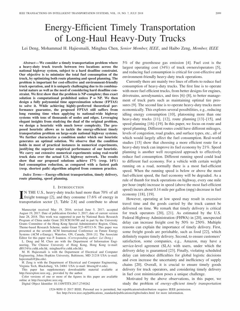
Fig. 1. System model.

in [31] and [32] under different contexts from our focus ontrucks, where both route planning and speed planning areconsidered. However, [31], [32] do not prove the hardness ofthe problem and only propose a heuristic algorithm withoutperformance guarantee to solve the problem. The heuristicalgorithm in [31] uses the column generation approach but ter-minates in certain iterations, and the heuristic algorithm in [32]is based on a multi-start local search approach, both of whichcould incur high complexity and do not have performanceguarantee. The performance of these generic approaches canbe quite unsatisfactory in some specific problems. For exam-ple, column generation approach suffers from slow conver-gence and thus terminating in certain iterations could producea solution far away from the optimal one [39], [40], andmulti-start local search could also get trapped in a bad localoptimum [41]. Our work, instead, shows that our studied prob-lem is NP-complete, and proposes an FPTAS and a heuristicalgorithm with characterizing an optimality condition to solvethe problem. Our numeric results in Sec. V demonstrate theexcellent performance of our solutions in practical scenarios.We also explicitly show that the time complexity of theFPTAS and the heuristic is polynomial in the problem size.Finally, another related problem is the Bi-objective Short-est Path problem (BSP) [33]–[36], which needs to find allPareto-optimal paths to simultaneously minimize the travelcost and travel time. BSP is different from our problem inthat it regards the travel time as one objective instead of aconstraint to satisfy and it does not have the design space ofspeed planning.

Due to the space limitation, all proofs are included in thesupplementary materials.

II. MODEL AND PROBLEM FORMULATION

A. System Model

Consider a highway transportation network as exemplifiedin Fig. 1. We model it as a directed graph G = (V, E),where V is the vertex/node set and E is the edge/road set.We define n � |V| as the number of nodes and m � |E |as the number of edges. For each edge e ∈ E , we denoteDe > 0 as its distance (unit: mile), and Rlb

e > 0 (resp.Rub

e ≥ Rlbe ) as its minimum (resp. maximum) speed (unit:

mph). (Governments usually set the maximum speed for allhighways and the minimum speed for some highways. For thesake of both safety and fuel efficiency, lower speed limits than

passenger cars may be applied to large commercial vehicleslike heavy-duty trucks and buses.) Now consider a long-haulheavy-duty truck at time 0 who aims to ship cargos from asource node s ∈ V to a destination node d ∈ V . The goal isto minimize the energy/fuel1 consumption subject to a harddeadline requirement T > 0 (unit: hour).

Fuel consumption and travel delay are usually in conflictwith each other, both of which are related to the speedprofile of the truck. High travel speed obviously decreasesthe travel delay, but it can also increase the fuel consumptionsignificantly [18], [19]. To analyze the performance tradeoffbetween energy and delay, we need to model the relationshipbetween the fuel consumption and the travel speed. There arean intensive number of such models (see a survey in [42]).In this paper, we use the instantaneous fuel consumptionmodel [42], [43] which generally depends on three factors:(i) static vehicle/road/environment properties, (ii) instanta-neous acceleration/deceleration, and (iii) instantaneous speed.As we consider a specific vehicle running over a spe-cific network, static vehicle/road/environment properties arefixed, and thus we model them as fixed parameters in ourfuel consumption model. We further neglect the effects ofinstantaneous acceleration/deceleration based on the follow-ing two observations. First, as shown in [44] and [45] andour results in Lemma 1, running at a constant speed ismost fuel-economic on a road segment with homogeneousgrade and road/environment conditions. Thus, it is reasonableto ignore the effects of acceleration/deceleration inside anyroad segment (with homogeneous grade and road/environmentconditions). Second, while a truck may involve accelera-tion/deceleration when switching from one road segment toanother road segment, the acceleration/deceleration distanceis negligible as compared to the length of road segments. Forexample, as shown in [46], the heavy-duty truck can acceleratefrom zero speed to 31mph in just 500 feet, while the averagelength of highway road segments is 3.26 miles, according toour study of the U.S. national highway data (see Tab. IV).Thus, it is also reasonable to ignore the effects of accelera-tion/deceleration during road segment switch. With the abovejustification, in this paper, we assume that the instantaneousfuel consumption is a function of the instantaneous speed.

We thus define fe : [Rlbe , Rub

e ] → R+ as the (instantaneous)

fuel-rate-speed function of the truck running on edge e:if the vehicle’s speed on edge e is re (unit: mph), the fuelconsumption rate is fe(re) (unit: gallons per hour (gph)),and then the total fuel consumption for driving time τ (unit:hour) with the constant speed re is fe(re) · τ (unit: gallon).Since many existing models [43], [47]–[50] use polynomialfunctions to model the fuel consumption which are alsostrictly convex in a reasonable speed limit region, in thispaper, we assume that fe(·) is a polynomial function andis strictly convex2 over [Rlb

e , Rube ]. This assumption also

holds in the physical interpretation of fuel-rate-speed functionas shown in Append. A in the supplementary materials,

1We interchangeably use fuel and energy in this paper.2The strict convexity can be relaxed to convexity. For simplicity, we use

the strict convexity in this paper.


and is further verified in our simulation using real-world data(see Fig. 5(a)).

B. Problem Formulation

We consider two design spaces: path selection (routeplanning) and speed optimization (speed planning). For pathselection, we define a binary variable xe for any e ∈ E ,

xe ={

1, Edge e is on the selected path;

0, otherwise.(1)

For the speed optimization, the truck needs to determine aspeed profile (speeds at all travel time) over any selectededge. This is a functional variable, but the convexity of fuel-rate-speed function can simplify the speed profile significantlybased on the following lemma.

Lemma 1: For any edge e, if the travel time te is given,i.e., the truck must pass edge e with exactly te hours, then theoptimal speed profile to minimize the fuel consumption is tomaintain constant speed De/te during the whole trip.

Proof: See Append. B in the supplementary materials.Lemma 1 shows that for any edge, any non-constant speed

profile is dominated by another constant speed profile interms of fuel consumption without sacrificing the delay per-formance. Therefore, without loss of optimality, the truck onlyneeds to follow a constant speed for any edge. As explainedin Sec. II-A, since we consider a long-haul highway scenario,we will ignore the speed transition period between two adja-cent edges. Thus, for the speed optimization, we consider thetravel time te > 0 over each edge e as the design variable,which equivalently implies a constant speed De/te over e.We then define a fuel-time function ce(·) for each road e,

ce(te) � te · fe(De

te), (2)

which is the total fuel consumption for the truck travelingedge e with travel time te.

By vectorizing our decision variables as x � {xe : e ∈ E}and t � {te : e ∈ E}, now we are ready to formulate our PAthselection and Speed Optimization (PASO) problem,

PASO: minx∈X ,t∈T

∑e∈E

xe · ce(te) (3)

s.t.∑e∈E

xete ≤ T, (4)

In PASO, set X restricts that one and only one s − d pathis selected, defined as

X � {x : xe ∈ {0, 1},∀e ∈ E, and∑e∈out(v)

xe −∑

e∈in(v)

xe = 1{v=s} − 1{v=d},∀v ∈ V},

where 1{·} is the indicator function, in(v) � {(u, v) :(u, v) ∈ E} is the set of incoming edges of node v ∈ V ,out(v) � {(v, u) : (v, u) ∈ E} is the set of outgoing edges ofnode v. Set T captures the speed limits of all roads, defined as

T � {t : t lbe ≤ te ≤ tub

e ,∀e ∈ E},

where t lbe � De

Rube

and tube � De

R lbe

are the minimum and maxi-mum travel time due to the speed limits on edge e, respectively.Constraint (4) is to satisfy the hard deadline requirement.Objective (3) is to minimize the total fuel consumption overthe selected path.

Note that one major difficulty of our problem PASO is thatthe route planning and the speed planning are coupled witheach other and thus we need to tackle them simultaneously.

C. Complexity Hardness

PASO has both integer variables and continuous variables.Thus it is worth understanding its hardness first. It turns outthat a special case of PASO is the well-known RestrictedShortest Path (RSP) problem [24], [25]. In RSP, a directedgraph is given where each edge has a fixed travel time andtravel cost, and the goal is to find a minimum-cost pathsubject to a hard path deadline requirement. Clearly, ourproblem PASO generalizes RSP where we allow a varyingedge cost and edge time because of the design space of speedoptimization. Since RSP is NP-Complete [25], we can thuseasily prove that our problem PASO is also NP-Complete.

Theorem 1: PASO is NP-Complete.Proof: We can prove it by setting Rlb

e = Rube to an

appropriate value for each edge e in PASO, and using theresult that RSP is NP-Complete [25].

Theorem 1 shows that exact solution is computational pro-hibited unless P=NP. In this paper, we thus seek approximatebut efficient solutions to PASO.

D. Preprocessing and Some Notations

We first check the feasibility of our problem PASO. We canuse the shortest path algorithm where each edge e has cost t lb

eto find the fastest path. If the travel time of the fastest path islarger than the deadline requirement T , PASO is infeasible.In the rest of this paper, we thus assume that the deadlineconstraint T is at least the travel time of the fastest path suchthat the problem is feasible.

We then analyze properties of the fuel-time function ce(·).Lemma 2: ce(te) is strictly convex over [t lb

e , tube ]. Also,

there exists a point te ∈ [t lbe , tub

e ]3 such that ce(te) is firststrictly decreasing over [t lb

e , te] and then strictly increasingover [te, tub

e ].Proof: See Append. C in the supplementary materials.

Based on Lemma 2, we can easily prove that the traveltime over edge e, i.e., te, in any optimal solution of PASOmust be in the region [t lb

e , te]. Otherwise, we can decrease thetravel time from te to te and at the same time decrease thefuel consumption, which violates the optimality of te. Thus,without loss of optimality, we can reset the travel time limitfrom [t lb

e , tube ] to [t lb

e , te], which equivalently implies that wereset the speed limit from [Rlb

e , Rube ] to [De/te, Rub

e ]. Aftersuch preprocessing, in the rest of the paper, ce(te) can beassumed to be strictly convex and strictly decreasing overte ∈ [t lb

e , tube ] without loss of optimality.

In the rest of the paper, define an s − d path p as the set ofall edges over p and t p � {te : e ∈ p} as the corresponding

3Note that te can be on the boundary.


travel time set. Moreover, we define c(p, t p) �∑

e∈p ce(te)as the fuel consumption of path p with travel time set t p , andOPT as the optimal value of PASO.

Next, we will propose a fully polynomial time approxima-tion scheme (FPTAS) in Sec. III and a fast dual-based heuristicscheme in Sec. IV to solve our problem PASO.

III. AN FPTAS FOR PASO

Since PASO generalizes RSP, which is well-known to havean FPTAS [24], [51], it is natural to ask whether we canextend RSP’s FPTAS for our problem PASO. In this section,by carefully tackling the difference between PASO and RSP,we “reformulate” PASO such that we can adapt RSP’s FPTASto construct an FPTAS for PASO. More specifically, in thissection, we propose an approximation scheme (Algorithm 3)such that for any given ε ∈ (0, 1), it can find a (1 + ε)-approximate solution in the sense that the solution is feasibleand the corresponding fuel consumption is at most (1+ε)OPT,and the time complexity is polynomial in both the problemsize and 1

ε .The essence of RSP’s FPTAS [24], [51] is a test procedure.

For any input value S > 0 and any input accuracy parameterδ > 0, the test procedure can “approximately” compare Sand the optimal value OPT in the sense that it can tell eitherOPT > S or OPT ≤ (1 + δ)S in polynomial time. Based onthis test procedure, starting with some arbitrary lower boundLB and upper bound UB for OPT, a binary search scheme isdesigned [24], [51] to exponentially narrow down the boundinginterval [LB, UB] and finally a (1 + ε)-approximate solutionis outputted.

To solve our problem PASO, we adapt RSP’s FPTAS bydesigning our own test procedure. In RSP, [24] and [51] usethe rounding and scaling technique, where each fixed edgecost is rounded into certain (polynomial) number of cost levelscontrolled by the accuracy parameter δ. As we only requirean “approximate” comparison, rounding into certain numberof cost levels is enough to perform such a task. However, asopposed to a fixed edge cost in RSP, in PASO each edge hasa fuel-time function. Hence, instead of rounding a fixed costin RSP, we quantize the continuous fuel-time function ce(·)into another staircase fuel-time function ce(·) according to theinput value S and the input accuracy parameter δ, which can befurther characterized by a polynomial number of representativepoints. We then prove that such quantization can perform the“approximate” comparison.

Later on we will describe our algorithms in a bottom-up fashion. We first describe the quantizing procedure(Algorithm 1) in Sec. III-A. Then we present our own test pro-cedure (Algorithm 2) which invokes Algorithm 1 in Sec. III-B.Finally, we describe the whole FPTAS (Algorithm 3) whichinvokes Algorithm 2 in Sec. III-C.

A. Quantizing Fuel-Time Function

For any input value V > 0 and N ∈ Z+, we quantize the

edge-e fuel-time function ce(te) to be

ce(te) � min

{⌊ce(te)

V

⌋+ 1, N

}, ∀te ∈ [t lb

e , tube ]. (5)

Fig. 2. An example for quantizing ce(·).

Since we have assumed that ce(te) is strictly decreasingin Sec. II-D, ce(te) thus becomes a staircase function withat most N stairs. During the quantization, parameter V is tocontrol the accuracy, which is the vertical span of each stair.Larger V means rougher quantization and lower accuracy butsmaller complexity. Parameter N is to control the maximumnumber of stairs. Since ce(te) could take an arbitrarily largevalue, the number of stairs could be unbounded, which def-initely incurs high complexity. To design a polynomial timetest procedure where we only need to perform an “approxi-mate” comparison, we truncate ce(te) by putting a ceil V N .This truncation is sufficient for use in the test procedure(see Sec. III-B). Clearly, ce(te) is a quantized and truncatedversion of ce(te). An example is shown in Fig. 2. Here weset V = 20, N = 4. Thus, each stair spans 20 and ce(te) istruncated by the ceil V N = 80. The resulting curve ce(te) isa non-increasing staircase function, which jumps from 4 to 3at te = 1.8 and jumps from 3 to 2 at te = 2.8.

Moreover, since ce(te) is a staircase function and onlytakes integer values, we can use an N-dim vector τ e torepresent it without any information loss. We define it asτ e � (τ 1

e , τ 2e , · · · , τ N

e ) where τ ie is the minimum travel time

over [t lbe , tub

e ] such that ce(·) = i and is defined as nan ifce(·) = i has no solution. For the example in Fig. 2, we haveτe = (τ 1

e , τ 2e , τ 3

e , τ 4e ) = (nan, 2.8, 1.8, 1).

We call (τ ie , i) the i -th representative point of ce(·). Thus

ce(·) is characterized by at most N representative points,which will play a key role in our test procedure in Sec. III-B.We summary the quantizing procedure QUANTIZE(e, V , N)in Algorithm 1. The basic idea is to first find the range of thestair levels, i.e., [nmin, nmax] and then find τ i

e for any level iin this range by solving an equation ce(te) = i V .

1) Time Complexity: (i) When nmin = nmax (e.g., iftube = t lb

e ), the loop in lines 7-12 will not be executed.Thus, the total complexity of QUANTIZE(e, V , N) is O(N)due to the initial loop in lines 1-3. (ii) When nmin < nmax,we need to solve an equation for each i in the range[nmin, nmax − 1] as shown in line 8. Since we have assumedthat ce(te) is a strictly decreasing function, we can usea binary search to solve this equation, which has time

complexity O(

log⌈

tube −t lb

etol

⌉)where tol is the tolerance level

for termination. The total complexity of QUANTIZE


(e, V , N) is O(

N + (nmax − nmin) log⌈

tube −t lb

etol

⌉)=

O(

N + N log⌈

tube −t lb

etol

⌉)= O

(N log

(2⌈

tube −t lb

etol

⌉)).

To unify the expression of time complexity forboth (i) and (ii), we define

ξe � max

{2, 2

⌈tube − t lb

e

tol

⌉},

then the complexity of QUANTIZE(e, V , N) is O(N log ξe).Also, if we define

ξ � maxe∈E

ξe, (6)

then the complexity of QUANTIZE(e, V , N) is O(N log ξ) forany e ∈ E .

Algorithm 1 A Quantizing Procedure QUANTIZE(e, V , N)

1: for i = 1, 2, · · · , N do2: Set τ i

e = nan3: end for4: Set nmin = ce(tub

e ) = min{� ce(tube )

V � + 1, N}5: Set nmax = ce(t lb

e ) = min{� ce(t lbe )

V � + 1, N}6: Set τ nmax

e = t lbe

7: for i = nmin, nmin + 1, · · · , nmax − 1 do8: Solve the equation ce(te) = i V over te ∈ [t lb

e , tube ]

9: if the equation has a solution te then10: Set τ i

e = te11: end if12: end for13: return τ e = (τ 1

e , τ 2e , · · · , τ N

e )

B. The Test Procedure

As introduced above, the test procedure should “approx-imately” compare S and the optimal value OPT such thatit can answer either OPT > S or OPT ≤ (1 + δ)S inpolynomial time. Inspired by [51], which improves the FPTASof RSP in [24], we adopt a more powerful test procedure,denoted by TEST(L, U, δ). It can answer either OPT > U orOPT ≤ U +δL. Clearly, if we set L = U = V , TEST(S, S, δ)can answer either OPT > S or OPT ≤ (1+δ)S, which exactlycompletes the “approximate” comparison. The reason to adopta more powerful test procedure, similar to [51], is that we willalso use it to finally output a (1 + ε)-approximate solution.We will discuss it soon in Sec. III-C.

The details of TEST(L, U, δ) are shown in Algorithm 2.As we mentioned before, the major difference between ourproblem PASO and the existing problem RSP is that PASOhas a continuous fuel-time function for each edge instead ofa fixed cost. Thus, different from the test procedure for RSP(see [51, Fig. 1]), we have a step to invoke the quantizingprocedure (Algorithm 1) to quantize the fuel-time function, asshown in lines 3-5 in Algorithm 2. More importantly, since ourtest procedure TEST(L, U, δ) aims to check either OPT > Uor OPT ≤ U + δL, roughly speaking, we do not need toquantize the portion of each fuel-time function with high fuel

cost, i.e., larger than U + δL. Hence, to ensure polynomialtime complexity eventually, we put a ceil V (N + 1) for ce(te)as shown in line 4 of the algorithm, where V and N areappropriately set such that V (N + 1) ≥ U + δL.

After such quantization, the fuel-time function ce(te) foreach edge e consists of at most N + 1 representativepoints. Therefore, conceptually we can construct a new graphG = (V, E). Each edge e ∈ E in the original graph correspondsto at most N + 1 edges in the new graph E . For each edgee ∈ E , the edge cost ce is a positive integer, as shown in (5).This is exactly an RSP problem. Therefore, the remainingsteps follow the test procedure for RSP on the new graph G.Specifically, since each edge e ∈ E has at most N +1 possiblecost values all of which are positive integers (each edge ein the new graph E has a positive integer cost), we can usedynamic programming to complete such test. Similar to [24]and [51], we define gv (c) as the minimum path travel timeamong all s − v paths whose path cost is at most c ∈ Z

+, anddefine gv(c) = ∞ if no such path. The optimality condition(or Bellman’s equation) becomes, for any c = 1, 2, · · · ,

gv (c) = min{gv(c − 1),

minu,i:e=(u,v)∈E,i=1,··· ,N,τ i

e =nan{gu(c − i) + τ i

e }} (7)

which is shown in line 10 in Algorithm 2. Since we onlyneed to answer either OPT > U or OPT ≤ U + δL, wedo not have to process large c. Instead, iterating c from 1to N is enough for us to complete this task. This dynamicprogramming procedure is shown in lines 6-15 of Algorithm 2.

In PASO, we should carefully design the quantizing andthe dynamic programming procedures jointly to guaranteeperformance, as shown in the following lemmas, which arethe counterparts to Lemma 2 and Lemma 3 for RSP in [51].

Algorithm 2 A Test Procedure TEST(L, U, δ)

1: Set V = Lδn+1

2: Set N = �UV � + n + 1

3: for e ∈ E do4: Get τ e = QUANTIZE(e, V , N + 1)5: end for6: Set gs(c) = 0, ∀c = 0, 1, · · · , N7: Set gv(0) = ∞, ∀v = s, v ∈ V8: for c = 1, 2, · · · , N do9: for v ∈ V do

10: Set gv (c) according to (7)11: end for12: if gd(c) ≤ T then13: return the corresponding path p and travel time set

t p = {te : e ∈ p}14: end if15: end for16: return FAIL

Lemma 3: If Algorithm 2 returns a path p and travel timeset t p , then we have

OPT ≤ c(p, t p) ≤ U + Lδ. (8)


Proof: See Append. D in the supplementary materials.Lemma 4: If U ≥ OPT, then Algorithm 2 must return a

feasible path p and travel time set t p , which satisfy

c(p, t p) ≤ OPT + Lδ. (9)

Proof: See Append. E in the supplementary materials.Lemma 5: If Algorithm 2 returns FAIL, then we have

OPT > U. (10)

Proof: This directly follows Lemma 4.Our test procedure either returns a path p and travel time

set t p in line 13, which implies that OPT ≤ U + Lδ fromLemma 3, or returns FAIL in line 16, which implies OPT > Ufrom Lemma 5. Therefore, Lemma 3 and Lemma 5 justify thatour test procedure (Algorithm 2) completes the “approximate”comparison, i.e., answers either OPT > U or OPT ≤ U + Lδ.

Thus, for the purpose of the test procedure, Lemma 3 andLemma 5 are enough. However, we present Lemma 4, whichis stronger than Lemma 5, to provide a sufficient conditionsuch that our test procedure returns a path p and travel timeset t p . We will use Lemma 4 shortly in Sec. III-C to finallyoutput a (1 + ε)-approximate solution.

1) Time Complexity: The quantizing procedures for alledges in lines 3-5 require O(m N log ξ). The dynamic pro-gramming procedure in lines 6-15 requires O(m N2). SinceN = �U

V � + n + 1 = �UL · n+1

δ � + n + 1 = O(UL · n

δ + n), thetotal time complexity of Algorithm 2 is O(m N log ξ+m N2) =O(m(U

L · nδ + n) log ξ + m(U

L · nδ + n)2).

C. The Proposed FPTAS

Based on our own test procedure (Algorithm 2), we thenfollow the FPTAS for RSP in [51, Fig. 2] by replacing its testprocedure with ours. For completeness, we present the FPTASin Algorithm 3 and explain it with the following three steps.

Algorithm 3 An FPTAS1: Get a lower bound LB and upper bound UB for OPT2: Set BL = LB3: Set BU = UB4: while BU

BL> 16 do

5: S = √BL · BU

6: Call TEST(S, S, 1)7: if TEST(S, S, 1) returns FAIL then8: Set BL = S9: else

10: Set BU = 2S11: end if12: end while13: Call TEST(BL, BU , ε)

Step 1 (line 1): To initialize the bound interval, we needto first obtain a lower bound LB and an upper bound UBfor the optimal value OPT. Define that the minimum single-edge fuel cost is Clb � mine∈E ce(tub

e ) and the maximumsingle-edge fuel cost is Cub � maxe∈E ce(t lb

e ). Simply, wecan use the minimum single-edge fuel consumption Clb as

Fig. 3. Binary search (Step 2) of Algorithm 3.

the lower bound LB and use the maximum single-path4 fuelconsumption nCub as the upper bound UB. Also, in Sec. IV,we will propose a heuristic scheme which can always outputa set of LB and UB.

Step 2 (lines 2-12): Using the initial lower bound LBand upper bound UB, we design a binary search scheme,which repeatedly invokes our test procedure (Algorithm 2)to exponentially narrow down the bound interval [BL, BU ]until BU /BL ≤ 16. The binary search step is visualized inFig. 3. Note that we always keep BL as a lower bound andBU as an upper bound for OPT. Whenever BU/BL > 16, weinput the geometric mean S = √

BL · BU and δ = 1 to thetest procedure, as shown in lines 5 and 6. If TEST(S, S, 1)returns FAIL, then according to Lemma 4, we must haveS < OPT. In this case, we reset the lower bound BL to be Sin line 8. Otherwise, TEST(S, S, 1) returns a feasible path pand travel time set t p. According to Lemma 3, we must haveOPT ≤ S + δS = 2S. We reset the upper bound to be 2S inline 10. It can be easily shown that this binary search returnsa lower bound BL and an upper bound BU for OPT such thatBU/BL ≤ 16 in O(log log UB

LB ) iterations.Step 3 (line 13): When BU

BL≤ 16, we call our test procedure

again but we use L = BL and U = BU and δ = ε. SinceBU ≥ OPT, according to Lemma 4, TEST(BL, BU , ε) mustreturn a feasible path p and travel time t p such that

c(p, t p) ≤ OPT + εBL ≤ OPT + εOPT = (1 + ε)OPT.

Therefore, we get a (1 + ε)-approximate solution to PASO.1) Time Complexity: Step 1 requires O(m) to get an initial

lower bound LB and upper bound UB. Step 2 invokes thetest procedure O(log log UB

LB ) times and each invoke takesO(mn log ξ + mn2) time by using L = U = S and δ = 1.Thus Step 2 takes O((mn log ξ + mn2) log log UB

LB ). Step 3

also invokes the test procedure, and it takes O(mn log ξε + mn2

ε2 )

time by using δ = ε < 1 and O(UL ) = O( BU

BL) = O(1)

because BUBL

≤ 16 = O(1). Here we can also see why

we need to use a binary search to obtain BUBL

≤ 16 in

Step 2. This is because BUBL

= O(1) ensures polynomial

time complexity in Step 3. Therefore, the total complexity isO((mn log ξ + mn2) log log UB

LB + mn log ξε + mn2

ε2 ).

4A simple path can have at most n edges.


We summarize our results for the approximate scheme inthe following theorem.

Theorem 2: Algorithm 3 returns a (1 + ε)-approximatesolution for PASO in time O((mn log ξ + mn2) log log UB

LB +mn log ξ

ε + mn2

ε2 ). In addition, under our assumption that anyedge-e fuel-rate-speed function fe(·) is a polynomial function(see Sec. II-A), when we use LB = Clb and UB = nCub whereClb � mine∈E ce(tub

e ) and Cub � maxe∈E ce(t lbe ) = ce1(t

lbe1

),we have log log UB

LB = max{O(log log n), O(Ie1 )} where Ie1 isthe input size of all parameters of edge e1. Thus, Algorithm 3has time complexity polynomial in the input size of theproblem PASO and 1

ε and therefore is an FPTAS.Proof: See Append. F in the supplementary materials.

Although we generalize the FPTAS design fromRSP to PASO, such an FPTAS (Algorithm 3) still hashigh complexity for a large-scale highway network withtens of thousands of nodes and edges. In the next section,we propose a heuristic scheme with substantially lowercomplexity.

IV. A FAST DUAL-BASED HEURISTICIn this section, we present a heuristic scheme for our prob-

lem PASO based on Lagrangian relaxation. Such a heuristicscheme, as we will show later in Sec. IV-C, runs much fasterthan the FPTAS (Algorithm 3). Also, it always outputs a lowerbound LB and an upper bound UB on OPT, which implementsStep 1 in Algorithm 3. Moreover, in most practical scenariosas shown in Sec. V, this heuristic scheme outputs an optimal(or at least near optimal) solution, i.e., LB = UB = OPT(or at least LB ≈ OPT ≈ UB).

A. Lagrangian Relaxation and Dual Problem

In our problem PASO, since the hard deadline constraint (4)couples path selection variable x with speed optimizationvariable t, we relax it and introduce a Lagrangian dual variableλ ≥ 0, which can be interpreted as a (per-unit) delay price overthe entire network.

Based on such relaxation, we can get the correspondingLagrangian,

L(x, t, λ) �∑e∈E

xe · ce(te) + λ(∑e∈E

xete − T )

=∑e∈E

xe · (ce(te) + λte) − λT, (11)

and the corresponding dual function is defined as D(λ) �minx∈X ,t∈T L(x, t, λ). Then the dual problem of PASO isformulated as

(PASO-Dual) maxλ≥0

D(λ)

B. Obtain Dual Function

Before we solve the dual problem, let us first show how toobtain the dual function for a given λ as follows,

D(λ) = minx∈X ,t∈T

L(x, t, λ)

= −λT + minx∈X ,t∈T

∑e∈E

xe · (ce(te) + λte)

(E1)= −λT + minx∈X

[mint∈T

∑e∈E

xe · (ce(te) + λte)

]


∑e∈E

xe · mint lbe ≤te≤tub

e

(ce(te) + λte)


∑e∈E

xe · [ce(t∗e (λ)) + λt∗e (λ)

](E4)= −λT + min

x∈X∑e∈E

xe · we(λ)

(E5)= −λT +∑

e∈p∗(λ)

we(λ). (12)

We explain (E1)−(E5) in (12) one by one. Equality (E1) isbecause no coupled constraints exist for x and t. Equality (E2)is because no coupled constraints exist for the travel time atdifferent edges in T .

In equality (E3), t∗e (λ) is defined as

t∗e (λ) � arg mint lbe ≤te≤tub

e

(ce(te) + λte) . (13)

Note that since we have assumed that ce(te) is strictly convexand strictly decreasing over [t lb

e , tube ] in Sec. II-D, t∗e (λ) is

unique and thus (13) is well defined. Specifically, t∗e (λ) canbe obtained analytically as follows.

Lemma 6: Define c′−1e (·) as the inverse function of c′

e(·).Then we have

t∗e (λ) =

⎧⎪⎨⎪⎩

tube , If 0 ≤ λ < −c′

e(tube );

c′−1e (−λ), If −c′

e(tube ) ≤ λ ≤ −c′

e(tlbe );

t lbe , If λ > −c′

e(tlbe ).

(14)

Proof: See Append. G in the supplementary materials.Now let us consider the complexity of computing t∗e (λ)

based on Lemma 6. Since we assume that fe(·) is a polynomialfunction in Sec. II-A and we define ce(te) = te · fe

(Dete

)in (2),

then we can easily evaluate c′e(te) for any te. Thus, we can first

determine the region that λ belongs to. Then,• If 0 ≤ λ < −c′

e(tube ), we obtain t∗e (λ) = tub

e with timecomplexity O(1).

• If λ > −c′e(t

lbe ), we obtain t∗e (λ) = t lb

e with timecomplexity O(1).

• If −c′e(t

ube ) ≤ λ ≤ −c′

e(tlbe ), however, we cannot directly

get c′−1e (−λ) because the inverse function c′−1

e (·) is noteasy to evaluate. Instead of directly evaluating the inversefunction, we find a te such that c′

e(te) = −λ and such a tebecomes t∗e (λ). Since c′

e(·) is a strictly increasing functiondue to the strict convexity of ce(·), numerically we candesign a binary search scheme to obtain t∗e (λ), whose

time complexity is O(

log⌈

tube −t lb

etol

⌉)= O(log ξ).

Overall, the time complexity to obtain t∗e (λ) is O(log ξ).In addition, (13) has a nice economic interpretation. As we

have relaxed the hard deadline constraint, we penalize eachedge e with a delay cost, which is the product of the traveltime te and the (per-unit) delay price λ. Then for a given delayprice λ, each edge selects the optimal travel time to minimizeits generalized cost, including both fuel cost ce(te) and delaycost λte. Thus, t∗e (λ) is the best response of edge e for a givendelay price λ.


In equality (E4), we(λ) is defined as

we(λ) � ce(t∗e (λ)) + λt∗e (λ), (15)

which can be interpreted as the minimum generalized cost(including both fuel cost and delay cost) of edge e for a givendelay price λ. Obviously, we(λ) is the generalized cost underthe best response t∗e (λ).

In equality (E5), since X restricts that an s − d path isselected, minx∈X

∑e∈E xe · we(λ) is exactly a shortest path

problem where each edge e has a generalized cost we(λ).We define p∗(λ) as the resulting shortest-generalized-costpath.

In summary, (12) shows that for any dual variable λ, weonly need to solve a shortest path problem to obtain the dualfunction value D(λ), which is much easier than PASO.

C. The Heuristic Algorithm

Our heuristic scheme relies on one key observation. Define

δ(λ) �∑

e∈p∗(λ)

t∗e (λ), (16)

which is the total travel time of the resulting shortest-generalized-cost path p∗(λ) for a given λ. Our key observationis the following theorem (see an example in Fig. 6).

Theorem 3: δ(λ) is non-increasing over λ ∈ [0,+∞).Proof: See Append. H in the supplementary materials.

Theorem 3 shows that increasing λ will decrease the totaltravel time of the selected path based on the best responsesof all edges. Intuitively, since λ can be interpreted as a delayprice, increasing λ will force all edges to select a shorter traveltime and further force the resulting shortest-generalized-costpath to have a shorter travel time.

Based on Theorem 3, we can use a simple dual variable λ tocoordinate the total travel time. For example, when δ(λ) > T ,we can increase λ such that δ(λ) can be decreased to finallysatisfy the hard deadline requirement. On the other hand, whenδ(λ) < T , it means that the truck travels very fast and therestill exists some room to increase the travel time and thusdecrease the fuel consumption. Then we decrease λ such thatδ(λ) can be increased to reach T . This is called a coordinationmechanism [52, Ch. 5.1.6]. Therefore, we aim to find a λ0 suchthat δ(λ0) = T . However, our problem PASO is not convexbut has a combinatorial difficulty. Thus it is not guaranteedto find such a λ0. We thus call our binary search for λ0(Algorithm 4) as a heuristic scheme.

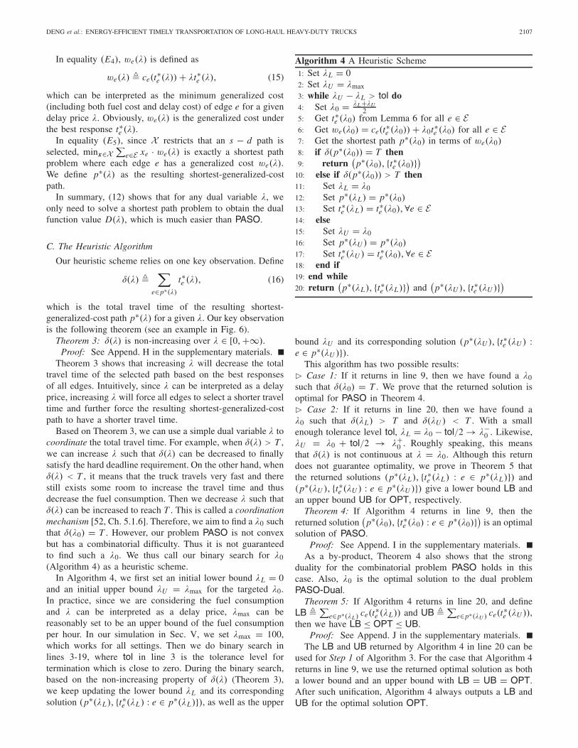
In Algorithm 4, we first set an initial lower bound λL = 0and an initial upper bound λU = λmax for the targeted λ0.In practice, since we are considering the fuel consumptionand λ can be interpreted as a delay price, λmax can bereasonably set to be an upper bound of the fuel consumptionper hour. In our simulation in Sec. V, we set λmax = 100,which works for all settings. Then we do binary search inlines 3-19, where tol in line 3 is the tolerance level fortermination which is close to zero. During the binary search,based on the non-increasing property of δ(λ) (Theorem 3),we keep updating the lower bound λL and its correspondingsolution (p∗(λL), {t∗e (λL ) : e ∈ p∗(λL)}), as well as the upper

Algorithm 4 A Heuristic Scheme1: Set λL = 02: Set λU = λmax3: while λU − λL > tol do4: Set λ0 = λL+λU

25: Get t∗e (λ0) from Lemma 6 for all e ∈ E6: Get we(λ0) = ce(t∗e (λ0)) + λ0t∗e (λ0) for all e ∈ E7: Get the shortest path p∗(λ0) in terms of we(λ0)8: if δ(p∗(λ0)) = T then9: return

(p∗(λ0), {t∗e (λ0)}

)10: else if δ(p∗(λ0)) > T then11: Set λL = λ012: Set p∗(λL) = p∗(λ0)13: Set t∗e (λL) = t∗e (λ0),∀e ∈ E14: else15: Set λU = λ016: Set p∗(λU ) = p∗(λ0)17: Set t∗e (λU ) = t∗e (λ0),∀e ∈ E18: end if19: end while20: return

(p∗(λL), {t∗e (λL)}) and

(p∗(λU ), {t∗e (λU )})

bound λU and its corresponding solution (p∗(λU ), {t∗e (λU ) :e ∈ p∗(λU )}).

This algorithm has two possible results:� Case 1: If it returns in line 9, then we have found a λ0such that δ(λ0) = T . We prove that the returned solution isoptimal for PASO in Theorem 4.� Case 2: If it returns in line 20, then we have found aλ0 such that δ(λL) > T and δ(λU ) < T . With a smallenough tolerance level tol, λL = λ0 − tol/2 → λ−

0 . Likewise,λU = λ0 + tol/2 → λ+

0 . Roughly speaking, this meansthat δ(λ) is not continuous at λ = λ0. Although this returndoes not guarantee optimality, we prove in Theorem 5 thatthe returned solutions (p∗(λL), {t∗e (λL) : e ∈ p∗(λL)}) and(p∗(λU ), {t∗e (λU ) : e ∈ p∗(λU )}) give a lower bound LB andan upper bound UB for OPT, respectively.

Theorem 4: If Algorithm 4 returns in line 9, then thereturned solution

(p∗(λ0), {t∗e (λ0) : e ∈ p∗(λ0)}

)is an optimal

solution of PASO.Proof: See Append. I in the supplementary materials.

As a by-product, Theorem 4 also shows that the strongduality for the combinatorial problem PASO holds in thiscase. Also, λ0 is the optimal solution to the dual problemPASO-Dual.

Theorem 5: If Algorithm 4 returns in line 20, and defineLB �

∑e∈p∗(λL ) ce(t∗e (λL)) and UB �

∑e∈p∗(λU ) ce(t∗e (λU )),

then we have LB ≤ OPT ≤ UB.Proof: See Append. J in the supplementary materials.

The LB and UB returned by Algorithm 4 in line 20 can beused for Step 1 of Algorithm 3. For the case that Algorithm 4returns in line 9, we use the returned optimal solution as botha lower bound and an upper bound with LB = UB = OPT.After such unification, Algorithm 4 always outputs a LB andUB for the optimal solution OPT.


1) Time Complexity: In line 7 in Algorithm 4, we useDijkstra’s shortest-path algorithm with a min-priority queue,which is the fastest known algorithm for the single-sourcesingle-destination shortest path problem with time complexityO(m + n log n) [53]. Thus, in the while loop, each itera-tion requires O(m log ξ + m + n log n) time. And since thetotal number of iterations is O(log λmax

tol ), Algorithm 4 hascomplexity O(m log ξ + m + n log n) log λmax

tol ), much fasterthan the FPTAS (Algorithm 3). We summarize the complexityresult in the following theorem.

Theorem 6: The time complexity of Algorithm 4 isO((m log ξ + m + n log n) log λmax

tol ).Remark: A similar dual-based heuristical approach for RSP

is proposed in [26]. However, as mentioned in Sec. III, differ-ent from RSP, our problem PASO has an extra design spaceof speed optimization. Therefore, theoretically our contributionin this section is to generalize the dual-based heuristical designfrom RSP [26] to PASO.

V. PERFORMANCE EVALUATION

In this section, we use real-world data to evaluatethe performance of our algorithms. Our objectives arethree-fold: (i) collect realistic dataset and model the fuel-rate-speed function, (ii) evaluate and compare the performance ofour FPTAS and heuristic, (iii) compare our algorithms withbaseline algorithms, including both shortest path algorithm andfastest path algorithm adapted from common practice, and (iv)investigate the energy-deadline tradeoff of long-haul heavy-duty trucks by evaluating how much fuel can be saved byincreasing the hard deadline.

A. Dataset

1) Transportation Network: We construct the U.S. NationalHighway Systems (NHS) from the dataset of ClinchedHighway Mapping (CHM) Project [54]. The whole high-way network graph file is specified in [55], which consistsof 84504 nodes (waypoints) and 89119 (one-direction) edges.

2) Elevation: In this paper, we consider the grade/slopeeffect when modeling the road-dependent fuel-rate-speed func-tion. To obtain the road grades, we use the Elevation PointQuery Service [56] provided by the U.S. Geological Sur-vey (USGS) to query elevations of all nodes in the NHS graph.

3) Speed Limits: We use the historical average speed asthe maximum speed Rub

e for each road e. HERE map [57]has put speed detectors over many countries including U.S.,and it provides APIs to query location-based real-time speedinformation. We collect the real-time speed information fromHERE map [57] for two weeks and use the average as Rub

efor each road e in the NHS graph5. For the minimum speedlimit Rlb

e , we manually set it to be Rlbe = min{30, Rub

e }.4) Fuel Consumption Data: It is hard for us to get suitable

real-world fuel consumption data. In this paper, we insteadleverage the widely-used ADVISOR simulator [58] to collectfuel consumption data (see Sec. V-B).

5Due to the truck’s gradeability, it may not achieve the average speed andthus later we also update Rub

e based on the maximum speed that the truckcan achieve at road e’s grade.

TABLE III

TRUCK PARAMETERS (KENWORTH T800)

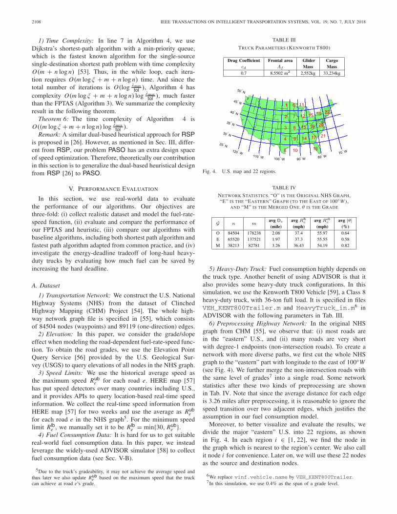
Fig. 4. U.S. map and 22 regions.

TABLE IV

NETWORK STATISTICS. “O” IS THE ORIGINAL NHS GRAPH,“E” IS THE “EASTERN” GRAPH (TO THE EAST OF 100◦W ),

AND “M” IS THE MERGED ONE. θ IS THE GRADE

5) Heavy-Duty Truck: Fuel consumption highly depends onthe truck type. Another benefit of using ADVISOR is that italso provides some heavy-duty truck configurations. In thissimulation, we use the Kenworth T800 Vehicle [59], a Class 8heavy-duty truck, with 36-ton full load. It is specified in filesVEH_KENT800Trailer.m and HeavyTruck_in.m6 inADVISOR with the following parameters in Tab. III.

6) Preprocessing Highway Network: In the original NHSgraph from CHM [55], we observe that: (i) most roads arein the “eastern” U.S., and (ii) many roads are very shortwith degree-1 endpoints (non-intersection roads). To create anetwork with more diverse paths, we first cut the whole NHSgraph to the “eastern” part with longitude to the east of 100◦W(see Fig. 4). We further merge the non-intersection roads withthe same level of grades7 into a single road. Some networkstatistics after these two kinds of preprocessing are shownin Tab. IV. Note that since the average distance for each edgeis 3.26 miles after preprocessing, it is reasonable to ignore thespeed transition over two adjacent edges, which justifies theassumption in our fuel consumption model.

Moreover, to better visualize and evaluate the results, wedivide the major “eastern” U.S. into 22 regions, as shownin Fig. 4. In each region i ∈ [1, 22], we find the node inthe graph which is nearest to the region’s center. We also callit node i for convenience. Later on, we will use these 22 nodesas the source and destination nodes.

6We replace vinf.vehicle.name by VEH_KENT800Trailer.7In this simulation, we use 0.4% as the span of a grade level.


TABLE V

FITTING PARAMETERS. FOR THE CONVEX REGION, ≤ x IS THE INTERVAL[0, x] AND ≥ x IS THE INTERVAL [x,∞)

B. Model Fuel-Rate-Speed Function

We model the fuel-rate-speed function as

fe(x) = aex3 + bex2 + cex + de,∀e ∈ E (17)

Here x is the speed (unit: mph) and fe(x) is the fuel rateconsumption (unit: gph (gallons per hour)). Although ourmodel (17) can capture any road-dependent features/factors,e.g., grade, rolling resistance, and air density, etc., we onlyconsider the road grade θ in this simulation, which is the majorfactor for truck fuel consumption [43].

To learn the parameters ae, be, ce and de in (17) interms of functions of θ , we use ADVISOR by invok-ing function adv_no_gui(action,input) where wespecify action=drive_cycle to run a driving cycletest [60, Ch. 2.3]. As mentioned in Sec. V-A, we choosethe default vehicle file HeavyTruck_in where we usevehicle type VEH_KENT800, which specifies Kenworth T800in Tab. III. For our purpose, we generate a driving cyclefile where we use a constant speed (say x (mph)) profileover a total of 4 hours and a constant grade (say θ ) overthe whole speed profile. Then after running ADVISOR, wecan get the total fuel consumption (say w (gallons)) over a4-hour driving time with speed x over a grade-θ road. Sincealmost all the time the truck runs with constant speed x , wecan get the corresponding fuel-rate consumption as w/4 (gph).By enumerating x from 10 mph to 70 mph with a stepof 0.2 mph, and enumerating θ from -10.0% to 10.0% with astep of 0.1%, we collect many (x, θ,w/4) data points.

For each grade θ from −10.0% to 10.0% with a stepof 0.1%, we use all (x, w/4) points to fit the model (17)by invoking MATLAB’s fit function. We sample severalgrade points in Tab. V, where we also put the strictly convexregion for the fitted fuel-rate-speed function fe(x). As we cansee, all fuel-rate-speed functions fe(·) are strictly convex inreasonable speed limit regions. For example, when grade is 0(a flat road), fe(·) is strictly convex if the speed is larger than14.22 mph, which holds generally in reality. This justifies ourassumption that the fuel-rate-speed function is polynomial andstrictly convex over the speed limit region.

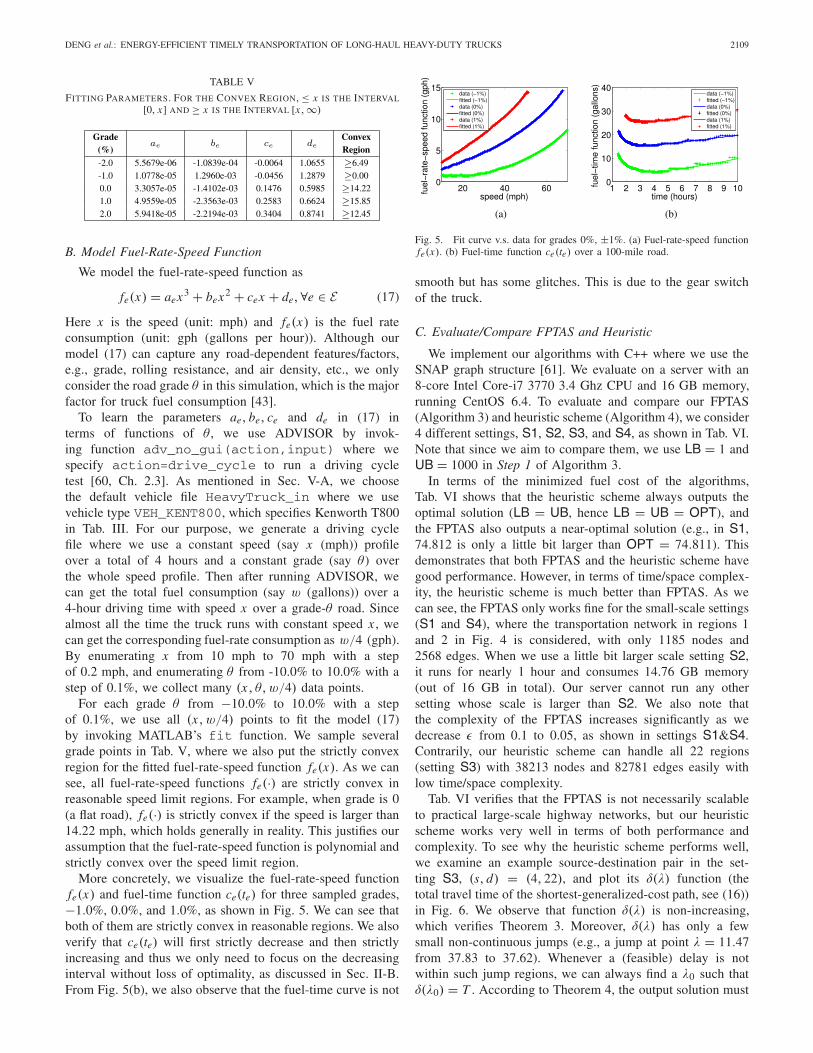
More concretely, we visualize the fuel-rate-speed functionfe(x) and fuel-time function ce(te) for three sampled grades,−1.0%, 0.0%, and 1.0%, as shown in Fig. 5. We can see thatboth of them are strictly convex in reasonable regions. We alsoverify that ce(te) will first strictly decrease and then strictlyincreasing and thus we only need to focus on the decreasinginterval without loss of optimality, as discussed in Sec. II-B.From Fig. 5(b), we also observe that the fuel-time curve is not

Fig. 5. Fit curve v.s. data for grades 0%, ±1%. (a) Fuel-rate-speed functionfe(x). (b) Fuel-time function ce(te) over a 100-mile road.

smooth but has some glitches. This is due to the gear switchof the truck.

C. Evaluate/Compare FPTAS and Heuristic

We implement our algorithms with C++ where we use theSNAP graph structure [61]. We evaluate on a server with an8-core Intel Core-i7 3770 3.4 Ghz CPU and 16 GB memory,running CentOS 6.4. To evaluate and compare our FPTAS(Algorithm 3) and heuristic scheme (Algorithm 4), we consider4 different settings, S1, S2, S3, and S4, as shown in Tab. VI.Note that since we aim to compare them, we use LB = 1 andUB = 1000 in Step 1 of Algorithm 3.

In terms of the minimized fuel cost of the algorithms,Tab. VI shows that the heuristic scheme always outputs theoptimal solution (LB = UB, hence LB = UB = OPT), andthe FPTAS also outputs a near-optimal solution (e.g., in S1,74.812 is only a little bit larger than OPT = 74.811). Thisdemonstrates that both FPTAS and the heuristic scheme havegood performance. However, in terms of time/space complex-ity, the heuristic scheme is much better than FPTAS. As wecan see, the FPTAS only works fine for the small-scale settings(S1 and S4), where the transportation network in regions 1and 2 in Fig. 4 is considered, with only 1185 nodes and2568 edges. When we use a little bit larger scale setting S2,it runs for nearly 1 hour and consumes 14.76 GB memory(out of 16 GB in total). Our server cannot run any othersetting whose scale is larger than S2. We also note thatthe complexity of the FPTAS increases significantly as wedecrease ε from 0.1 to 0.05, as shown in settings S1&S4.Contrarily, our heuristic scheme can handle all 22 regions(setting S3) with 38213 nodes and 82781 edges easily withlow time/space complexity.

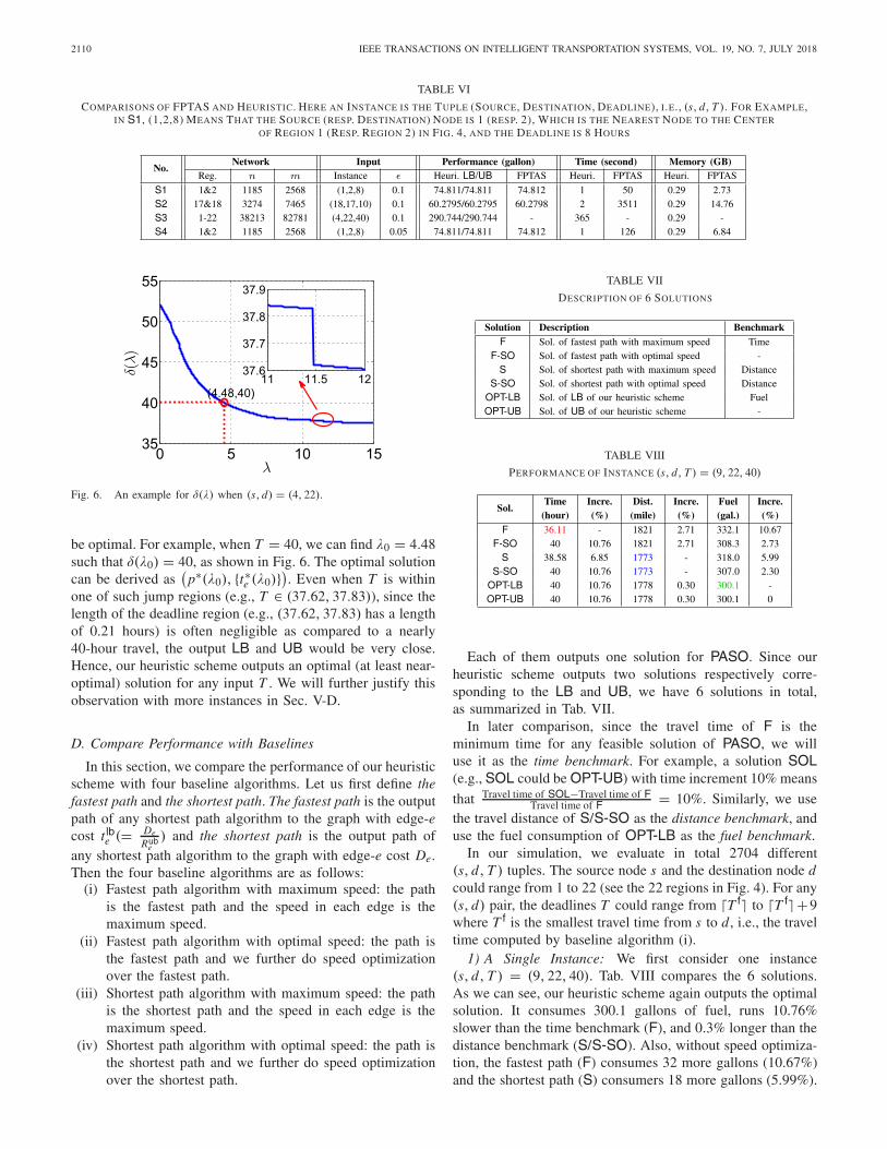
Tab. VI verifies that the FPTAS is not necessarily scalableto practical large-scale highway networks, but our heuristicscheme works very well in terms of both performance andcomplexity. To see why the heuristic scheme performs well,we examine an example source-destination pair in the set-ting S3, (s, d) = (4, 22), and plot its δ(λ) function (thetotal travel time of the shortest-generalized-cost path, see (16))in Fig. 6. We observe that function δ(λ) is non-increasing,which verifies Theorem 3. Moreover, δ(λ) has only a fewsmall non-continuous jumps (e.g., a jump at point λ = 11.47from 37.83 to 37.62). Whenever a (feasible) delay is notwithin such jump regions, we can always find a λ0 such thatδ(λ0) = T . According to Theorem 4, the output solution must


TABLE VI

COMPARISONS OF FPTAS AND HEURISTIC. HERE AN INSTANCE IS THE TUPLE (SOURCE, DESTINATION, DEADLINE), I.E., (s, d, T ). FOR EXAMPLE,IN S1, (1,2,8) MEANS THAT THE SOURCE (RESP. DESTINATION) NODE IS 1 (RESP. 2), WHICH IS THE NEAREST NODE TO THE CENTER

OF REGION 1 (RESP. REGION 2) IN FIG. 4, AND THE DEADLINE IS 8 HOURS

Fig. 6. An example for δ(λ) when (s, d) = (4, 22).

be optimal. For example, when T = 40, we can find λ0 = 4.48such that δ(λ0) = 40, as shown in Fig. 6. The optimal solutioncan be derived as

(p∗(λ0), {t∗e (λ0)}

). Even when T is within

one of such jump regions (e.g., T ∈ (37.62, 37.83)), since thelength of the deadline region (e.g., (37.62, 37.83) has a lengthof 0.21 hours) is often negligible as compared to a nearly40-hour travel, the output LB and UB would be very close.Hence, our heuristic scheme outputs an optimal (at least near-optimal) solution for any input T . We will further justify thisobservation with more instances in Sec. V-D.

D. Compare Performance with Baselines

In this section, we compare the performance of our heuristicscheme with four baseline algorithms. Let us first define thefastest path and the shortest path. The fastest path is the outputpath of any shortest path algorithm to the graph with edge-ecost t lb

e (= DeRub

e) and the shortest path is the output path of

any shortest path algorithm to the graph with edge-e cost De.Then the four baseline algorithms are as follows:

(i) Fastest path algorithm with maximum speed: the pathis the fastest path and the speed in each edge is themaximum speed.

(ii) Fastest path algorithm with optimal speed: the path isthe fastest path and we further do speed optimizationover the fastest path.

(iii) Shortest path algorithm with maximum speed: the pathis the shortest path and the speed in each edge is themaximum speed.

(iv) Shortest path algorithm with optimal speed: the path isthe shortest path and we further do speed optimizationover the shortest path.

TABLE VII

DESCRIPTION OF 6 SOLUTIONS

TABLE VIII

PERFORMANCE OF INSTANCE (s, d, T ) = (9, 22, 40)

Each of them outputs one solution for PASO. Since ourheuristic scheme outputs two solutions respectively corre-sponding to the LB and UB, we have 6 solutions in total,as summarized in Tab. VII.

In later comparison, since the travel time of F is theminimum time for any feasible solution of PASO, we willuse it as the time benchmark. For example, a solution SOL(e.g., SOL could be OPT-UB) with time increment 10% means

that Travel time of SOL−Travel time of FTravel time of F = 10%. Similarly, we use

the travel distance of S/S-SO as the distance benchmark, anduse the fuel consumption of OPT-LB as the fuel benchmark.

In our simulation, we evaluate in total 2704 different(s, d, T ) tuples. The source node s and the destination node dcould range from 1 to 22 (see the 22 regions in Fig. 4). For any(s, d) pair, the deadlines T could range from �T f� to �T f�+9where T f is the smallest travel time from s to d , i.e., the traveltime computed by baseline algorithm (i).

1) A Single Instance: We first consider one instance(s, d, T ) = (9, 22, 40). Tab. VIII compares the 6 solutions.As we can see, our heuristic scheme again outputs the optimalsolution. It consumes 300.1 gallons of fuel, runs 10.76%slower than the time benchmark (F), and 0.3% longer than thedistance benchmark (S/S-SO). Also, without speed optimiza-tion, the fastest path (F) consumes 32 more gallons (10.67%)and the shortest path (S) consumers 18 more gallons (5.99%).


Fig. 7. The delay effect when (s, d) = (9, 22).

TABLE IX

AVERAGE PERFORMANCE OF ALL 2704 INSTANCES

But with speed optimization, both fastest path and shortestpath have near-optimal performance.

For (s, d) = (9, 22), we also evaluate the effect of inputdeadline T as shown in Fig. 7. Considering speed optimization,when the input deadline T ∈ [36.11, 38.58), the shortestpath is infeasible, which shows that fastest path outper-forms shortest path. The shortest path becomes feasible whenT ≥ 38.58, and it outperforms the fastest path whenT > 39. This figure thus shows that the shortest pathbecomes better and better as the deadline constraint increases.Intuitively, when the hard deadline constraint can be satis-fied, the travel distance would be critical for the total fuelconsumption.

The OPT-UB curve in Fig. 7 is the energy-deadline tradeoffof (s, d) = (9, 22). We see that increasing deadline can savefuel consumption, and the saving has a “diminishing return”property. For example, the truck can save 6.6 gallons of fuelif it increases its deadline from 37 to 38 hours, but the savingreduces to 1.46 gallons if its deadline is relaxed from 45 to46 hours. A more comprehensive study on energy-deadlinetradeoff is shown in Sec. V-E.

2) All Instances: Similar to Tab. VIII, we can get the time,distance, and fuel of the 6 solutions for all source-sink pairs.We evaluate the average performance of all running instancesin terms of time/distance/fuel increments compared to thebenchmark numbers, as summarized in Tab. IX. Note that in4.84% of instances, shortest path is infeasible. Tab. IX only hasthe average performance over the instances where the shortestpath is feasible.

Tab. IX shows that on average OPT-UB only consumes0.02% of more fuels than the fuel benchmark (OPT-LB). This

Fig. 8. The energy-deadline tradeoff.

again shows that our heuristic scheme outputs a near-optimalsolution in all instances.

For the baseline algorithms, Tab. IX shows that the fastestpath (resp. shortest path) algorithm without speed optimizationconsumes 20.14% (resp. 16.40%) of more fuels than our solu-tion. In other words, our heuristic solution achieves 16.76%(resp. 14.09%) fuel consumption reduction, as compared tothe fastest path (resp. shortest path) algorithm. Our heuristicsolution also improves the 36-ton-truck’s fuel economy from5.05 for the fastest path and 5.13 for the shortest path to 5.96.Considering its significant portion of energy consumption, oursolution can indeed save much fuel cost for the long-haulheavy-duty trucks.

When we allow speed optimization for the fastest pathand the shortest path, we find that on average both of themare close to the optimal solution. More specifically, F-SOconsumes 2.00% of more fuels and S-SO only consumes0.31% of more fuels than OPT-LB. This apparently sug-gests that in the U.S., it is good enough to first choosethe shortest or fastest path and then do speed optimization.However, in our simulation, the shortest path is infeasibleamong 4.84% of all instances, and the fastest path withspeed optimization can consume 21.32% of more fuels in theworst instance. As opposed to them, our PASO solution isrobust in the sense that it always output a solution that isboth feasible and near-optimal. We also leave it as a futurework to understand under which conditions the fastest/shortestpath with speed optimization is close to the optimalsolution.

E. Energy-Deadline Tradeoff

In this subsection, we evaluate all (s, d) pairs where sand d range from 1 to 22. For each (s, d) pair, we first getthe smallest travel time T f, i.e., the travel time computed bybaseline algorithm (i) in Sec. V-D, and get the correspondingfuel consumption C f. Now we increase the deadline by x% andevaluate the fuel consumption C(x%) when T = (1 + x%)T f,and get the fuel consumption reduction C f−C(x%)

C f . By changingthe percentage of delay increase, i.e., x , we get different per-centages of fuel consumption reduction. The energy-deadlinetradeoff performance among all (s, d) pairs is shown inFig. 8.


As we can see, the fuel consumption reduction has a“diminishing return” property. As compared to the fastesttravel time, if we increase the hard deadline by 10%, we canreduce the fuel consumption by about 10% on average. Ifwe increase the hard deadline by 50%, we can reduce thefuel consumption by about 20% on average. If we furtherincrease the hard deadline after 70%, there is little extrabenefit. This is because the optimal running speed over mostedges becomes the minimum speed and there is little room todo further speed optimization if we increase the deadline morethan 70%.

VI. CONCLUSION AND FUTURE WORK

Provisioning both energy-efficient and timely delivery is ofgreat importance for logistic operators. This paper presentsa first step to study the energy-efficient timely transporta-tion problem with an emphasis for long-haul heavy-dutytrucks. We propose two algorithms: the first one is anFPTAS and the second one is a heuristic with lower com-plexity and near-optimal empirical performance. Our real-world data-driven simulations show that our solution guar-antees timely delivery and can save up to 17% of fuelconsumption as compared to a fastest/shortest path algorithmadapted from common practice. An interesting and impor-tant future direction is to generalize our results beyond thehighway setting to cover more sophisticated local drivingscenarios.

REFERENCES

[1] L. Deng, M. H. Hajiesmaili, M. Chen, and H. Zeng, “Energy-efficienttimely transportation of long-haul heavy-duty trucks,” in Proc. ACMe-Energy, 2016, Art. no. 10,

[2] (2014). Improving the Fuel Efficiency of American Trucks. [Online].Available: https://www.whitehouse.gov/the-press-office/2014/02/18/fact-sheet-opportunity-all-improving-fuel-efficiency-american-trucks-bol

[3] S. C. Davis, S. W. Diegel, and R. G. Boundy, Transportation EnergyData Book, 34th ed. Oak Ridge, TN, USA: U.S. Department of Energy,2015.

[4] Transportation Overview. Accessed: Sep. 13, 2017. [Online]. Available:http://www.c2es.org/energy/use/transportation

[5] W. F. Torrey and D. Murray, “An analysis of the operational costs oftrucking: A 2015 update,” Amer. Transp. Res. Inst., Arlington, VA, USA,Tech. Rep. 09-2015, 2015.

[6] W. Harrington and A. Krupnick, “Improving fuel economy in heavy-duty vehicles resources for the future DP,” Resour. Future, Washington,DC, USA, Tech. Rep. RFF-DP-12-02, 2012.

[7] Z. Mohamed-Kassim and A. Filippone, “Fuel savings on a heavy vehiclevia aerodynamic drag reduction,” Trans. Res. D, Transp. Environ.,vol. 15, no. 5, pp. 275–284, 2010.

[8] (2015). Supertruck Team Achieves 115% Freight EfficiencyImprovement in Class 8 Long-Haul Truck. [Online]. Available:http://energy.gov/eere/vehicles/articles/supertruck-team-achieves-115-freight-efficiency-improvement-class-8-long-haul

[9] U.S. Govt. Publish. Office, Laurel, MD, USA. KeepingYour Vehicle in Shape. [Online]. Available: https://www.fueleconomy.gov/feg/maintain.jsp

[10] F. Stodolsky, L. Gaines, and A. Vyas, “Analysis of technol-ogy options to reduce the fuel consumption of idling trucks,”Argonne Nat. Lab, Lemont, IL, USA, Tech. Rep. ANL/ESD-43,2000.

[11] A. A. Alam, A. Gattami, and K. H. Johansson, “Anexperimental study on the fuel reduction potential of heavyduty vehicle platooning,” in Proc. IEEE ITSC, Sep. 2010,pp. 306–311.

[12] J. Larson, K.-Y. Liang, and K. H. Johansson, “A distributed frameworkfor coordinated heavy-duty vehicle platooning,” IEEE Trans. Intell.Transp. Syst., vol. 16, no. 1, pp. 419–429, Feb. 2015.

[13] E. Demir, T. Bektas, and G. Laporte, “A review of recent research ongreen road freight transportation,” Eur. J. Oper. Res., vol. 237, no. 3,pp. 755–793, 2014.

[14] Y. Suzuki, “A new truck-routing approach for reducing fuel consumptionand pollutants emission,” Transp. Res. D, Transp. Environ., vol. 16, no. 1,pp. 73–77, 2011.

[15] M. Tunnell, “Estimating truck-related fuel consumption and emis-sions in maine: A comparative analysis for six-axle, 100,000 poundvehicle configuration,” in Proc. TRB 90th Annu. Meet., 2011,pp. 1–12.

[16] E. Hellström, M. Ivarsson, J. Åslund, and L. Nielsen, “Look-ahead control for heavy trucks to minimize trip time and fuelconsumption,” Control Eng. Pract., vol. 17, no. 2, pp. 245–254,2009.

[17] E. Hellström, J. Åslund, and L. Nielsen, “Design of an efficient algo-rithm for fuel-optimal look-ahead control,” Control Eng. Pract., vol. 18,no. 11, pp. 1318–1327, 2010.

[18] (2011). Smarter Trucking Saves Fuel Over the Long Haul. [Online].Available: http://news.nationalgeographic.com/news/energy/2011/09/110923-fuel-economy-for-trucks/

[19] Fuel Economy at Various Driving Speeds. Accessed: Sep. 13, 2017.[Online]. Available: http://www.afdc.energy.gov/data/10312

[20] W. Mallett, “Freight performance measurement: Travel time in freight-significant corridors,” U.S. Federal Highway Admin., Washington, DC,USA, Tech. Rep. FHWA-HOP-07-071, 2006.

[21] (2014). Transportation Logistics Enhances Your Business Efficiency.[Online]. Available: http://www.readytrucking.com/transportation-logistics-business-efficiency/

[22] B. H. Ashby, “Protecting perishable foods during transport bytruck,” U.S. Dept. Agricult., Washington, DC, USA, Tech. Rep. 669,2006.

[23] Place an Order With Guaranteed Delivery. Accessed: Sep. 13, 2017.[Online]. Available: https://www.amazon.com/gp/help/customer/display.html/ref=hp_left_v4_sib?ie=UTF8&nodeId=201117390

[24] R. Hassin, “Approximation schemes for the restricted shortest pathproblem,” Math. Oper. Res., vol. 17, no. 1, pp. 36–42, 1992.

[25] M. R. Garey and D. S. Johnson, Computers and Intractability; A Guideto the Theory of NP-Completeness. New York, NY, USA: Freeman,1990.

[26] A. Jüttner, B. Szviatovski, I. Mécs, and Z. Rajkó, “Lagrange relaxationbased method for the QoS routing problem,” in Proc. IEEE INFOCOM,Apr. 2001, pp. 859–886.

[27] M. W. Savelsbergh, “Local search in routing problems withtime windows,” Ann. Oper. Res., vol. 4, no. 1, pp. 285–305,1985.

[28] L. M. Gambardella, E. Taillard, and G. Agazzi, “MACS-VRPTW:A multiple ant colony system for vehicle routing problems with timewindows,” Dalle Molle Inst. Artif. Intell. Res., Manno, Switzerland,Tech. Rep. tr-idsia-06-99, 1999.

[29] J.-F. Cordeau, G. Laporte, and A. Mercier, “A unified tabu searchheuristic for vehicle routing problems with time windows,” J. Oper.Res. Soc., vol. 52, no. 8, pp. 928–936, 2001.

[30] K. C. Tan, L. H. Lee, Q. Zhu, and K. Ou, “Heuristic methods for vehiclerouting problem with time windows,” Artif. Intell. Eng., vol. 15, no. 3,pp. 281–295, 2001.

[31] J. Qian and R. Eglese, “Fuel emissions optimization in vehicle routingproblems with time-varying speeds,” Eur. J. Oper. Res., vol. 248, no. 3,pp. 840–848, 2016.

[32] I. Norstad, K. Fagerholt, and G. Laporte, “Tramp ship routing andscheduling with speed optimization,” Transp. Res. C, Emerg. Technol.,vol. 19, no. 5, pp. 853–865, 2011.

[33] P. Serafini, “Some considerations about computational complexity formulti objective combinatorial problems,” in Recent Advances and His-torical Development of Vector Optimization. Berlin, Germany: Springer,1987, pp. 222–232.

[34] G. Tsaggouris and C. Zaroliagis, “Multiobjective optimization: ImprovedFPTAS for shortest paths and non-linear objectives with appli-cations,” Theory Comput. Syst., vol. 45, no. 1, pp. 162–186,2009.

[35] T. Breugem, T. Dollevoet, and W. van den Heuvel, “Analysis of FPTASesfor the multi-objective shortest path problem,” Comput. Oper. Res.,vol. 78, pp. 44–58, Feb. 2017.

[36] K. Ghoseiri and B. Nadjari, “An ant colony optimization algorithm forthe bi-objective shortest path problem,” Appl. Soft Comput., vol. 10,no. 4, pp. 1237–1246, 2010.


[37] G. Scora, K. Boriboonsomsin, and M. Barth, “Value of eco-friendlyroute choice for heavy-duty trucks,” Res. Transp. Econ., vol. 52,pp. 3–14, Oct. 2015.

[38] (2013). Energy Consumption Estimates by End-Use Sector,Ranked by State. [Online]. Available: http://www.eia.gov/state/seds/data.cfm?incfile=/state/seds/sep_sum/html/rank_use.html&sid=US

[39] N. T. Moungla, L. Létocart, and A. Nagih, “Solutions diversification ina column generation algorithm,” Algorithmic Oper. Res., vol. 5, no. 2,pp. 86–95, 2010.

[40] F. Vanderbeck, “Computational study of a column generation algorithmfor bin packing and cutting stock problems,” Math. Programm., vol. 86,no. 3, pp. 565–594, 1999.

[41] N. L. J. Ulder, E. H. L. Aarts, H.-J. Bandelt, P. J. M. van Laarhoven,and E. Pesch, “Genetic local search algorithms for the traveling salesmanproblem,” in Parallel Problem Solving from Nature. Berlin, Germany:Springer, 1991, pp. 109–116.

[42] E. Demir, T. Bektas, and G. Laporte, “A comparative analysis ofseveral vehicle emission models for road freight transportation,” Transp.Res. D, Transp. Environ., vol. 16, no. 5, pp. 347–357, Jul. 2011.

[43] K. Ahn, “Microscopic fuel consumption and emission modeling,”M.S. thesis, Dept. Civil Environ. Eng., Virginia Polytech. Inst. StateUniv., Blacksburg, VA, USA, 1998.

[44] D. J. Chang and E. K. Morlok, “Vehicle speed profiles to minimize workand fuel consumption,” J. Transp. Eng., vol. 131, no. 3, pp. 173–182,2005.

[45] A. Fröberg, E. Hellström, and L. Nielsen, “Explicit fuel optimalspeed profiles for heavy trucks on a set of topographic road profiles,”SAE Int., Warrendale, PA, USA, Tech. Rep. 2006-01-1071, 2006.

[46] G. Yang, H. Xu, Z. Wang, and Z. Tian, “Truck acceleration behaviorstudy and acceleration lane length recommendations for metered on-ramps,” Int. J. Transp. Sci. Technol., vol. 5, no. 2, pp. 93–102, 2016.

[47] S. Ardekani, E. Hauer, and B. Jamei, “Traffic impact models chapter7 in traffic flow theory,” Oak Ridge Nat. Lab., Oak Ridge, TN, USA,Tech. Rep., 1992.

[48] F. An and M. Ross, “Model of fuel economy with applications todriving cycles and traffic management,” Transp. Res. Record, no. 1416,pp. 105–114, 1993.

[49] E. K. Nam and R. Giannelli, “Fuel consumption modeling of conven-tional and advanced technology vehicles in the physical emission rateestimator (PERE),” U.S. Environ. Protect. Agency, Washington, DC,USA, Tech. Rep. EPA420-P-05-001, 2005.

[50] I. M. Berry, “The effects of driving style and vehicle performance onthe real-world fuel consumption of U.S. light-duty vehicles,” M.S. thesis,Dept. Mech. Eng., Massachusetts Inst. Technol., Cambridge, MA, USA,2010.

[51] D. H. Lorenz and D. Raz, “A simple efficient approximation scheme forthe restricted shortest path problem,” Oper. Res. Lett., vol. 28, no. 5,pp. 213–219, 2001.

[52] D. P. Bertsekas, Nonlinear Programming. Belmont, MA, USA:Athena Scientific, 1999.

[53] Dijkstra’s Algorithm. [Online]. Available: https://en.wikipedia.org/wiki/Dijkstra%27s_algorithm

[54] J. D. Teresco. The Clinched Highway Mapping (CHM) Project.Accessed: Sep. 13, 2017. [Online]. Available: http://cmap.m-plex.com/

[55] CHM U.S. National Highway Systems. Accessed: Sep. 13, 2017.[Online]. Available: http://courses.teresco.org/chm/graphs/usa-national.gra

[56] USGS Elevation Point Query Service. Accessed: Sep. 13, 2017. [Online].Available: http://nationalmap.gov/epqs/

[57] Traffic Flow Using Corridor in HERE Maps. Accessed:Sep. 13, 2017. [Online]. Available: https://developer.here.com/api-explorer/rest/traffic/flow-using-corridor

[58] T. Markel et al., “ADVISOR: A systems analysis tool for advancedvehicle modeling,” J. Power Sour., vol. 110, no. 2, pp. 255–266, 2002.

[59] Kenworth T800 Vehicle. Accessed: Sep. 13, 2017. [Online]. Available:http://www.kenworth.com/trucks/t800

[60] ADVISOR Documentation. Accessed: Sep. 13, 2017. [Online]. Available:http://adv-vehicle-sim.sourceforge.net/advisor_doc.html

[61] J. Leskovec and R. Sosic. (2014). SNAP: A General Purpose NetworkAnalysis and Graph Mining Library in C++. [Online]. Available:http://snap.stanford.edu/snap

[62] F. Mannering, W. Kilareski, and S. Washburn, Principles of HighwayEngineering and Traffic Analysis. Hoboken, NJ, USA: Wiley, 2007.

[63] A. Jeffrey and D. Zwillinger, Table of Integrals, Series, and Products,7th ed. San Diego, CA, USA: Academic, 2007.

Lei Deng received the B.Eng. degree from theDepartment of Electronics Engineering, ShanghaiJiao Tong University, Shanghai, China, in 2012,and the Ph.D. degree from the Department ofInformation Engineering, The Chinese Universityof Hong Kong, Hong Kong, in 2017. In 2015,he was a Visiting Scholar with the School of Elec-trical and Computer Engineering, Purdue University,West Lafayette, IN, USA. His research interestsare timely network communications, energy-efficienttimely transportation, and spectral-energy efficiencyin wireless networks.

Mohammad H. Hajiesmaili received the B.Sc.degree in computer engineering from the Depart-ment of Computer Engineering, Sharif University ofTechnology, Iran, in 2007, and the M.Sc. and Ph.D.degrees in computer engineering from the Electricaland Computer Engineering Department, Universityof Tehran, Iran, in 2009 and 2014, respectively.He was a Post-Doctoral Fellow with the Departmentof Information Engineering, The Chinese Universityof Hong Kong, from 2014 to 2016. He is currently aPost-Doctoral Fellow with the Department of Elec-

trical and Computer Engineering, Johns Hopkins University. His researchinterests include optimization, algorithm, and mechanism design in commu-nication, energy, and transportation networks.

Minghua Chen (S’04–M’06–SM’13) received theB.Eng. and M.S. degrees from the Departmentof Electronic Engineering, Tsinghua University,in 1999 and 2001, respectively, and the Ph.D.degree from the Department of Electrical Engineer-ing and Computer Sciences, University of Californiaat Berkeley, in 2006. He spent one year visitingMicrosoft Research Redmond as a Post-DoctoralResearcher. He joined the Department of Infor-mation Engineering, The Chinese University ofHong Kong, in 2007, where he is currently an Asso-

ciate Professor. He is also an Adjunct Associate Professor with the Instituteof Interdisciplinary Information Sciences, Tsinghua University. His currentresearch interests include energy systems (e.g., smart power grids and energy-efficient datacenters), intelligent transportation system, wireless networking,multimedia networking, online competitive optimization, distributed optimiza-tion, and delay-constrained network information flow. He received the Eli JuryAward from UC Berkeley in 2007 (presented to a graduate student or recentalumnus for outstanding achievement in the area of systems, communications,control, or signal processing) and The Chinese University of Hong KongYoung Researcher Award in 2013. He also received several best paper awards,including the IEEE ICME Best Paper Award in 2009, the IEEE Transactionson Multimedia Prize Paper Award in 2009, and the ACM Multimedia BestPaper Award in 2012. He receives the ACM Recognition of Service Awardin 2017 for service contribution to the research community. He is currentlyan Associate Editor of the IEEE/ACM TRANSACTIONS ON NETWORKING.He serves as TPC Co-Chair of ACM e-Energy 2016 and the General Chairof ACM e-Energy 2017.

Haibo Zeng received the Ph.D. degree in elec-trical engineering and computer sciences from theUniversity of California at Berkeley. He was aSenior Researcher with General Motors Researchand Development until 2011, and an Assistant Pro-fessor with McGill University until 2014. He iscurrently an Assistant Professor with Virginia Tech,Blacksburg, VA, USA. His research interests aredesign methodology, analysis, and optimization forembedded systems, cyber-physical systems, andreal-time systems. He earned three best paper

citations in his research fields.

Energy-Efficient Timely Transportation of Long-Haul Heavy ...

Documents

Transcript of Energy-Efficient Timely Transportation of Long-Haul Heavy ...