Energy-Efficient Routing Algorithms in Wireless Sensor...

of 29

Energy-Efficient Routing Algorithms in Wireless Sensor Networks: e3D Diffusion vs. Clustering

ABSTRACT

One of the limitations of wireless sensor nodes is their inherent limited energy resource. Besides maximizing the

lifetime of the sensor node, it is preferable to distribute the energy dissipated throughout the wireless sensor network in

order to minimize maintenance and maximize overall system performance. Any communication protocol that involves

synchronization of peer nodes incurs some overhead for setting up the communication. We introduce a new algorithm,

e3D*, and compare it to two other algorithms, namely directed, and random clustering communication. We take into

account the setup costs and analyze the energy-efficiency and the useful lifetime of the system. In order to better

understand the characteristics of each algorithm and how well e3D really performs, we also compare e3D with its

optimum counterpart and an optimum clustering algorithm. The benefit of introducing these ideal algorithms is to show

the upper bound on performance at the cost of an astronomical prohibitive synchronization costs. We compare the

algorithms in terms of system lifetime, power dissipation distribution, cost of synchronization, and simplicity of the

algorithm. Our simulation results show that e3D performs only slightly worse than its optimal counterpart while having

much less overhead. Therefore, our contribution is a diffusion based routing protocol that prolongs the system lifetime,

evenly distributes the power dissipation throughout the network, and incurs minimal overhead for synchronizing

communication.

Keywords: e3D, wireless sensor networks, energy-efficient, routing algorithm, diffusion routing, clustering

1.0 INTRODUCTION

Over the last half a century, computers have exponentially increased in processing power and at the same time

decreased in both size and price. These rapid advancements led to a very fast market in which computers would

participate in more and more of our society’s daily activities. In recent years, one such revolution has been taking place,

Department of Computer Science Purdue University

West Lafayette, IN 47907, USA [email protected]

Ioan Raicu

CS590N Project Report Project Supervisor: Dr. Dongyan Xu

________________________________ * e3D is the acronym denoting the proposed energy-efficient Distributed Dynamic Diffusion routing algorithm.

of 29

where computers are becoming so small and so cheap, that single-purpose computers with embedded sensors are almost

practical from both economical and theoretical points of view. Wireless sensor networks are beginning to become a

reality, and therefore some of the long overlooked limitations have become an important area of research.

In this paper, we attempt to overcome limitations of the wireless sensor networks such as: limited energy resources,

varying energy consumption based on location, high cost of transmission, and limited processing capabilities. All of

these characteristics of wireless sensor networks are complete opposites of their wired network counterparts, in which

energy consumption is not an issue, transmission cost is relatively cheap, and the network nodes have plenty of

processing capabilities. It should be obvious that routing approaches that have worked so well in traditional networks

for over twenty years will not suffice for this new generation of networks.

Besides maximizing the lifetime of the sensor nodes, it is preferable to distribute the energy dissipated throughout the

wireless sensor network in order to minimize maintenance and maximize overall system performance [5,6,7]. Any

communication protocol that involves synchronization between peer nodes incurs some overhead of setting up the

communication. We attempt to calculate this overhead and to come to a conclusion whether the benefits of more

complex routing algorithms overshadow the extra control messages each node needs to communicate. Obviously, each

node could make the most informed decision regarding its communication options if they had complete knowledge of

the entire network topology and power levels of all the nodes in the network. This indeed proves to yield the best

performance if the synchronization messages are not taken into account. However, since all the nodes would always

have to know everything, it should be obvious that there will be many more synchronization messages than data

messages, and therefore ideal case algorithms are not feasible in a system where communication is very expensive. For

both the diffusion and clustering algorithms, we will analyze both realistic and optimum schemes in order to gain more

insight in the properties of both approaches.

The usual topology of wireless sensor networks involves having many network nodes dispersed throughout a specific

physical area. There is usually no specific architecture or hierarchy in place and therefore, the wireless sensor networks

are considered as ad hoc networks. That does not mean that a dynamic organization is not allowed, however it just

cannot be predefined in advance.

An ad hoc wireless sensor network is an autonomous system of sensor nodes in which all nodes act as routers connected

by wireless links. Although ad hoc networks usually imply that nodes are free to move randomly and organize

themselves arbitrarily, in this paper we considered only ad hoc networks with fixed node positions. On the other hand,

of 29

wireless links are not very reliable and nodes might stop operating at arbitrary points within the system’s life; therefore,

the routing protocol utilized must be able to handle arbitrary failure of nodes throughout the network. Such a network

may operate in a standalone fashion, or it may be connected to other networks, such as the larger Internet. This

architecture leads to the concept of peer-to-peer communication throughout the wireless sensor network for

communication between most of the network nodes, and client-server communication between some nodes and the base

station [2]. Eventually, the data retrieved by the sensors must be propagated back to a central location, where further

processing must be done in order to analyze the data and extract meaningful information from the large amounts of data.

Therefore, a base station(s) is usually elected in order to act as the gateway between the wireless network and IEEE

802.x networks [13], such as wired Ethernet, or perhaps 802.11 Wireless Ethernet [14]. Base stations are usually more

complex than mere network nodes since they must have dual purpose functionality: one to communicate with the

wireless network and the other to communicate with the wired network. It also usually has an unlimited power supply

and therefore, power consumption is not critical for the base station. With a large enough transmit power, and in

essence very large power consumption, each node could theoretically communicate with the base station; however due

to a limited power supply, spatial reuse of wireless bandwidth, and the nature of radio communication cost which is a

function of the distance transmitted squared, it is ideal to send information in several smaller distance wise steps rather

than one transmission over a long communication distance [3,4].

Some typical applications for wireless sensors include the collection of massive amounts of sensor data. Furthermore,

the sensors can extend mobile device functionality, such as providing input to mobile computer applications and

receiving commands from mobile computers. They can facilitate communication with the user’s environment, such as

beacons or sources of information throughout the physical space [10]. Some other typical examples are environmental

sensors, automotive sensors, highway monitoring sensors, and biomedical sensors.

In our simulation, we use a data collection problem in which the system is driven by rounds of communication, and

each sensor node has a packet to send to the distant base station. The diffusion algorithm is based on location, power

levels, and load on the node, and its goal is to distribute the power consumption throughout the network so that the

majority of the nodes consume their power supply at relatively the same rate regardless of physical location. This leads

to better maintainability of the system, such as replacing the batteries all at once rather than one by one, and maximizing

the overall system performance by allowing the network to function at 100% capacity throughout most of its lifetime

instead of having a steadily decreasing node population.

of 29

The rest of the paper is organized as follows. Section 2 covers background information and previous work completed in

the field, assumptions, algorithms, findings, and shortcomings. Section 3 covers our evaluation test-bed; we explain our

own realistic assumptions based on real world sensors, the sensors hardware on which we based our assumptions, and

the distribution of the sensor nodes. Section 4 covers the description and cost analysis of six routing algorithms: direct

communication, basic diffusion routing algorithm, e3D routing algorithm (diffusion based and our contribution), ideal

diffusion based routing algorithm, random clustering, and the ideal clustering routing algorithm. We finally conclude

with Section 5 in which we talk about the importance of our findings and future work.

2.0 BACKGROUND INFORMATION AND RELATED WORK

As we discussed in the previous Section, the major issues concerning wireless sensor networks are power management,

longevity, functionality, sensor data fusion, robustness, and fault tolerance. Power management deals with extending

battery life and reducing power usage while longevity concerns the co-ordination of sensor activities and optimizations

in the communication protocol. The functionality deals with future targeted applications. Data fusion encompasses the

combining of sensor data, or perhaps data compression. Obviously, robustness and fault tolerance deals with failing

nodes and the erroneous characteristic of the wireless communication medium.

Some progress has been made toward overcoming some of these major issues. For example, LEACH (Low-Energy

Adap-tive Clustering Hierarchy) [8] and PEGASIS (Power-Efficient GAthering in Sensor Information Systems) [9]

have very similar goals compared to what we are proposing. Therefore, we ill discuss briefly some of their

assumptions, algorithms, findings, and shortcomings. It is also worthwhile to mention a routing algorithm, namely

directed diffusion [15], which has a similar name but is quite different than our proposed diffusion based algorithm.

2.1 Directed Diffusion

Directed diffusion is a paradigm for coordination of distributed sensing [15]. Although this is similar to our goals, it is

a data centric in that all communication is for named data. It is designed for query driven network communication and

in having dynamic multiple paths from any one node to another. It first finds a best path by diffusing a message into the

network and waiting for a message identifying the best path. Alternate paths are kept for robustness in case some nodes

along the way fail.

of 29

It should not be too difficult to realize how our approach differs. First of all, our goal is not to create a routing

algorithm that will find the best path from any node to any other node in the network. Furthermore, the directed

diffusion is based on a query driven architecture while our e3D approach is an event driven architecture in which

messages are generated at regular intervals and sent towards a central location. Therefore, we have narrowed the

definition of the problem to having a single base station to which all nodes in the network must find the best path. Since

our problem is more constrained, our suggested approach will produce much less overhead than in the more generalized

problem addressed in directed diffusion.

2.2 LEACH

In order to better understand the argument for both LEACH and PEGASIS, we will briefly discuss the definition of

clustering in the traditional sense. The definition of clustering according to [11] is:

“A cluster is an aggregation of points in the test space such that the distance between any two points in the

cluster is less than the distance between any point in the cluster and any point not in it.”

Although this definition is given from the field of Data Analysis and Pattern Recognition, it is the classical

representation for clustering and should be used based on its strictest definition whenever possible in order to utilize the

benefits of clustering approach.

As an overview, LEACH is a clustering-based protocol that utilizes randomized rotation of cluster heads to evenly

distribute the energy load among the sensors in the network. LEACH uses localized coordination to enable scalability

and robustness for dynamic networks, and incorporates data aggregation into the routing protocol to reduce the amount

of information that must be transmitted to the base station. The cluster heads are randomly chosen in order to

randomize the distribution of the energy consumption and load among the sensors, and therefore taking the first step

towards evenly distributing the energy consumption through the system’s lifetime. Each cluster head acts as a gateway

between the cluster members and the base station; the cluster head aggregates all the information received from its

members and then sends one message directly to the base station. Note that the one message size that is sent to the base

station is size independent from the number of messages the cluster head receives from its members.

LEACH utilized a 100 nodes network with randomly chosen fixed positions and a 50 by 50 meter area of distribution.

The cluster heads are randomly chosen and are only chosen for a specific duration of time. Each node transmits at a

fixed rate, and always has data to transmit; they utilize fixed size packets of 2000 bits each. Their power consumption

of 29

constants were: 50 nJ/bit for either transmitting or receiving electronics, and 100 pJ/bit/m2 for transmitting

amplification.

The positive point in randomized cluster heads is the fact that the nodes will randomly deplete their power supply, and

therefore they should randomly die throughout the network. Since the clustering implemented in LEACH is based on

randomness, its cost is much less and realistically feasible when compared to the traditional clustering definition.

Although LEACH’s clustering protocol seems promising, further evaluation is needed in analyzing the set up and

synchronization costs of maintaining the LEACH protocol.

One the other hand, the randomized cluster heads will make it very difficult to achieve optimal results. It should also be

obvious that since random numbers are utilized, the performance of the system will vary according to the random

number generation and will not be as predictable as a system that is based on information that will lead it to make the

best local decision possible. For LEACH to be a true clustering protocol as defined above, the cluster heads should be

chosen according to certain metrics, such as location, power levels, etc. Figuring out the clusters topology requires

global knowledge of every nodes position, which requires global synchronization. If the cluster heads would only have

to be chosen once, the cost of obtaining the global information might be plausible, however since the cluster heads

would deplete their energy supply much faster than the rest of the nodes, each node can only be a cluster head

temporarily, which implies that the clustering global synchronization would have to be done rather frequently.

The second drawback of LEACH is the assumption that 100% aggregation of data is a common characteristic of real

world systems. There are applications where this assumption is reasonable, however most applications rely on the

availability of more information to be finally received for evaluation and analysis. In LEACH, for each round, each

cluster head receives a packet of 2000 bits from x number of child nodes; it fuses all received packets together, 2000*x

bits, and sends one packet of 2000 bits to the base station that is supposed to represent the data contained in x number of

packets. It therefore assumes that a saving of a factor of x can be reasonably achieved. However, in practice, this

technique would lead to much missing data and most likely unsuitable for most applications.

2.3 PEGASIS

PEGASIS, a near optimal chain-based protocol, is an improvement over LEACH. In PEGASIS, group heads are chosen

randomly and each node communicates only with a close neighbor forming a chain leading to its cluster head. It is

essentially a multi-hop clustering approach to solving energy-efficiency problem addressed by this paper. The

of 29

randomization of the cluster heads will guarantee that the nodes will die in a random order throughout the network, thus

keeping the density throughout the network proportional.

PEGASIS assumes to have global knowledge of the network topology and therefore uses a greedy algorithm when

constructing a chain. It starts with the farthest node from the base station, which ensures that the nodes farthest away

from the base station have an accessible neighbor. With each dying node, the chain is reconstructed; the leader of each

round of communication will be at a random place selected in the chain. As the data moves from node to node in the

chain, it is fused together. Eventually the designated node in the chain will transmit the fused packet to the base station.

Notice that PEGASIS has the same aggregation schema, where each node sends a packet of 2000 bits, while each next

node in the chain only transmits a packet of 2000 bits, regardless where in the chain it is situated. It should be clear that

at every level in the chain, the data is aggregated from 2 packets of 2000 bits each into 1 packet of 2000 bits.

PEGASIS is an interesting approach, however there is the potential to achieve better performance for many applications

because of three reasons. The clustering is based on random cluster heads, 100% aggregation is not realistic for many

applications, and the chain described in PEGASIS is not an optimal routing mechanism in terms of the distance the data

needs to traverse. LEACH proposed that each child node directly send its data to the cluster head. PEGASIS improved

that by making each child node communicate over smaller hops by forming a chain, which by design should improve on

the power consumption since radio transmissions cost on the order of the distance transmitted squared. The chain is

obviously optimal for this type of approach, but other approaches such as diffusion could give better performance. In

forming the chain, nodes might send their data in various directions, even backwards, which may be counterproductive.

A possible solution to the above limitation would be to allow each node making the best decision for itself, namely a

greedy algorithm approach, which would result in a system that all nodes would be transmitting to the best neighbor in

each one’s respective opinion. There is a need for a mechanism to not allow loop formations, however it becomes a

trivial exercise once the solution is visualized in Section 4.2. Greedy algorithms can produce optimal results in many

problems and application. According to our findings, using the greedy algorithm for wireless sensor networks as a

routing decision mechanism seems to provide a near optimal routing mechanism for distributing the power dissipation

and prolonging the system lifetime. This is our proposed system called e3D and is described in detail in Section 4.3.

of 29

3.0 SIMULATION TEST-BED AND ASSUMPTIONS

In this Section, we describe the assumptions we based our findings on and the basis of the assumptions. In Section 3.1,

we briefly describe the wireless sensors “Rene RF motes” and their operating system, the TinyOS [12]. In Section 3.2,

we present the simulation constants we assumed in our simulations. In Section 3.3, we describe the random distribution

used to establish the positions of all the nodes.

3.1 Software/Hardware Architecture

Our simulation is based on real world wireless sensors, specifically the Rene RF motes designed at University of

California, Berkeley (UCB) [12]. We decided to base our work on these sensors purely because they offer a good

architecture to validate the findings of this paper. An important aspect of our research is that the details of power

consumption or the energy capacity of the battery supply for each wireless sensor is almost irrelevant since the results

between the various algorithms should remain relatively the same to each other.

A brief overview of the sensor hardware and software is described below. We used the RENE RF Mote which runs the

TinyOS, a very small footprint, event-driven operating system designed for computers with limited processing power

and battery life. A mote consists of a mote motherboard and an optional sensor board that plugs into the mote

motherboard and includes both a photo and temperature sensor can be used as well.

The RENE RF Motes utilize the ATMEL processor (90LS8535), which is an 8-bit Harvard architecture with 16-bit

addresses. It provides 32 8-bit general registers and runs at 4 MHz and requires a 3.0 volt power supply. The system is

very memory constrained: it has 8 KB of flash as the program memory, and 512 bytes of SRAM as the data memory.

Additionally, the processor integrates a set of timers and counters which can be configured to generate interrupts at

regular time intervals.

The radio consists of an RF Monolithic 916.50 MHz transceiver, antenna, and a collection of discrete components to

configure the physical layer characteristics, such as signal strength and sensitivity. It operates at speeds up to 19.2 Kbps,

115 Kbps using amplitude shift keying, but usually about 10 Kbps as raw data; the speeds are as low as they are because

of the bit-level processing, and the conservation of the most valuable resource – battery life. Control signals configure

the radio to operate in either transmit, receive, or power-off mode. The radio contains no buffering so each bit must be

serviced by the controller in real time.

of 29

The task scheduler is just a simple FIFO scheduler. The range of the motes communication is about 100 ft; the signal

strength can be controlled through a digital potentiometer from 0 ~ 50 kOhms. All the motes contend for a single

channel RF radio; they use carrier sense multiple access (CSMA) and have no collision detection mechanism. Channel

capacity is about 25 packets per second, so the wireless network can easily get congested if too many sensors are within

communication range of each other.

The sensors utilize a 3 volt power supply, as long as the voltage lies between about 2.8 volts and 3.6 volts. Our

experiments are based on using two Duracell AA 1.5V alkaline batteries @ 1850 mAh each, which produce about 15

Kilo Joules of energy. In the real world, we would expect a mote to have enough power to last about 4 days under

active (100% utilization) communication, and about 125 days under an idle state.

3.2 Simulation Constants

According to Table 1, we establish the constants that drive the simulation results. The following table will show a

detailed list of these constants and their explanations.

Name Description Value

float BW Link bandwidth between peer nodes 10 Kbit/s

float Interval 1 message every XXX seconds 10 second

int MsgByte Total size of the packet 50 bytes

float TxAmp Transmission amplification cost for radio transmitter as a function related to distance transmitted and bits processed

1.8 micro joule/bit/m2

float TxCost Transmission cost for running the radio circuitry per bits processed 2.51789 micro joule/bit

float RxCost Reception cost for running the radio circuitry per bit processed 2.02866 micro joule/bit

float IdleCost The cost for a mote to be in its idle state; it is a function related to time 1000 micro joule/second

float InitPowerJ The initial energy each mote is given; depends on the type of battery used. 15390 joule

int areaSize The length of the side of the area used for distributing the motes 100 meters

int netSize The number of nodes in the wireless sensor network not including the base station. 100 nodes

int clusters The number clusters formed in the Random and Ideal Clustering algorithms. 5 clusters

int recvTHcheck

The first threshold decides when the receiver should start comparing the sender and receivers power levels; the % indicates that the remaining power levels in the receiver.

45%

float recvTHinactive

The second threshold decides when the receiver should announce to everyone that it has too little energy to be a router anymore; the % indicates that the remaining power levels in the receiver.

10%

Table 1: Constants utilized throughout the simulation

of 29

3.3 Node Distribution

In this paper, we established the nodes’ positions according to a normal distribution with the mean and the standard

deviation both equal to 50. The base station positioned at coordinates (0,0) on the x-axis and y-axis respectively and an

area defined by 100X100 meters. We generated many different node positions, even varying topology size and node

density, however they all yielded comparable results in terms of algorithm performance. Figure 1 depicts a sample

topology of the network, in which each dot on the graph denotes a senor node, while the x and y axis denote the

physical position coordinates in meters in the physical environment.

Figure 1: 100 nodes random distribution in a physical space of 100 meters by 100 meters using a mean of 50 and a

standard deviation of 50

4.0 COMMUNICATION PROTOCOLS AND SIMULATION RESULTS

In the next few sub-sections, we will discuss the protocols tested in detail. Briefly, the protocols are:

1. Direct communication, in which each node communicates directly with the base station

2. Diffusion based algorithm utilizing only location information

of 29

3. e3D: Diffusion based algorithm utilizing location, power levels, and node load

4. An optimum diffusion algorithm using the same metrics as e3D, but giving all network nodes global

information which they did not have in e3D

5. Random clustering, similar to LEACH, in which randomly chosen group heads receive messages from all their

members and forward them to the base station

6. An optimum clustering algorithm, in which clustering mechanisms are applied at each iteration in order to

obtain optimum cluster formation based on physical location and power levels.

Note that the simulation runs presented in Sections 4.1 to 4.6 are over the sample network topology presented in Figure

1. In order to strengthen our results, we also generated 20 different network topologies, all containing 100 nodes within

a 100 by 100 meter area with a normal distribution having 50 for both the mean and standard deviation. The results

from Section 4.7 are the average of the 20 network topologies; we also present some graphs that depict the worse and

best performance of each algorithm. This should clearly show how sensitive each algorithm is to varying topology

layouts. In terms of varying node density, we found very similar results relative to each of the other algorithms; due to

the space constraints of this paper, we will not include those results here.

Furthermore, communication medium channel collisions were not simulated, and therefore could affect some of the

results. However, considering that the channel capacity is about 25 packets per second, it would seem that collisions

would not be a problem if the transmissions would be kept highly localized. Since e3D merely communicates with its

close neighbors, collisions are highly unlikely if the interval of transmissions is on the order of seconds.

4.1 Direct Communication

Each node is assumed to be within communication range of the base station and that they are all aware who the base

station is. In the event that the nodes do not know who the base station is, the base station could broadcast a message

announcing itself as the base station, after which all nodes in range will send to the specified base station. The

simulation assumes that each node transmits at a fixed rate, and always has data to transmit. In every iteration of the

simulation, each node sends its data directly to the base station. Eventually, each node will deplete its limited power

supply and die. When all nodes are dead, the simulation terminates, and the system is said to be dead. The assumptions

stated above will hold for all the algorithm unless otherwise specified.

of 29

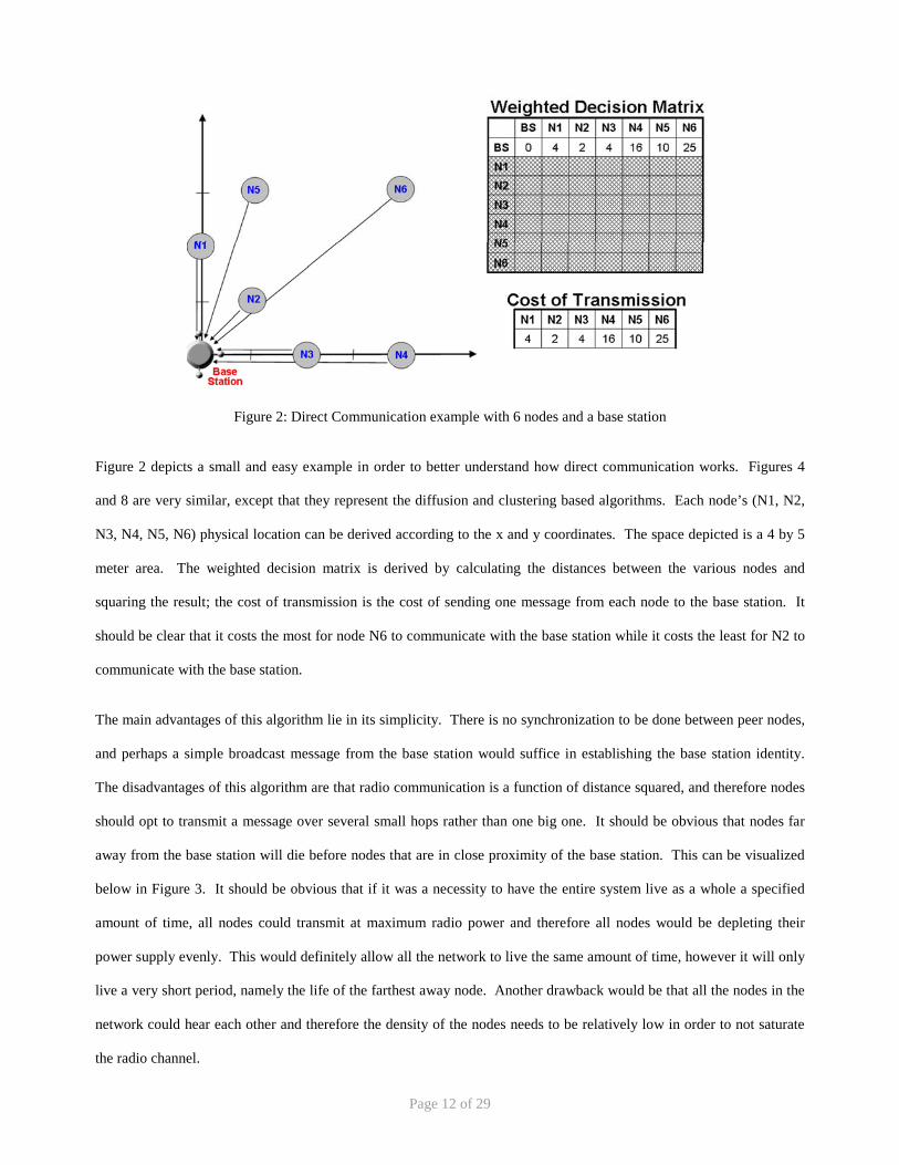
Figure 2: Direct Communication example with 6 nodes and a base station

Figure 2 depicts a small and easy example in order to better understand how direct communication works. Figures 4

and 8 are very similar, except that they represent the diffusion and clustering based algorithms. Each node’s (N1, N2,

N3, N4, N5, N6) physical location can be derived according to the x and y coordinates. The space depicted is a 4 by 5

meter area. The weighted decision matrix is derived by calculating the distances between the various nodes and

squaring the result; the cost of transmission is the cost of sending one message from each node to the base station. It

should be clear that it costs the most for node N6 to communicate with the base station while it costs the least for N2 to

communicate with the base station.

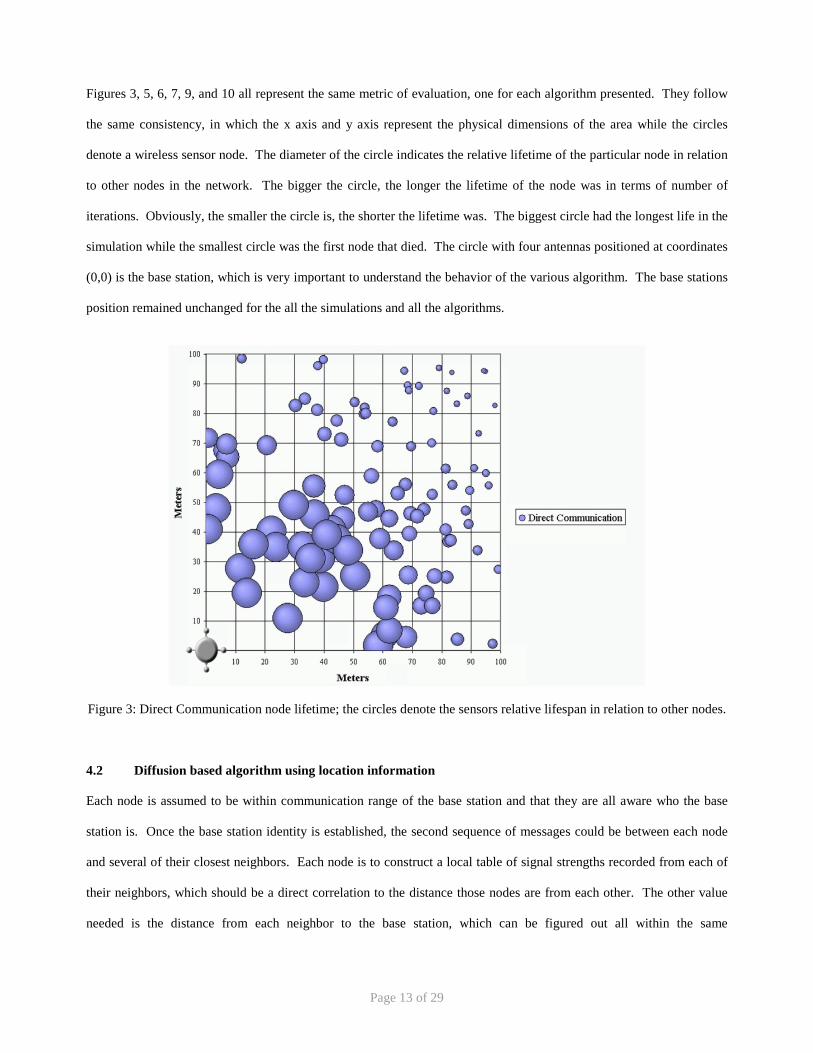
The main advantages of this algorithm lie in its simplicity. There is no synchronization to be done between peer nodes,

and perhaps a simple broadcast message from the base station would suffice in establishing the base station identity.

The disadvantages of this algorithm are that radio communication is a function of distance squared, and therefore nodes

should opt to transmit a message over several small hops rather than one big one. It should be obvious that nodes far

away from the base station will die before nodes that are in close proximity of the base station. This can be visualized

below in Figure 3. It should be obvious that if it was a necessity to have the entire system live as a whole a specified

amount of time, all nodes could transmit at maximum radio power and therefore all nodes would be depleting their

power supply evenly. This would definitely allow all the network to live the same amount of time, however it will only

live a very short period, namely the life of the farthest away node. Another drawback would be that all the nodes in the

network could hear each other and therefore the density of the nodes needs to be relatively low in order to not saturate

the radio channel.

of 29

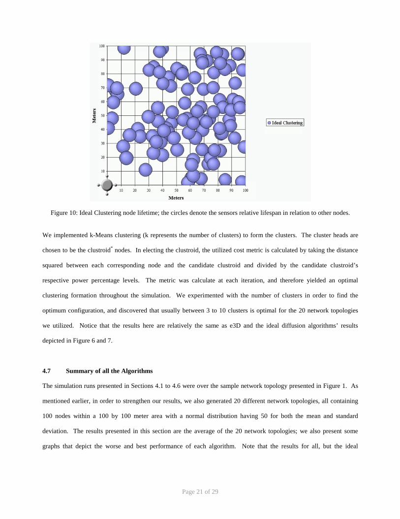
Figures 3, 5, 6, 7, 9, and 10 all represent the same metric of evaluation, one for each algorithm presented. They follow

the same consistency, in which the x axis and y axis represent the physical dimensions of the area while the circles

denote a wireless sensor node. The diameter of the circle indicates the relative lifetime of the particular node in relation

to other nodes in the network. The bigger the circle, the longer the lifetime of the node was in terms of number of

iterations. Obviously, the smaller the circle is, the shorter the lifetime was. The biggest circle had the longest life in the

simulation while the smallest circle was the first node that died. The circle with four antennas positioned at coordinates

(0,0) is the base station, which is very important to understand the behavior of the various algorithm. The base stations

position remained unchanged for the all the simulations and all the algorithms.

Figure 3: Direct Communication node lifetime; the circles denote the sensors relative lifespan in relation to other nodes.

4.2 Diffusion based algorithm using location information

Each node is assumed to be within communication range of the base station and that they are all aware who the base

station is. Once the base station identity is established, the second sequence of messages could be between each node

and several of their closest neighbors. Each node is to construct a local table of signal strengths recorded from each of

their neighbors, which should be a direct correlation to the distance those nodes are from each other. The other value

needed is the distance from each neighbor to the base station, which can be figured out all within the same

of 29

synchronization messages. This setup phase needs only be completed once at the startup of the system; therefore, it can

be considered as constant cost and should not affect the algorithm’s performance beyond the setup phase.

One important aspect needs to be brought out. If not careful in designing the algorithm, loops can form and hence

messages might never reach their intended destinations although power is continuously being dissipated as they are

forwarded in a never-ending cycle. In order to eliminate this possibility, we considered not only the distance from the

source to the candidate neighbor, but also from the candidate neighbor to the base station. If a simple test is made to

verify that the candidate neighbor is closer to the base station than the sending node, it should be obvious that any node

will always send messages a step closer towards the base station. Under no circumstance will a node ever send a

message in a backward direction. In the event that a node cannot find a suitable neighbor to transmit to that is closer to

the base station than itself, the sending node should chose the base station as its best neighbor.

The simulation assumes that each node transmits at a fixed rate, and always has data to transmit. In every iteration of

the simulation, each node sends its data that is destined for the base station, to the best neighbor. Each node acts as a

relay, merely forwarding every message received to its respective neighbor. The best neighbor is calculated using the

distance from the sender and the distance from the neighbor to the base station. This ensures that the data is always

flowing in the direction of the base station and that no loops are introduced in the system. Notice that the complete path

is not needed in order to calculate the best optimal neighbor to transmit to. Since each node makes the best decision for

itself at a local level, it is inferred that the system should be fairly optimized as a whole. Eventually, each node will

deplete its limited power supply and die. When all nodes are dead, the simulation terminates, and the system is said to

be dead.

Figure 4 depicts the simple example showing how diffusion defers from the direct communication. If Figure 2 and 4 are

compared, it should be obvious that although node N6 still has the highest cost of communication with the base station,

its cost is only 15 units while direct communication’s cost was 25 units.

The main advantage of this system is its fairly light complexity, which allows the synchronization of the neighboring

nodes to be done relatively inexpensive, and only once at the system startup. The system also distributes the lifetime of

the network a little bit more efficiently.

of 29

Figure 4: Diffusion Communication example with 6 nodes and a base station

The disadvantage of this system is that it still does not completely evenly distribute the energy dissipated since nodes

close to the base station will die far sooner before nodes far away from the base station. Notice that this phenomenon is

inversely proportional to the direct communication algorithm. It should be clear that this happens because the nodes

close to the base station end up routing many messages per iteration for the nodes farther away.

0

10

20

30

40

50

60

70

80

90

100

0 10 20 30 40 50 60 70 80 90 100

Meters

Met

ers

Basic Diffusion

Figure 5: Basic Diffusion node lifetime; the circles denote the sensors relative lifespan in relation to other nodes.

of 29

4.3 e3D: Diffusion based algorithm using location, power, and load as metrics

In addition to everything that the basic diffusion algorithm performs, each node makes a list of suitable neighbors and

ranks them in order of preference, similar to the previous approach. Every time that a node changes neighbors, the

sender will require an acknowledgement for its first message which will ensure that the receiving node is still alive. If a

time out occurs, the sending node will choose another neighbor to transmit to and the whole process repeats. Once

communication is initiated, there will be no more acknowledgements for any messages. Besides data messages, we

introduce exception messages which serve as explicit synchronization messages. Only receivers can issue exception

messages, and are primarily used to tell the sending node to stop sending and let the sender choose a different neighbor.

An exception message is generated in only three instances: the receiving node’s queue is too large, the receiver’s power

is less than the sender’s power, and the receiver has passed a certain threshold which means that it has very little power

left.

At any time throughout the system’s lifetime, a receiver can tell a sender not to transmit anymore because the receiver’s

queues are full. This should normally not happen, but in the event it does, an exception message would alleviate the

problem. In our current schema, once the sending node receives an exception message and removes his respective

neighbor off his neighbor list, the sending node will never consider that same neighbor again. We did this in order to

minimize the amount of control messages that would be needed to be exchanged between peer nodes. However, future

considerations could be to place a receiving neighbor on probation in the event of an exception message, and only

permanently remove it as a valid neighbor after a certain number of exception messages. The results were almost

unchanged when we applied this last change, and therefore we omitted it from our current implementation.

The second reason an exception message might be issued, which is the more likely one, is when the receiver’s power is

less than the sender’s power. If we allowed the receiver to send an exception message from the beginning based on this

test, most likely the receiver would over-react and tell the sender to stop sending although it is not clear that it was

really necessary. We therefore introduced a threshold for the receiver, in which if his own power is less than the

specified threshold, it would then analyze the receiving packets for the sender’s power levels. If the threshold was made

too small, then by the time the receiver managed to react and tell the sender to stop sending, too much of its power

supply had been depleted and its life expectancy thereafter would be very limited while the sending node’s life

expectance would be much longer due to its less energy consumption. Through empirical results, we concluded that the

of 29

optimum threshold is 45% of the receiver’s power levels when it in order to equally distribute the power dissipation

throughout the network.

In order to avoid having to acknowledge every message or even have heartbeat messages, we introduce an additional

threshold that will tell the receiving node when its battery supply is almost gone. This threshold should be relatively

small, in the 5~10% of total power, and is used for telling the senders that their neighbors are almost dead and that new

more suitable neighbors should be elected.

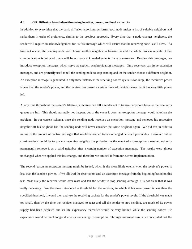
It should be clear that the synchronization cost of e3D is two messages for each pair of neighboring nodes. The rest of

the decisions will be based on local look-ups in its memory for the next best suitable neighbor to which it should

transmit to. Eventually, when all suitable neighbors are exhausted, the nodes opt to transmit directly to the base station.

By looking at the empirical results obtained, it is only towards the end of the system’s lifetime that the nodes decide to

send directly to the base station.

Figure 6: e3D Diffusion node lifetime; the circles denote the sensors relative lifespan in relation to other nodes.

The main advantage of this algorithm is the near perfect system lifetime in which most nodes in the network live

approximately the same duration. The system distributes the lifetime and load on the network much better than the

previous two approaches. The disadvantage when compared to of this algorithm is its higher complexity, which

of 29

requires some synchronization messages throughout the lifetime of the system. These synchronization message are very

few, and therefore worth the price in the event that the application calls for such strict performance.

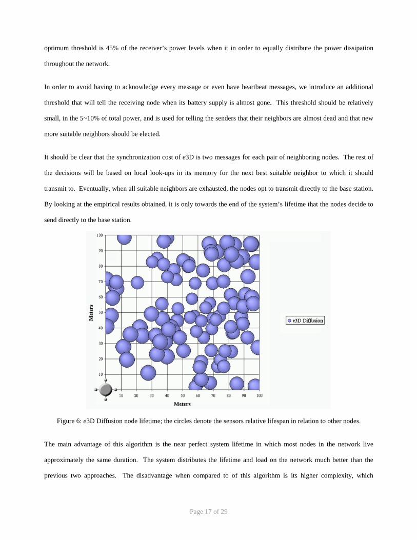
4.4 Ideal Diffusion Based Algorithm

With the ideal diffusion based routing algorithm, we attempt to show the upper bound on performance for the diffusion

based algorithms. We utilize all the assumptions and properties of the previous two algorithms. However, one major

difference is that all nodes are given global information about all other nodes with information such as power levels and

load information. Imagine having a directed acyclic tree with the base station as the root. The distance between the

nodes times the power levels at the receiver would be the cost for the particular edge. Each node is to find the best

neighbor at each iteration, which in principle involves reconstructing the tree at each iteration. Obviously this is almost

as hard to achieve in a real world implementation as the clustering techniques we will later discuss, however, the

findings here are relevant in order to see the ideal bound on performance for the diffusion based algorithms.

Figure 7: Ideal Diffusion node lifetime; the circles denote the sensors relative lifespan in relation to other nodes.

4.5 Random Clustering Based Algorithm

This algorithm is similar to LEACH, except there is no data aggregation at the cluster heads. The algorithm was

described in detail in Section 2.2, and therefore we forward the reader to that Section for details on the algorithm.

Random cluster heads are chosen and clusters of nodes are established which will communicate with the cluster heads.

of 29

The main advantage of this algorithm is the distribution of power dissipation achieved by randomly choosing the group

heads. This yields a random distribution of node deaths. The disadvantage of this algorithm is its relatively high

complexity, which requires many synchronization messages compared to e3D at regular intervals throughout the

lifetime of the system. Note that cluster heads should not be chosen at every iteration since the cost of synchronization

would be very large in comparison to the number of messages that would be actually transmitted. In our simulation, we

used rounds of 20 iterations between choosing new cluster heads. The high cost of this schema is not justifiable for the

performance gains over much simpler schemes such as direct communication. As a whole, the system does not live

very long and has similar characteristics to direct communication, as observed by our simulation in Figure 11. Notice

that the only difference in its perceived performance from direct communication is that it randomly kills nodes

throughout the network rather than having all the nodes die on one extreme of the network.

Figure 8 shows a brief example of how clustering works, but do not take the depicted example as the only way to cluster

the given six nodes. Suppose that node N1 and N3 were chosen as the cluster heads, then the corresponding

memberships would be as depicted below. The important concept to visualize is that node N2 needs to communicate

backwards to node N1 in order to communicate with the base station. This is an inevitable fact of clustering, regardless

whether it is randomly performed or not.

Figure 8: Clustering Communication example with 6 nodes and a base station; the * next to the nodes name indicates

that a particular node is chosen to be the cluster head.

of 29

Figure 9 shows how nodes with varying distances from the base station died throughout the network. The bigger circles

depicted below represent the nodes that lived the longest. The nodes that are farther away would tend to die earlier

because the cluster heads that are farther away have much more work to accomplish than cluster heads that are close to

the base station. It should be noted that the random clustering algorithm had a wide range of performance results, which

indicated that its performance was directly related to the random cluster election. As an interesting fact, the worst case

scenario had worse performance by a factor of ten in terms of overall system lifetime.

Figure 9: Random Clustering node lifetime; the circles denote the sensors relative lifespan in relation to other nodes.

4.6 Ideal Clustering Based Algorithm

We implemented this algorithm for comparison purposes to better evaluate the diffusion approach, especially that the

random clustering algorithm had a wide range of performance results since everything depended on the random cluster

election. The cost of implementing this classical clustering algorithm in a real world distributed system such as wireless

sensor networks is energy prohibitively high; however, it does offer us insight into the upper bounds on the performance

of clustering based algorithms.

of 29

Figure 10: Ideal Clustering node lifetime; the circles denote the sensors relative lifespan in relation to other nodes.

We implemented k-Means clustering (k represents the number of clusters) to form the clusters. The cluster heads are

chosen to be the clustroid* nodes. In electing the clustroid, the utilized cost metric is calculated by taking the distance

squared between each corresponding node and the candidate clustroid and divided by the candidate clustroid’s

respective power percentage levels. The metric was calculate at each iteration, and therefore yielded an optimal

clustering formation throughout the simulation. We experimented with the number of clusters in order to find the

optimum configuration, and discovered that usually between 3 to 10 clusters is optimal for the 20 network topologies

we utilized. Notice that the results here are relatively the same as e3D and the ideal diffusion algorithms’ results

depicted in Figure 6 and 7.

4.7 Summary of all the Algorithms

The simulation runs presented in Sections 4.1 to 4.6 were over the sample network topology presented in Figure 1. As

mentioned earlier, in order to strengthen our results, we also generated 20 different network topologies, all containing

100 nodes within a 100 by 100 meter area with a normal distribution having 50 for both the mean and standard

deviation. The results presented in this section are the average of the 20 network topologies; we also present some

graphs that depict the worse and best performance of each algorithm. Note that the results for all, but the ideal

of 29

algorithms include the setup costs and synchronization costs. The cost of synchronization was omitted for the ideal case

algorithms because the cost of synchronization would have overshadowed the results; furthermore, the ideal algorithms

are not realistic and therefore we only interested on the upper bound they represented.

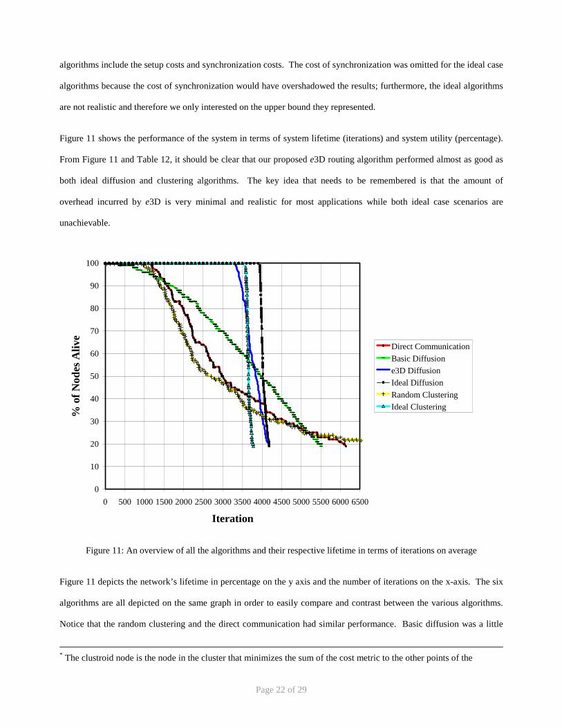
Figure 11 shows the performance of the system in terms of system lifetime (iterations) and system utility (percentage).

From Figure 11 and Table 12, it should be clear that our proposed e3D routing algorithm performed almost as good as

both ideal diffusion and clustering algorithms. The key idea that needs to be remembered is that the amount of

overhead incurred by e3D is very minimal and realistic for most applications while both ideal case scenarios are

unachievable.

0

10

20

30

40

50

60

70

80

90

100

0 500 1000 1500 2000 2500 3000 3500 4000 4500 5000 5500 6000 6500

Iteration

% o

f Nod

es A

live

Direct CommunicationBasic Diffusione3D DiffusionIdeal DiffusionRandom ClusteringIdeal Clustering

Figure 11: An overview of all the algorithms and their respective lifetime in terms of iterations on average

Figure 11 depicts the network’s lifetime in percentage on the y axis and the number of iterations on the x-axis. The six

algorithms are all depicted on the same graph in order to easily compare and contrast between the various algorithms.

Notice that the random clustering and the direct communication had similar performance. Basic diffusion was a little

* The clustroid node is the node in the cluster that minimizes the sum of the cost metric to the other points of the

of 29

better, but had an overall similar performance characteristic as direct and random clustering. The remaining three

algorithms, e3D, the ideal diffusion, and the ideal clustering algorithms, all performed relatively similar. e3D was

expected to not outperform both ideal cases since it used a realistic scheme for the number of synchronization messages.

The ideal diffusion algorithm was also expected to perform better than the ideal clustering since the clustering algorithm

cannot avoid sending some message from some nodes backward as they travel from the source to the cluster head and to

their final destination at the base station. It should be clear that since the clustering approach spends more energy in

transmitting a message from the source to the destination, the overall system lifetime cannot be expected to be longer

than the lifetime represented by the ideal diffusion, in which each source sends the corresponding message along the

ideal path towards the base station. Lastly, notice the sharp drop in the percentage of nodes alive, which indicates that

the algorithms (e3D, ideal diffusion, and ideal clustering) evenly distribute the power dissipated during communication

regardless of node location.

0

10

20

30

40

50

60

70

80

90

100

0 500 1000 1500 2000 2500 3000 3500 4000 4500 5000 5500 6000 6500

Iteration

% o

f Nod

es A

live


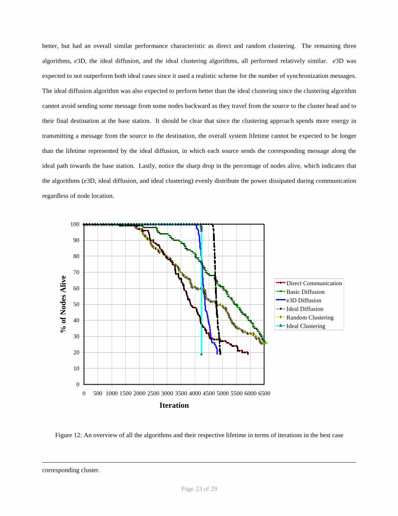
Figure 12: An overview of all the algorithms and their respective lifetime in terms of iterations in the best case

corresponding cluster.

of 29

In order to further strengthen our results, we have isolated the best and worst case performance of each algorithm based

on the various network topologies. The best case scenario is presented in Figure 12 while the worst case scenario is

presented in Figure 13.

0

10

20

30

40

50

60

70

80

90

100

0 500 1000 1500 2000 2500 3000 3500 4000 4500 5000 5500 6000 6500

Iteration

% o

f Nod

es A

live


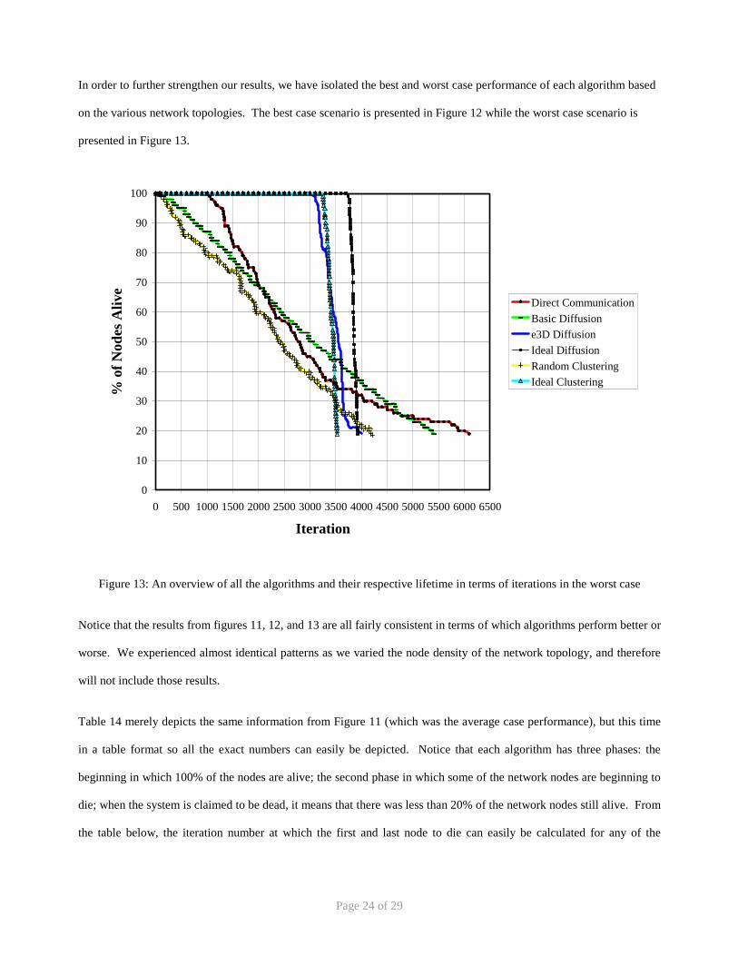
Figure 13: An overview of all the algorithms and their respective lifetime in terms of iterations in the worst case

Notice that the results from figures 11, 12, and 13 are all fairly consistent in terms of which algorithms perform better or

worse. We experienced almost identical patterns as we varied the node density of the network topology, and therefore

will not include those results.

Table 14 merely depicts the same information from Figure 11 (which was the average case performance), but this time

in a table format so all the exact numbers can easily be depicted. Notice that each algorithm has three phases: the

beginning in which 100% of the nodes are alive; the second phase in which some of the network nodes are beginning to

die; when the system is claimed to be dead, it means that there was less than 20% of the network nodes still alive. From

the table below, the iteration number at which the first and last node to die can easily be calculated for any of the

of 29

algorithms. The first node died at the iteration where 99% of the nodes are still alive for each respective algorithm. The

last node died at the first occurrence of the word “dead” in the table below.

Iteration # 375 984 1196 3329 3582 3780 3944 4173 4185 5507 6140 6952

Direct 100% 100% 99% 45% 42% 41% 39% 34% 34% 23% Dead Dead

Diffusion 99% 97% 95% 64% 59% 55% 51% 47% 46% Dead Dead Dead

E3D 100% 100% 100% 99% 80% 55% 40% Dead Dead Dead Dead Dead

Ideal Diffusion 100% 100% 100% 100% 100% 100% 99% 22% Dead Dead Dead Dead

Random Clustering 100% 99% 97% 43% 37% 35% 34% 32% 31% 24% 22% Dead

Ideal Clustering 100% 100% 100% 100% 99% Dead Dead Dead Dead Dead Dead Dead

Table 14: An overview of all the algorithms and their respective lifetime in terms of iterations

Table 15 attempts to capture an overview comparison between our simulation results and other proposed algorithms

presented in [8, 9]. The algorithm names in Error! Reference source not found. are briefly described below. For a

complete description of each algorithm, please refer to [8, 9].

• Direct: direct communication between each node and the base station

• Leach: clustering-based protocol that utilizes randomized rotation of cluster heads to collect data from neighboring

nodes, aggregate data, and send it to the base station

• Pegasis: chain-based protocol, in which group heads are chosen randomly and each node communicates only with a

close neighbor forming a chain leading to its cluster head, and onto the base station

• MTE: each node sends to the closest neighbor on the way to the base station solely based on spatial information

(naïve diffusion as we have described it earlier)

• Static Clustering: Same as Leach, but with the cluster heads chosen apriori

• Direct, Diffusion, e3D, Ideal Diffusion, Random Clustering, and Ideal Clustering are the algorithms that were

implemented and tested in our simulation.

The comparisons in Table 15 show the iterations when the first and last node died. Note that the proposed system lived

nearly 80% of its lifetime with 100% utility. The number of iterations each algorithm lasted before the first and last

node died should not be compared among the various algorithms since all these results were extracted from various

works [8, 9] and this paper. Each paper had their own assumptions about the node characteristics

(transmit/receive/amplification power dissipation), and therefore the wide range of system lifetimes. What should be

of 29

evident is the percentage of time each algorithm allowed the network to operate at 100% utility. Some of the related

work might have had larger system utility (number of iterations while the system had 100% of the nodes alive) because

of the use of the unrealistic aggregation scheme which allowed each forwarding node to aggregate unlimited number of

incoming packets to one outgoing packets. This in principle placed much less stress on forwarding nodes (cluster

heads, neighbors, etc…) and therefore they obtained somewhat better results. Although no aggregation (data fusion)

schemes are used in e3D, it achieves almost 80% system utility, much higher than other related work and other

algorithms we implemented.

Algorithm Name

First Node Dies

Last Node Dies

% of System Lifetime with 100% utility

Direct [9] 56 122 45.90%

Leach [9] 690 1077 64.07%

Pegasis [9] 1346 3076 43.76%

Direct [8] 217 468 46.37%

MTE [8] 15 843 1.78% Static

Clustering [8] 106 240 44.17%

LEACH [8] 1848 2608 70.86%

Direct 1196 6140 19.48%

Diffusion 375 5507 6.80%

e3D 3329 4173 79.77%

Ideal Diffusion 3944 4185 94.24% Random

Clustering 984 6952 14.15%

Ideal Clustering 3582 3780 94.76% Table 15: Summary view of various algorithms from related work and our work

One last important metric to examine is the synchronization cost for each of the discussed algorithms. Table 16 depicts

the time complexity in relation to network size (n), iterations of system life (i), and some constant (c).

Each of the algorithms we examined had similar initial setup costs, except for the direct communication which only

required the base station to advertise itself with a broadcast message. The other algorithms all required that each node

in the network broadcast one message. In terms of maintenance synchronization costs, the direct communication

algorithm has no cost. The diffusion algorithm has a cost of n total unicast messages that are sent to the sender when

receiver’s power is too depleted to receive any more messages. The e3D algorithm is similar, however it also has some

other times (various thresholds) when it sends control unicast messages to the senders; note that the constant c is

of 29

relatively small (eg. 2~3). In the ideal diffusion, each node broadcasts control messages at every iteration, and therefore

we have the complexity of O(n*i). Note that there are only n*I messages in total that are being transmitted, and

therefore having a complexity of O(n*i) of broadcasted messages is prohibitively expensive. The random clustering

complexity is O(ln(n)*i/c). ln(n) is derived from the number of cluster heads, which from experimental results and the

related work, seems to hold true. In our simulation, c was set to 20 as new cluster heads were chosen every 20

iterations. In the ideal clustering approach, some entity must collect information about all nodes in the network, figure

out the ideal clusters at that moment in time, and communicate back to each node which cluster they belong to; this

entire process must done at each iteration, and thus we came up to O(n*i*c).

Algorithm Name

SynchronizationComplexity

Direct None

Diffusion O(n)

e3D O(c*n)

Ideal Diffusion O(n*i) Random

Clustering O(ln(n)*i/c)

Ideal Clustering O(n*i*c) Table 16: Synchronization complexity for the examined algorithms

5.0 CONCLUSION AND FUTURE WORK

Due to space constraints, we were not able to include all experimental results we have obtained, but we did present the

most relevant information to compare e3D with other proposed algorithms that had similar goals to ours. The proposed

algorithm (e3D) performed well in terms of achieving its goal to evenly distribute the power dissipation throughout the

network while not creating a very large burden for synchronization purposes.

Our simulation results seem very promising. By distributing the power usage and load on the network, we are

essentially improving the quality of the network and making maintenance of it much simpler, since the network lifetime

will be predictable as a whole, rather than on a node-by-node basis. In summary, we showed that energy-efficient

distributed dynamic diffusion routing is possible at very little overhead cost. The most significant outcome is the near

optimal performance of e3D when compared to its ideal counterpart in which global knowledge is assumed between the

network nodes.

of 29

Therefore, we conclude that complex clustering techniques are not necessary in order to achieve good load and power

usage balancing. Previous work suggested random clustering as a cheaper alternative to traditional clustering; however,

random clustering cannot guarantee good performance according to our simulation results. Perhaps, if aggregation (data

fusion) is used, random clustering might be a viable alternative.

Since e3D only addressed static networks, in future work, we will investigate possible modifications so it could support

mobility support, and therefore have a wider applicability. We will address the possible aggregation schemes in a future

paper in which we discuss in detail both realistic and unrealistic aggregation schemes in order to make the proposed

algorithm suitable for most applications. Eventually, it would be nice to implement these algorithms using the Rene RF

motes in order to strengthen the simulation results.

6.0 REFERENCES

[1] J. M. Rabaey, M. J. Ammer, J. L. da Silva, D. Patel, S. Roundy, “PicoRadio Supports Ad Hoc Ultra-Low Power

Wireless Networking.”

[2] D. Estrin, R. Govindan, J. Heidemann, and Satish Kumar, “Next Century Challenges: Scalable Coordination in

Sensor Networks”, Proceedings of Mobicom ’99, 1999.

[3] R. Pichna and Q. Wang, “Power Control”, The Mobile Communications Handbook. CRC Press, 1996, pp. 370-

30.

[4] R. Ramanathan and R. Hain, “Topology Control of Multihop Wireless Networks Using Transmit Power

Adjustment”, Proceeding Infocom 2000, 2000.

[5] W. Mangione-Smith and P.S. Ghang, “A Low Power Medium Access Control Protocol for Portable Multimedia

Systems”, In Proceeding 3rd Intl. Workshop on Mobile Multimedia Communications, Princeton, NJ, Sept. 25-27,

1996.

[6] K. M. Sivalingam, M.B. and P. Agrawal, “Low Power Link and Access Protocols for Wireless Multimedia

Networks”, Proceedings IEEE Vehicular Technology Conference VTC’97, May 1997.

of 29

[7] M. Stemm, P. Gauther, D. Harada and R. Katz, “Reducing Power Consumption of Network Interfaces in Hand-

Held Devices”, Proceedings 3rd Intl. Workshop on Mobile Multimedia Communications, Sept. 25-27, 1996,

Princeton, NJ.

[8] W. Heinzelman, A. Chandrakasan, and H. Balakrishnan, “Energy-Efficient Communication Protocol for Wireless

Microsensor Networks”, Hawaiian Int'l Conf. on Systems Science, January 2000.

[9] S. Lindsey and C. Raghavendra, “PEGASIS:Power-Efficient GAthering in Sensor Information Systems”,

International Conference on Communications, 2001.

[10] I. Raicu, O. Richter, L. Schwiebert, S. Zeadally, “Using Wireless Sensor Networks to Narrow the Gap between

Low-Level Information and Context-Awareness”, ISCA 17th International Conference on Computers and Their

Applications, CATA 2002.

[11] A. K. Jain, R. C. Dubes, “Algorithm for Clustering Data,” Prentice Halls, 1988, pp. 1.

[12] J. Hill, R. Szewczyk, A. Woo, S. Hollar, D. Culler, K. Pister, “System architecture directions for network

sensors”, ASPLOS 2000.

[13] A. S. Tanenbaum, Computer Networks, Third Edition, Prentice Hall Inc., 1996, pp. 276-287.

[14] G Coulouris, J. Dollimore, T. Kindberg, Distributed Systems, Concept and Design, Third Edition, Addison-

Wesley Publishers Limited, 2001, pp. 116-119.

[15] C. Intanagonwiwat, R. Govindan and D. Estrin, “Directed diffusion: A scalable and robust communication

paradigm for sensor networks”, Proceedings of the Sixth Annual International Conference on Mobile Computing

and Networking (MobiCOM '00), August 2000, Boston, Massachussetts.

Energy-Efficient Routing Algorithms in Wireless Sensor...

Documents

Transcript of Energy-Efficient Routing Algorithms in Wireless Sensor...