Energy-Efﬁcient Accelerator Design for Deformable ...

1

Energy-Efficient Accelerator Design for DeformableConvolution NetworksDawen Xu, Cheng Chu, Cheng Liu, Ying Wang,

Huawei Li, Senior Member, IEEE, Xiaowei Li, Kwang-Ting Cheng, Fellow, IEEE

Abstract—Deformable convolution networks (DCNs) proposedto address the image recognition with geometric or photometricvariations typically involve deformable convolution that con-volves on arbitrary locations of input features. The locationschange with different inputs and induce considerable dynamicand irregular memory accesses which cannot be handled byclassic neural network accelerators (NNAs). Moreover, bilinearinterpolation (BLI) operation that is required to obtain deformedfeatures in DCNs also cannot be deployed on existing NNAsdirectly. Although a general purposed processor (GPP) seatedalong with classic NNAs can process the deformable convolution,the processing on GPP can be extremely slow due to the lack ofparallel computing capability.

To address the problem, we develop a DCN accelerator onexisting NNAs to support both the standard convolution and de-formable convolution. Specifically, for the dynamic and irregularaccesses in DCNs, we have both the input and output featuresdivided into tiles and build a tile dependency table (TDT) totrack the irregular tile dependency at runtime. With the TDT, wefurther develop an on-chip tile scheduler to handle the dynamicand irregular accesses efficiently. In addition, we propose anovel mapping strategy to enable parallel BLI processing onNNAs and apply layer fusion techniques for more energy-efficientDCN processing. According to our experiments, the proposedaccelerator achieves orders of magnitude higher performance andenergy efficiency compared to the typical computing architecturesincluding ARM, ARM+TPU, and GPU with 6.6% chip areapenalty to a classic NNA.

Index Terms—Deformable Convolution Network, Neural Net-work Accelerator, Irregular Memory Access, Runtime TileScheduling

I. INTRODUCTION

Deformable convolution network (DCN) [1], a new cate-gory of neural networks, is proposed to address the neuralnetwork model accuracy degradation caused by geometric andphotometric variations such as lighting and rotation occurredin many practical applications like medical imaging. DCNstypically sample arbitrary locations of the input features forthe convolution such that the objects with different scalesor deformation can be captured. The sampling patterns ofdeformable convolution can be learned and calculated using

Corresponding author: Cheng LiuDawen Xu and Cheng Chu are with both Hefei University of Technology, An-hui, 230009 and Institute of Computing Technology (ICT), Chinese Academyof Sciences (CAS), Beijing, China, 100180.Cheng Liu, Ying Wang, Huawei Li and Xiaowei Li are with ICT, CAS,Beijing, China, 100180. (E-mail: [email protected])Kwang-Ting Cheng is with Department of Computer Science and Engineering,The Hong Kong University of Science and Technology, Hong Kong.(E-mail:[email protected])

an additional convolution layer. With the unique deformableconvolution, DCNs have shown superior performance on manyvision tasks such as object detection [1] [2] [3] [4], semanticsegmentation [1] [5] [6] [7] and classification [8] [9] [10]. Forinstance, the authors in [1] demonstrated that the predictionaccuracy of the proposed DCN increases from 70% to 75%on the image semantic segmentation dataset (CityScapes).Significant prediction accuracy improvement is also observedin human motion recognition task [11] [12], action detectiontask [13] [14] and intelligent medical monitoring and treatment[15] [16].

Despite the great advantages, each deformable convolu-tion operation in DCNs needs additional convolution-basedindex1 calculation and bilinear interpolation (BLI) to obtaindeformed features other than a standard convolution, so itis both computing- and memory-intensive and requires in-tensive acceleration for widespread deployment. Nevertheless,DCNs can not be deployed on conventional neural networkaccelerators mainly from the following two aspects. First, itconvolves on arbitrary locations of the input features insteadof fixed sliding windows as depicted in Figure 1. The locationsi.e. the indices to the input features are generated at runtimeand they will cause both dynamic and irregular accesses tothe memory, which can not be fitted to conventional neuralnetwork accelerators targeting at regular memory accesses anddata flows. Second, DCNs have a standard convolution tocalculate the indices, but the calculated indices are usuallynot integers and can not be used to retrieve the feature datadirectly. Typically, BLI algorithm is utilized to approximatethe features with the nearest original input features. Thisstep is also not supported in conventional neural networkaccelerators. An intuitive solution to execute DCNs is toconduct the deformable convolution on a general purposedprocessor (GPP) which is usually seated with a neural networkaccelerator while deploying the rest of the normal neuralnetwork operations in DCNs on a neural network accelerator.However, GPPs especially the embedded processors withlimited parallel processing capability is inefficient for thebilinear interpolation, and a large number of irregular memoryaccesses and data transfers between the GPPs and the neuralnetwork accelerator also inhibit the DCN execution efficiency

1’offset’ is used to represent the relative distance to sliding windowpositions of a standard convolution in many DCNs. However, it is inconvenientto retrieve the features with the random offsets in hardware and offsets need tobe converted to indices of the features instead. While the conversion is trivial,we use index in both the algorithm description and hardware description tomake the notation consistent across the paper.

arX

iv:2

107.

0254

7v1

[cs

.AR

] 6

Jul

202

1

2

ConvolutionReorganized

indices

Input feature Output feature

Convolution

IndicesInput feature Deformed feature Output feature

1

BLI Convolution

(b)

(a)

1 2 3

(b) (c)

Deformed sampling

location

Regular sampling

location

2

3 4

Fig. 1. Deformable convolution (a) regular sliding window in a standard convolution, (b) irregular sampling of a deformable convolution, (c) deformableconvolution processing.

dramatically.Recently, there are also works proposed to revise the DCN

models to fit existing neural network accelerators. The authorsin [17] proposed to replace the bilinear interpolation algorithmwith a simple rounding strategy and restrict the samplinglocations to avoid dynamic memory access induced bufferingproblems. Similarly, the authors in [18] also proposed tomodify the DCN models to reduce the receptive field sizesubstantially so that the sampling locations are limited to asmall region, which avoids the dynamic memory accessesacross the whole input feature map. Although these approachesare demonstrated to be effective on existing neural networkaccelerators with minor model accuracy, it essentially poseshardware constraints to the model design and particularly lim-its its use on scenarios that are sensitive to the model accuracyloss. In addition, it requires time-consuming retraining andtraining data that may not be applicable to the end users.Thereby, we investigate the computing of the DCNs and seekto implement the entire unmodified deformable convolution ontop of a unified neural network accelerator directly.

To implement the entire DCNs on a unified accelerator andreuse the conventional neural network accelerator as muchas possible, we revisit a typical neural network acceleratorarchitecture mainly for the new irregular feature sampling andthe BLI required by DCNs. For the dynamic and irregularfeature accesses, we observe that the input data required bythe deformable convolutional output is imbalanced and someof the input features are utilized more than the others. Moredetails can be found in Section III. With this observation, wepropose to divide the input and output features into smallertiles and build a tile dependency table (TDT) that keeps arecord of all the required input tile IDs of each output tile withruntime tracking. On top of the TDT, we further schedule theoutput tile execution such that the buffered tiles are reused asmuch as possible and the overall memory access efficiencycan be improved. For the BLI, we convert it to multiplesmall vector-based dot production which can be mapped inparallel to the 2D computing array in typical neural networkaccelerators efficiently with a weight stationary data flow [19].In addition, we fuse the BLI and the following convolution tofurther reduce the intermediate data transmission between on-chip buffers and the external memory. With the proposed re-designing on top of a conventional neural network accelerator,the entire deformable convolution can be implemented on therevisited accelerator efficiently. According to our experiments

on a set of DCNs, it achieves orders of magnitude higherperformance and energy efficiency when compared to typicalcomputing architectures including ARM, ARM+TPU, andGPU while it incurs only minor hardware resource consump-tion compared to a conventional neural network accelerator.

The rest of the paper is organized as follows. In Section II,we introduce the typical deformable convolutional networksand formulate them into a unified computing model. Mean-while, we brief prior works about neural network acceleratorredesigning for new types of neural network models. In Sec-tion III, we characterize the computing patterns and memoryaccesses of deformable convolution. In Section IV, we showthe detailed design and optimizations of an accelerator forDCNs on top of a classical neural network accelerator. InSection V, we evaluate the performance and energy efficiencyof the accelerator and compare it with typical embeddedcomputing platforms. In Section VI, we conclude this work.

II. BACKGROUND AND RELATED WORK

A. Deformable convolutional networks

Deformable convolution may sample arbitrary locations ofthe input features for convolution such that it can capturethe objects with scale or transformation. The unique featuremakes it attractive in visual recognition tasks with geometricvariations such as lighting and rotation. There have beenmany deformable convolution architectures proposed recently[1], [14]. They typically include two standard convolutionoperations. The first convolution calculates the indices for theinput feature sampling while the second convolution convolveson the sampled features. Usually, a BLI operation is usedto bridge the two convolution operations. It approximates theinput features based on the non-integer indices generated bythe first convolution and provides the features as inputs to thesecond convolution. The structures of DCNs mainly differ onthe index reuse and can be roughly divided into two categories.The first category of DCNs has a unique index for each data inthe feature plane and the indices are reused across the differentchannels [14]. The second category of DCNs also has theindices shared across the feature channels, but it has a uniqueindex for each data in each convolution window [1]. Basically,the same data in the feature plane has different indices whenit is located in different convolution windows. The secondcategory of DCNs requires a larger convolution to calculatemore sampling indices and produces more deformed features

3

Fig. 2. Bilinear interpolation

than the first category of DCNs. The two categories of DCNsare abbreviated as DCN-I and DCN-II respectively.

B. Unified deformable convolution modelThe different deformable convolution can be represented

in a unified model as formulated in Equation 1-3. Basically,it has a convolution to determine the deformed locations orindices of the input features in the first step. This step isformulated in Equation 1 where c, l, i, j refer to input channelindex, output channel index, kernel offset in X dimension andkernel offset in Y dimension respectively. Since the indicescan be different when the feature data is in different positionsof the convolution kernel, we have yL, a vector of planarcoordinates with length L = 2 × K × K where K is thekernel size to represent the indices. Suppose αm and βn are thecorresponding coordinates in X axis and Y axis respectively.αm and βn are not integers, so they can not be used to retrievethe input features directly for the deformable convolution.To that end, a bilinear interpolation approach is utilized tocalculate the deformed features using the neighboring fea-tures around the location (αm, βn) in the second step. Thecalculated feature x

′

c,αm,βncan be obtained using Equation

2 where BLI(.) refers to the bilinear interpolation function,∆αm = αm − bαmc and ∆βm = βm − bβmc. A vividdescription of the BLI function can be found in Figure 2.When the input features are retrieved and organized accordingto the deformed indices, the deformable convolution can beobtained using a standard convolution over the reorganizedfeatures as shown in Equation 3 in the third step.

yL =∑c

∑i,j

wc,l,i,j · xc,i,j + bl (1)

x′

c,αm,βn= FBLI(xbαmc,bβnc, xbαmc,dβne, xdαme,bβnc,

xdαme,dβne,∆αm,∆βn)

= (1−∆αm) (1−∆βn)xbαmc,bβnc

+ (1−∆αm) ∆βnxbαmc,dβne

+ ∆αm (1−∆βn)xdαme,bβnc

+ ∆αm∆βnxdαme,dβne

(2)

y′

L′ =∑c

∑m,n

w′

c,l′ ,m,n· x

′

c,m,n + bl′ (3)

C. Neural Network Accelerator RedesigningThe great success of neural networks in massive domains

of applications inspires considerable efforts devoted to devel-oping neural network accelerators [20] [21] [22] [23] [24][25]. In spite of the notable efforts, newer network operationsproposed for higher performance may go beyond the capabilityof the existing neural network accelerators. Although it isusually possible to offload the unsupported operations to theattached GPPs while leaving the rest of the conventional neuralnetwork operations on the accelerator, the performance of theco-designed implementation may drop dramatically due to themassive data communication between GPP and the accelerator.Also complex operations offloaded to GPPs may still becomethe performance bottleneck due to the insufficient computingcapability of GPP and degrade the overall neural networkexecution. Thereby, the neural network accelerators are usuallyredesigned to meet the requirements of the new neural networkoperations on top of the existing neural network accelerators.For instance, unified neural network accelerators are also pro-posed to perform deconvolution used in generative adversarialneural networks other than the conventional convolution [26][27] [28] [29]. A novel accelerator is developed to support3D neural networks in [30] [31] [32]. The authors in [33]proposed to add a bilinear interpolation calculation moduleto an existing ReRAM neural network accelerator to enablein-situ DCN calculation. Inspired by prior works, we also tryto convert the deformable convolution to operations that canbe mapped to the neural network accelerator efficiently withminor hardware modification such that the whole deformableconvolution can be executed on the neural network acceleratorefficiently.

III. OBSERVATION

Since deformable convolution has many irregular memoryaccesses involved which dramatically affect the processingefficiency, we investigate the memory accesses of a typicaldeformable convolution in this section. We take the third con-volution layer of VGG16 as the basis of a typical deformableconvolution operation. As the memory accesses vary on differ-ent inputs, we randomly selected 2000 images from ImageNetand averaged the memory accesses for the investigation.

Figure 3 (a) shows the distribution of the input featureaccesses. Unlike standard convolution that usually has nearlyuniform utilization of the input features, deformable convolu-tion has distinct utilization of the different input features. Withthe 3×3 kernel used in the convolution, each input feature willbe utilized around 9 times. For the corresponding deformableconvolution, the access distribution shows dramatic difference.Around 15% of the features will be utilized by more than 12times, which take up around 25% of the feature accesses. Incontrast, more than 22% of the features are utilized less than 6times. While the neural networks can usually be tiled and thememory accesses can be performed in the granularity of a tile,we further analyze the input feature tile access distribution. Inthis experiment, we had both the input feature map and theoutput feature map divided into 25 tiles as an example. Thetile access distribution is shown in Figure 3 (b). It can beobserved that the input tile reuse still shows notable variation.

4

(a) Illustration of feature access statistics (b) Illustration of tile access statistics

(a) Feature access distribution

(b) Tile access distribution

0%

20%

40%

60%

80%

100%

0%

5%

10%

15%

0 5 10 15 20 25 30 35

Acc

um

ula

ted P

erce

nta

ge

Per

cen

tage

Feature PercentageAccumulated Feature Access PercentageAccumulated Feature Percentage

0%

20%

40%

60%

80%

100%

0%

5%

10%

15%

20%

0 2 4 6 8 10 12 14 16 18 20 22

Acc

um

ula

ted P

erce

nta

ge

Per

centa

ge

Tile Access PercentageAccumulated Tile Access PercentageAccumulated Tile Percentage

0%

20%

40%

60%

80%

100%

0%

5%

10%

15%

0 5 10 15 20 25 30 35

Acc

um

ula

ted

Per

cen

tag

e

Per

cen

tag

eFeature Percentage Accumulated Feature Access Percentage

Accumulated Feature Percentage

0%

20%

40%

60%

80%

100%

0%

5%

10%

15%

20%

0 2 4 6 8 10 12 14 16 18 20 22

Acc

um

ula

ted

Per

cen

tag

e

Per

cen

tag

e

Tile Access Percentage Accumulated Tile Access Percentage

Accumulated Tile Percentage

Fig. 3. Memory access characterization of the deformable convolution

In summary, the input features are not evenly accessed,so some of the input features are more likely to be reusedthan the other. Given limited on-chip buffers, scheduling theorder of the output feature calculation and optimizing theorder of the input feature accesses can potentially improve theon-chip buffer utilization and remains demanded for higherperformance and energy efficiency of the DCN processing.

IV. DCN ACCELERATOR ARCHITECTURE

A. Overall Accelerator Architecture

Deformable convolution is the major barrier that hinders thedeployment of DCNs on existing neural network accelerators.Thereby, taming the deformable convolution to the existingneural network accelerators is key to accelerate DCNs. Asformulated in Section II-B, deformable convolution consistsof three processing stages including convolution, BLI, andconvolution. Since the convolution operations in DCNs canbe deployed on existing neural network accelerators directly,the major challenge of DCN acceleration is to optimize theBLI operation that samples the input features according to theirregular indices calculated with the first convolution in DCNsand conducts the BLI calculation based on the sampled inputfeatures. Since the indices depend on the input features andthus change at runtime, the BLI sampling leads to complicatememory accesses. To address this dynamic and irregular mem-ory access problem, we have BLI divided into tiles and trackthe tile dependency at runtime with a tile dependency table(TDT). On top of the TDT, we have a tile scheduler to decidethe order of the output tile execution and the input tile loadingat the same time such that the tiles loaded to the on-chipbuffers can be fully utilized and the memory accesses to theexternal memory can be reduced. As for the BLI calculation,we reorganize it to multiple small vector-based dot productionand have the processing performed in parallel on top of the2D computing array in the neural network accelerator for thesake of higher performance.

Register

cnt

cnt

SUM

Comp

DMA

DMA

weight buffer

Input bufferDMA

output buffer

DMA

Initial index buffer

Controller

Instruction buffer

Swap

Off

-chip

mem

ory

Addr converter

ROI block sort

Addr converter

PE array

complete

Buffer addr

BLI coefficients

DMA

DMA

Input buffer

Weight buffer DMA

Output buffer

DMA

index buffer

Controller

Instruction buffer

Swap

Off

-chip

mem

ory

Address converter

Tile dependency

table

Buffer addr

BLI coefficients

PE

PE

PE

PE

PE

PE

PE

PE

PE

Data： Control： Indices：

01

10

01

Data：

Control：

Indices：

Coefficient

calculation

Scheduler

Fig. 4. DCN accelerator overview. The blocks filled with grey are addedspecifically for the deformable convolution processing while the rest of theblocks remain the same with a conventional neural network accelerator with2D computing array.

The proposed DCN accelerator architecture is shown inFigure 4. The components without filling any color belongto a classic neural network accelerator while the rest of thecomponents filled with grey are designed specially for thedeformable convolution. The entire accelerator is generallycontrolled with a sequence of instructions compiled fromthe target neural networks. The instructions are stored in theinstruction buffer and decoded at runtime to generate controlsignals for the entire accelerator. With the controlling, neuralnetwork operations are mapped and executed on the regular2D computing array. For the convolution operations, weightsfrom different filters are streamed to the different columnsof the computing array from top to bottom in parallel whileinput features are streamed from left to right in different rowsaccording to the output stationary data flow proposed in [19].

For the deformable convolution, it is divided into threedependent operations. The first convolution operation startswhen inputs and weights are ready in the on-chip buffers.The outputs of the first convolution are indices and will beutilized to sample from the input features. Since they are notintegers and can not be utilized to retrieve the input featuresdirectly, we have them stored in an index buffer and havean address converter to obtain the four neighboring integerindices. Meanwhile, BLI coefficients as proposed in SectionII-B are generated with a coefficient calculation block at thesame time. To this end, we can start the BLI calculation withthe retrieved input features and BLI coefficients by takingadvantage of the 2D computing array of the accelerator. Theoutput of the BLI are essentially deformed features and will beutilized as inputs of the second convolution. While the addressconversion and the BLI calculation are conducted in pipelinemanner, the output buffer and the index buffer are separatedin case of conflicts. After the BLI calculation, the deformedfeatures will be stored and swapped as inputs of the computingarray for the second convolution. When the features or weightsexceed the on-chip buffers, BLI and the second convolutionneed to be tiled and fused to avoid intermediate data exchangethrough the external memory. In addition, we have a TDT to

5

keep a record of the tile dependency based on the generatedindices and have a runtime tile scheduler to optimize the outputtile execution and input tile loading ordering based on theTDT to enhance the on-chip data reuse and memory accessefficiency.

B. BLI Implementation

To implement BLI, we have an address converter moduleto convert the original non-integer indices to neighboringinteger addresses of the input feature buffer and a coefficientcalculation block to produce the BLI coefficients at the sametime. Each feature requires four coefficients η, µ, θ, γ andthey can be calculated with Equation 2. The BLI coefficientsare stored in the weight buffer while the converted bufferaddresses are used to retrieve features from the the input bufferdirectly. The retrieved features and coefficients read from theweight buffer will then be fed to the 2D computing arrayfollowing a standard weight stationary data flow [19] for theBLI computing. Details of the processing will be illustrated inthe rest of this section.

BLI Mapping Each deformed feature depends on fourneighboring input features and it can be viewed as a vector-based dot production. One of the vector includes four BLIcoefficients and the other vector includes four neighboringinput features as shown in Figure 5. Each deformed featureprocessing can be mapped to four neighboring PEs organizedas a cluster with a weight-stationary data flow. Since weightsof the BLI are shared among the different input featurechannels, they can be distributed to the PEs in the samecluster and broadcast to different clusters. The correspondingfour input features in the same channel will be streamed inparallel for the multiplication among PEs in the same cluster.Features from different channels will be distributed to thedifferent clusters of the computing array for higher throughput,but additional wires from wide input feature buffers to thePEs across the computing array are required accordingly. Theclustered computing array on top of the original 2D regularcomputing array is shown in Fig.6. Unlike the output of theconventional computing array that are aligned in column, theclustered computing array output are extracted and aligned incluster. Thereby, a MUX is added to the output port of each PEcluster to extract the output from the computing array whenBLI is mapped.

Input Feature Layout To make best use of the entirecomputing array, the neighboring input features must be fedto the computing array continuously. However, when the inputfeatures are sequentially stored in a single port buffer, it cannot load the four features in different rows and columns ofthe input features from the on-chip buffer in a single cyclesimply with wider read port. A four-port on-chip buffer canmeet the computing requirement, but it is extremely resource-consuming in terms of both power and chip area. To addressthe problem, we modify both the input feature layout and thestructure of the input buffer as shown in Figure 7. Since thefour features for each BLI processing of a deformed outputfeature are located in adjacent rows and columns, we separatethe input features into four partitions based on the feature

第一次计算

第二次计算

第三次计算

A3 B3 C3

D3 E3 F3

G3 H3 I3

A2 B2 C2

D2 E2 F2

G2 H2 I2

a3 b3 c3 d3 e3

f3 g3 h3 i3 j3

k3 l3 m3 n3 o3

p3 q3 r3 s3 t3

u3 v3 w3 x3 y3

a2 b2 c2 d2 e2

f2 g2 h2 i2 j2

k2 l2 m2 n2 o2

p2 q2 r2 s2 t2

u2 v2 w2 x2 y2

An Bn Cn Dn

En Fn Gn Hn

In Jn

Mn Nn

A4 B4 C4 D4

E4 F1 G1 H1

I4 J1 K1 L1

M4 N1 O1 P1

An Bn Cn Dn

En Fn Gn Hn

In Jn Kn Ln

Mn Nn On Pn

A3 B3 C3 D3

E3 F3 G3 H3

I3 J3 K3 L3

M3 N3 O3 P3

A2 B2 C2 D2

E2 F2 G2 H2

I2 J2 K2 L2

M2 N2 O2 P2

A1 B1 C1 D1

E1 F1 G1 H1

I1 J1 K1 L1

M1 N1 O1 P1

A1A1 A1A1B1B1 B1B1

A2A2 A2A2B2B2 B2B2

A3A3 A3A3B3B3 B3B3

AnAn AnAnBnBn BnBn

Pn

P2

P3

Pn

Kn Ln

On Pn

A3 B3 C3 D3

E3 F3 G3 H3

I3 J3 K3 L3

M3 N3 O3 P3

γ1A

γ2A

γ3A

A2 B2 C2 D2

E2 F2 G2 H2

I2 J2 K2 L2

M2 N2 O2 P2

A1 B1 C1 D1

E1 F1 G1 H1

I1 J1 K1 L1

M1 N1 O1 P1

A11

I/O buffer

Odd row Even row

Odd columnEven column

γ4A

γ1A

γ2A

γ3A

γ4A

A12

A13

A14

A21

A22

A23

A24

γ1A

γ2A

γ3A

γ4A

A31

A32

A33

A34

A49

Group1 Group2 Group3 Group16


I3

I2

I1

H3

Router

a1 b1 c1 d1 e1

f1 g1 h1 i1 j1

k1 l1 m1 n1 o1

p1 q1 r1 s1 t1

u1 v1 w1 x1 y1

A1 B1 C1

D1 E1 F1

G1 H1 I1

A3 B3 C3

D3 E3 F3

G3 H3 I3

A2 B2 C2

D2 E2 F2

G2 H2 I2

A1 B1 C1

D1 E1 F1

G1 H1 I1

A3 B3 C3

D3 E3 F3

G3 H3 I3

A2 B2 C2

D2 E2 F2

G2 H2 I2

A1 B1 C1

D1 E1 F1

G1 H1 I1

A3 B3 C3

D3 E3 F3

G3 H3 I3

A2 B2 C2

D2 E2 F2

G2 H2 I2

A1 B1 C1

D1 E1 F1

G1 H1 I1

A1

I3

I2

I1

H3

A1

I3

I2

I1

H3

A1

I3

I2

I1

H3

A1

m3

m2

m1

l3

a1

n3

n2

n1

m3

b1

o3

o2

o1

n3

c1

y3

y2

y1

x3

m1

PE cluster1-1 PE cluster1-2 PE cluster1-3 PE cluster1-16

B-O B-O B-O B-O




B-O B-O B-O B-O

B-O B-O B-O B-O

B-O B-O B-O B-O

PE

PE

PE

PEbu

ffer

(I/O

bu

ffer

, w

eig

ht

bu

ffer

)

controller

unrolled convolution windows

time

pre fill weights

input feature map

weights

m2

Different BLI Coefficients

data

B-O

PE

PE

PE

PE

bu

ffer(

I/O

bu

ffer,

weig

ht

bu

ffer)

controller

A3 B3 C3

D3 E3 F3

G3 H3 I3

A2 B2 C2

D2 E2 F2

G2 H2 I2

a3 b3 c3 d3 e3

f3 g3 h3 i3 j3

k3 l3 m3 n3 o3

p3 q3 r3 s3 t3

u3 v3 w3 x3 y3

a2 b2 c2 d2 e2

f2 g2 h2 i2 j2

k2 l2 m2 n2 o2

p2 q2 r2 s2 t2

u2 v2 w2 x2 y2

I3

I2

I1

H3

a1 b1 c1 d1 e1

f1 g1 h1 i1 j1

k1 l1 m1 n1 o1

p1 q1 r1 s1 t1

u1 v1 w1 x1 y1

A1 B1 C1

D1 E1 F1

G1 H1 I1

A3 B3 C3

D3 E3 F3

G3 H3 I3

A2 B2 C2

D2 E2 F2

G2 H2 I2

A1 B1 C1

D1 E1 F1

G1 H1 I1

A3 B3 C3

D3 E3 F3

G3 H3 I3

A2 B2 C2

D2 E2 F2

G2 H2 I2

A1 B1 C1

D1 E1 F1

G1 H1 I1

A3 B3 C3

D3 E3 F3

G3 H3 I3

A2 B2 C2

D2 E2 F2

G2 H2 I2

A1 B1 C1

D1 E1 F1

G1 H1 I1

A1

I3

I2

I1

H3

A1

I3

I2

I1

H3

A1

I3

I2

I1

H3

A1

m3

m2

m1

l3

a1

n3

n2

n1

m3

b1

o3

o2

o1

n3

c1

y3

y2

y1

x3

m1


time

pre fill weightsinput feature map

weights

data

0 1

B-O

0 1

B-O

0 1

B-O

0 1

B-O

0 1

B-O

0 1

B-O

0 1

B-O

0 1

B-O

0 1

BLI calculations mapping

m1

n1

r1

s1

n2

r2

s2

mn

nn

rn

sn

Input feature map

A18 B18 C18 D18 E18

F18 G18 H18 I18 J18

K9 L9 M9 N18 O18

P9 Q9 R9 S18 T18

U9 V9 W9 X18 Y18

A10 B10 C10 D10 E10

F10 G10 H10 I10 J10

K10 L10 M2 N10 O10

P2 Q2 R2 S10 T10

U2 V2 W2 X10 Y10

A1 B1 C1 D1 E1

F1 G1 H1 I1 J1

K1 L1 M1 N1 O1

P1 Q1 R1 S1 T1

U1 V1 W1 X1 Y1

Indices (A1, A10)

B-O

0 1

B-O

0 1

B-O

0 1

An Bn Cn Dn

En Fn Gn Hn

In Jn Kn Ln

Mn Nn On Pn

A3 B3 C3 D3

E3 F3 G3 H3

I3 J3 K3 L3

M3 N3 O3 P3

A2 B2 C2 D2

E2 F2 G2 H2

I2 J2 K2 L2

M2 N2 O2 P2

A1 B1 C1 D1

E1 F1 G1 H1

I1 J1 K1 L1

M1 N1 O1 P1

CE

CE

CE

Compare elements

（or max pooling module）

TMR结果 Buffer

B-O

PE

PE

PE

PE

bu

ffer(

I/O

bu

ffer,

weig

ht

bu

ffer)

controller

0 1

B-O

0 1

B-O

0 1

B-O

0 1

B-O

0 1

B-O

0 1

B-O

0 1

B-O

0 1

B-O

0 1

an bn cn dn en

fn gn hn in jn

kn ln mn nn on

pn qn rn sn tn

un vn wn xn yn

a2 b2 c2 d2 e2

f2 g2 h2 i2 j2

k2 l2 m2 n2 o2

p2 q2 r2 s2 t2

u2 v2 w2 x2 y2

a1 b1 c1 d1 e1

f1 g1 h1 i1 j1

k1 l1 m1 n1 o1

p1 q1 r1 s1 t1

u1 v1 w1 x1 y1

m2



m1

n1

r1

s1

n2

r2

s2

mn

nn

rn

sn

Input feature map

A18 B18 C18 D18 E18

F18 G18 H18 I18 J18

K9 L9 M9 N18 O18

P9 Q9 R9 S18 T18

U9 V9 W9 X18 Y18

A10 B10 C10 D10 E10

F10 G10 H10 I10 J10

K10 L10 M2 N10 O10

P2 Q2 R2 S10 T10

U2 V2 W2 X10 Y10

A1 B1 C1 D1 E1

F1 G1 H1 I1 J1

K1 L1 M1 N1 O1

P1 Q1 R1 S1 T1

U1 V1 W1 X1 Y1

Indices

(A1, A10)

an bn cn dn en

fn gn hn in jn

kn ln mn nn on

pn qn rn sn tn

un vn wn xn yn

a2 b2 c2 d2 e2

f2 g2 h2 i2 j2

k2 l2 m2 n2 o2

p2 q2 r2 s2 t2

u2 v2 w2 x2 y2

a1 b1 c1 d1 e1

f1 g1 h1 i1 j1

k1 l1 m1 n1 o1

p1 q1 r1 s1 t1

u1 v1 w1 x1 y1

m2



m1

n1

r1

s1

n2

r2

s2

mn

nn

rn

sn

Input feature map

A18 B18 C18 D18 E18

F18 G18 H18 I18 J18

K9 L9 M9 N18 O18

P9 Q9 R9 S18 T18

U9 V9 W9 X18 Y18

A10 B10 C10 D10 E10

F10 G10 H10 I10 J10

K10 L10 M2 N10 O10

P2 Q2 R2 S10 T10

U2 V2 W2 X10 Y10

A1 B1 C1 D1 E1

F1 G1 H1 I1 J1

K1 L1 M1 N1 O1

P1 Q1 R1 S1 T1

U1 V1 W1 X1 Y1

Indices (A1, A10)

an bn cn dn en

fn gn hn in jn

kn ln mn nn on

pn qn rn sn tn

un vn wn xn yn

a2 b2 c2 d2 e2

f2 g2 h2 i2 j2

k2 l2 m2 n2 o2

p2 q2 r2 s2 t2

u2 v2 w2 x2 y2

a1 b1 c1 d1 e1

f1 g1 h1 i1 j1

k1 l1 m1 n1 o1

p1 q1 r1 s1 t1

u1 v1 w1 x1 y1

m3

n3

r3

s3

Fig. 5. BLI mapping strategy

第一次计算

第二次计算

第三次计算

A3 B3 C3

D3 E3 F3

G3 H3 I3

A2 B2 C2

D2 E2 F2

G2 H2 I2

a3 b3 c3 d3 e3

f3 g3 h3 i3 j3

k3 l3 m3 n3 o3

p3 q3 r3 s3 t3

u3 v3 w3 x3 y3

a2 b2 c2 d2 e2

f2 g2 h2 i2 j2

k2 l2 m2 n2 o2

p2 q2 r2 s2 t2

u2 v2 w2 x2 y2

An Bn Cn Dn

En Fn Gn Hn

In Jn

Mn Nn

A4 B4 C4 D4

E4 F1 G1 H1

I4 J1 K1 L1

M4 N1 O1 P1

An Bn Cn Dn

En Fn Gn Hn

In Jn Kn Ln

Mn Nn On Pn

A3 B3 C3 D3

E3 F3 G3 H3

I3 J3 K3 L3

M3 N3 O3 P3

A2 B2 C2 D2

E2 F2 G2 H2

I2 J2 K2 L2

M2 N2 O2 P2

A1 B1 C1 D1

E1 F1 G1 H1

I1 J1 K1 L1

M1 N1 O1 P1

A1A1 A1A1B1B1 B1B1

A2A2 A2A2B2B2 B2B2

A3A3 A3A3B3B3 B3B3

AnAn AnAnBnBn BnBn

Pn

P2

P3

Pn

Kn Ln

On Pn

A3 B3 C3 D3

E3 F3 G3 H3

I3 J3 K3 L3

M3 N3 O3 P3

γ1A

γ2A

γ3A

A2 B2 C2 D2

E2 F2 G2 H2

I2 J2 K2 L2

M2 N2 O2 P2

A1 B1 C1 D1

E1 F1 G1 H1

I1 J1 K1 L1

M1 N1 O1 P1

A11

I/O buffer

Odd row Even row


γ4A

γ1A

γ2A

γ3A

γ4A

A12

A13

A14

A21

A22

A23

A24

γ1A

γ2A

γ3A

γ4A

A31

A32

A33

A34

A49



I3

I2

I1

H3

Router

a1 b1 c1 d1 e1

f1 g1 h1 i1 j1

k1 l1 m1 n1 o1

p1 q1 r1 s1 t1

u1 v1 w1 x1 y1

A1 B1 C1

D1 E1 F1

G1 H1 I1

A3 B3 C3

D3 E3 F3

G3 H3 I3

A2 B2 C2

D2 E2 F2

G2 H2 I2

A1 B1 C1

D1 E1 F1

G1 H1 I1

A3 B3 C3

D3 E3 F3

G3 H3 I3

A2 B2 C2

D2 E2 F2

G2 H2 I2

A1 B1 C1

D1 E1 F1

G1 H1 I1

A3 B3 C3

D3 E3 F3

G3 H3 I3

A2 B2 C2

D2 E2 F2

G2 H2 I2

A1 B1 C1

D1 E1 F1

G1 H1 I1

A1

I3

I2

I1

H3

A1

I3

I2

I1

H3

A1

I3

I2

I1

H3

A1

m3

m2

m1

l3

a1

n3

n2

n1

m3

b1

o3

o2

o1

n3

c1

y3

y2

y1

x3

m1


B-O B-O B-O B-O




B-O B-O B-O B-O

B-O B-O B-O B-O

B-O B-O B-O B-O

PE

PE

PE

PEbuff

er(I

/O b

uff

er, w

eight

buff

er)

controller


time

pre fill weights

input feature map

weights

m2


data

B-O

PE

PE

PE

PE

bu

ffer(

I/O

bu

ffer,

weig

ht

bu

ffer)

controller

A3 B3 C3

D3 E3 F3

G3 H3 I3

A2 B2 C2

D2 E2 F2

G2 H2 I2

a3 b3 c3 d3 e3

f3 g3 h3 i3 j3

k3 l3 m3 n3 o3

p3 q3 r3 s3 t3

u3 v3 w3 x3 y3

a2 b2 c2 d2 e2

f2 g2 h2 i2 j2

k2 l2 m2 n2 o2

p2 q2 r2 s2 t2

u2 v2 w2 x2 y2

I3

I2

I1

H3

a1 b1 c1 d1 e1

f1 g1 h1 i1 j1

k1 l1 m1 n1 o1

p1 q1 r1 s1 t1

u1 v1 w1 x1 y1

A1 B1 C1

D1 E1 F1

G1 H1 I1

A3 B3 C3

D3 E3 F3

G3 H3 I3

A2 B2 C2

D2 E2 F2

G2 H2 I2

A1 B1 C1

D1 E1 F1

G1 H1 I1

A3 B3 C3

D3 E3 F3

G3 H3 I3

A2 B2 C2

D2 E2 F2

G2 H2 I2

A1 B1 C1

D1 E1 F1

G1 H1 I1

A3 B3 C3

D3 E3 F3

G3 H3 I3

A2 B2 C2

D2 E2 F2

G2 H2 I2

A1 B1 C1

D1 E1 F1

G1 H1 I1

A1

I3

I2

I1

H3

A1

I3

I2

I1

H3

A1

I3

I2

I1

H3

A1

m3

m2

m1

l3

a1

n3

n2

n1

m3

b1

o3

o2

o1

n3

c1

y3

y2

y1

x3

m1


time


weights

data

0 1

B-O

0 1

B-O

0 1

B-O

0 1

B-O

0 1

B-O

0 1

B-O

0 1

B-O

0 1

B-O

0 1


m1

n1

r1

s1

n2

r2

s2

mn

nn

rn

sn

Input feature map

A18 B18 C18 D18 E18

F18 G18 H18 I18 J18

K9 L9 M9 N18 O18

P9 Q9 R9 S18 T18

U9 V9 W9 X18 Y18

A10 B10 C10 D10 E10

F10 G10 H10 I10 J10

K10 L10 M2 N10 O10

P2 Q2 R2 S10 T10

U2 V2 W2 X10 Y10

A1 B1 C1 D1 E1

F1 G1 H1 I1 J1

K1 L1 M1 N1 O1

P1 Q1 R1 S1 T1

U1 V1 W1 X1 Y1

Indices (A1, A10)

B-O

0 1

B-O

0 1

B-O

0 1

An Bn Cn Dn

En Fn Gn Hn

In Jn Kn Ln

Mn Nn On Pn

A3 B3 C3 D3

E3 F3 G3 H3

I3 J3 K3 L3

M3 N3 O3 P3

A2 B2 C2 D2

E2 F2 G2 H2

I2 J2 K2 L2

M2 N2 O2 P2

A1 B1 C1 D1

E1 F1 G1 H1

I1 J1 K1 L1

M1 N1 O1 P1

CE

CE

CE

Compare elements

（or max pooling module）

TMR结果 Buffer

B-O

PE

PE

PE

PE

bu

ffer(

I/O

bu

ffer, w

eig

ht

bu

ffer)

controller

0 1

B-O

0 1

B-O

0 1

B-O

0 1

B-O

0 1

B-O

0 1

B-O

0 1

B-O

0 1

B-O

0 1

an bn cn dn en

fn gn hn in jn

kn ln mn nn on

pn qn rn sn tn

un vn wn xn yn

a2 b2 c2 d2 e2

f2 g2 h2 i2 j2

k2 l2 m2 n2 o2

p2 q2 r2 s2 t2

u2 v2 w2 x2 y2

a1 b1 c1 d1 e1

f1 g1 h1 i1 j1

k1 l1 m1 n1 o1

p1 q1 r1 s1 t1

u1 v1 w1 x1 y1

m2



m1

n1

r1

s1

n2

r2

s2

mn

nn

rn

sn

Input feature map

A18 B18 C18 D18 E18

F18 G18 H18 I18 J18

K9 L9 M9 N18 O18

P9 Q9 R9 S18 T18

U9 V9 W9 X18 Y18

A10 B10 C10 D10 E10

F10 G10 H10 I10 J10

K10 L10 M2 N10 O10

P2 Q2 R2 S10 T10

U2 V2 W2 X10 Y10

A1 B1 C1 D1 E1

F1 G1 H1 I1 J1

K1 L1 M1 N1 O1

P1 Q1 R1 S1 T1

U1 V1 W1 X1 Y1

Indices

(A1, A10)

an bn cn dn en

fn gn hn in jn

kn ln mn nn on

pn qn rn sn tn

un vn wn xn yn

a2 b2 c2 d2 e2

f2 g2 h2 i2 j2

k2 l2 m2 n2 o2

p2 q2 r2 s2 t2

u2 v2 w2 x2 y2

a1 b1 c1 d1 e1

f1 g1 h1 i1 j1

k1 l1 m1 n1 o1

p1 q1 r1 s1 t1

u1 v1 w1 x1 y1

Fig. 6. Clustered PE array for parallel BLI calculation. The design is builton top of a conventional 2-D computing array in typical neural networkaccelerators. When the MUXs select 0, it is configured to be a normal 2-D computing array and can be used for standard convolution. When theMUXs select 1, each PE cluster in the design can be used for an BLI outputcalculation.

coordinate parity in the feature map and the four features willalways be located in different partitions. Accordingly, we havethe buffer divided into four banks and each bank accommodatean input feature partition. Four features required by the BLIprocessing of any feature can be loaded in a single cycle. Inaddition, we have the input features stored in channel-majororder and widen the port of the buffer bank such that featuresof multiple channels are read at the same time for all thedifferent PE clusters.

Address Converter: In order to fetch neighboring featuresfor the BLI, we need to calculate the buffer addresses of the

A3 B3 C3

D3 E3 F3

G3 H3 I3

A2 B2 C2

D2 E2 F2

G2 H2 I2

a3 b3 c3 d3 e3

f3 g3 h3 i3 j3

k3 l3 m3 n3 o3

p3 q3 r3 s3 t3

u3 v3 w3 x3 y3

a2 b2 c2 d2 e2

f2 g2 h2 i2 j2

k2 l2 m2 n2 o2

p2 q2 r2 s2 t2

u2 v2 w2 x2 y2

An Bn Cn Dn

En Fn Gn Hn

In Jn

Mn Nn

A4 B4 C4 D4

E4 F1 G1 H1

I4 J1 K1 L1

M4 N1 O1 P1

An Bn Cn Dn

En Fn Gn Hn

In Jn Kn Ln

Mn Nn On Pn

A3 B3 C3 D3

E3 F3 G3 H3

I3 J3 K3 L3

M3 N3 O3 P3

A2 B2 C2 D2

E2 F2 G2 H2

I2 J2 K2 L2

M2 N2 O2 P2

A1 B1 C1 D1

E1 F1 G1 H1

I1 J1 K1 L1

M1 N1 O1 P1

A1A1 A1A1B1B1 B1B1

A2A2 A2A2B2B2 B2B2

A3A3 A3A3B3B3 B3B3

AnAn AnAnBnBn BnBn

Pn

P2

P3

Pn

γ1A

γ2A

γ3A

γ4A

γ1B

γ2B

γ3B

γ4B

Kn Ln

On Pn

A3 B3 C3 D3

E3 F3 G3 H3

I3 J3 K3 L3

M3 N3 O3 P3

γ1A

γ2A

γ3A

A2 B2 C2 D2

E2 F2 G2 H2

I2 J2 K2 L2

M2 N2 O2 P2

A1 B1 C1 D1

E1 F1 G1 H1

I1 J1 K1 L1

M1 N1 O1 P1

A11

I/O buffer

Odd row Even row


γ4A

γ1A

γ2A

γ3A

γ4A

A12

A13

A14

A21

A22

A23

A24

γ1A

γ2A

γ3A

γ4A

A31

A32

A33

A34

A49



I3

I2

I1

H3

Router

a1 b1 c1 d1 e1

f1 g1 h1 i1 j1

k1 l1 m1 n1 o1

p1 q1 r1 s1 t1

u1 v1 w1 x1 y1

A1 B1 C1

D1 E1 F1

G1 H1 I1

A3 B3 C3

D3 E3 F3

G3 H3 I3

A2 B2 C2

D2 E2 F2

G2 H2 I2

A1 B1 C1

D1 E1 F1

G1 H1 I1

A3 B3 C3

D3 E3 F3

G3 H3 I3

A2 B2 C2

D2 E2 F2

G2 H2 I2

A1 B1 C1

D1 E1 F1

G1 H1 I1

A3 B3 C3

D3 E3 F3

G3 H3 I3

A2 B2 C2

D2 E2 F2

G2 H2 I2

A1 B1 C1

D1 E1 F1

G1 H1 I1

A1

I3

I2

I1

H3

A1

I3

I2

I1

H3

A1

I3

I2

I1

H3

A1

m3

m2

m1

l3

a1

n3

n2

n1

m3

b1

o3

o2

o1

n3

c1

y3

y2

y1

x3

m1


B-O B-O B-O B-O




B-O B-O B-O B-O

B-O B-O B-O B-O

B-O B-O B-O B-O

PE

PE

PE

PEbuff

er(I

/O b

uff

er, w

eight

buff

er)

controller


time

pre fill weights

input feature map

weights

an bn cn dn en

fn gn hn

nn

in

sn

jn

kn ln mn on

pn qn rn tn

un vn wn xn yn

a3 b3 c3 d3 e3

f3 g3 h3 i3 j3

k3 l3 m3 n3 o3

p3 q3 r3 s3 t3

u3 v3 w3 x3 y3

a2 b2 c2 d2 e2

f2 g2 h2 i2 j2

k2 l2 m2 n2 o2

p2 q2 r2 s2 t2

u2 v2 w2 x2 y2

a1 b1 c1 d1 e1

f1 g1 h1 i1 j1

k1 l1 m1 n1 o1

p1 q1 r1 s1 t1

u1 v1 w1 x1 y1

m2

Cluster1-1 Cluster1-3 Cluster1-N

ClusterM-1

ClusterM-2

ClusterM-3

ClusterM-N

Cluster1-2


data

PE cluster1-1 PE cluster1-2 PE cluster1-32

B-O


PE

PE

PE

PE

bu

ffer(

I/O

bu

ffer,

weig

ht

bu

ffer)

controller

an bn cn dn en

fn gn hn in jn

kn ln mn nn on

pn qn rn sn tn

un vn wn xn yn

a3 b3 c3 d3 e3

f3 g3 h3 i3 j3

k3 l3 m3 n3 o3

p3 q3 r3 s3 t3

u3 v3 w3 x3 y3

a2 b2 c2 d2 e2

f2 g2 h2 i2 j2

k2 l2 m2 n2 o2

p2 q2 r2 s2 t2

u2 v2 w2 x2 y2

a1 b1 c1 d1 e1

f1 g1 h1 i1 j1

k1 l1 m1 n1 o1

p1 q1 r1 s1 t1

u1 v1 w1 x1 y1

a-γ1 a-γ2

a-γ3 a-γ4

b-γ1 b-γ2

b-γ3 b-γ4

y-γ1 y-γ2

y-γ3 y-γ4

a1-1

a1-2

a1-3

a1-4

Cluster1-1

Cluster4-1

Cluster4-2

Cluster4-32

Coefficients for BLI calculations

Input feature map

A3 B3 C3

D3 E3 F3

G3 H3 I3

A2 B2 C2

D2 E2 F2

G2 H2 I2

a3 b3 c3 d3 e3

f3 g3 h3 i3 j3

k3 l3 m3 n3 o3

p3 q3 r3 s3 t3

u3 v3 w3 x3 y3

a2 b2 c2 d2 e2

f2 g2 h2 i2 j2

k2 l2 m2 n2 o2

p2 q2 r2 s2 t2

u2 v2 w2 x2 y2

I3

I2

I1

H3

a1 b1 c1 d1 e1

f1 g1 h1 i1 j1

k1 l1 m1 n1 o1

p1 q1 r1 s1 t1

u1 v1 w1 x1 y1

A1 B1 C1

D1 E1 F1

G1 H1 I1

A3 B3 C3

D3 E3 F3

G3 H3 I3

A2 B2 C2

D2 E2 F2

G2 H2 I2

A1 B1 C1

D1 E1 F1

G1 H1 I1

A3 B3 C3

D3 E3 F3

G3 H3 I3

A2 B2 C2

D2 E2 F2

G2 H2 I2

A1 B1 C1

D1 E1 F1

G1 H1 I1

A3 B3 C3

D3 E3 F3

G3 H3 I3

A2 B2 C2

D2 E2 F2

G2 H2 I2

A1 B1 C1

D1 E1 F1

G1 H1 I1

A1

I3

I2

I1

H3

A1

I3

I2

I1

H3

A1

I3

I2

I1

H3

A1

m3

m2

m1

l3

a1

n3

n2

n1

m3

b1

o3

o2

o1

n3

c1

y3

y2

y1

x3

m1


time


weights

data

a-γ1

a-γ2

a-γ3

a-γ4

a2-1

a2-2

a2-3

a2-4

Cluster1-2

a-γ1

a-γ2

a-γ3

a-γ4

a16-1

a16-2

a16-3

a16-4

Cluster1-32

a-γ1

a-γ2

a-γ3

a-γ4

0 1

B-O

0 1

B-O

0 1


B-O

0 1

B-O

0 1

B-O

0 1

B-O

0 1

B-O

0 1

B-O

0 1


m1

n1

r1

s1

n2

r2

s2

m3

n3

r3

s3

mN

nN

rN

sN

Input feature map

Fig. 7. Input feature layout and input buffer organization

6

(a) Data storage method

I/O buffer

Odd line Even line


Deformed indices

floor(.) floor(.)

DMA

Input buffer

DMA

Weight buffer

Address converter and coefficient calculation

Left shift

Deformed indices

floor(.) ceil(.)

DMA

Input buffer

Addr converter

Left shift

j

Deformed indices

ceil(.) floor(.)

j

Fig. 8. Address Converter and Coefficient Calculation Block

four input features based on the non-integer indices. The basicidea is to obtain the four neighboring integers of the non-integer feature indices first and then deduct the base indexof the four features to calculate the on-chip buffer addressesof the required features. Essentially, it is a conversion from3-D feature map indices to the 1-D on-chip buffer indicesand the higher dimension indices including the channel in-dex and the height index need to be scaled accordingly asformulated in Equation 4. αm and βn denote the originalnon-integer feature indices i.e. coordinates in the 2D featureplane. indexlb, indexrb, indexlt, and indexrt denote the fourbuffer addresses of the features located at the left bottom,right bottom, left top and right top respectively. A denotes thenumber of PEs in the computing array in the neural networkaccelerator, H denotes the height of the input feature map, cdenotes the channel number of the input feature, T0 denotesthe base index of the four neighboring features. As the addressconversion in different channels are the same, the formulationonly illustrates the conversion in the 2-D feature plane. Toenable runtime BLI, we have a specialized address convertermodule implemented. It can be easily pipelined as shown inFigure 8. The generated indices will be aligned and sent tothe different input buffer banks to retrieve the correspondingfour features for the BLI calculation.

indexlb = (bbβnc /2c × j + bbαmc /2c)× i− T0indexrb = (bbβnc /2c × j + bdαme /2c)× i− T0indexlt = (bdβne /2c × j + bbαmc /2c)× i− T0indexrt = (bdβne /2c × j + bdαme /2c)× i− T0

(i = dc/(A/4)ej = H/2

)(4)

Coefficient Calculation: To enable runtime BLI, coeffi-cients also need to be calculated at runtime and they areformulated in Equation 5 according to Equation 2. The fourcoefficients can be reused across the different channels, so theformulation only illustrates the calculation in the 2-D featureplane. We notice that the multiplication result ∆αm∆βnis required by all the four coefficient calculation, so it iscalculated first. Then the rest of the coefficient calculation canbe conducted with only addition and subtraction. The pipelinedarchitecture is shown on the left of Figure 8. The coefficientswill be stored in the weight buffer for the BLI calculationaccording to the BLI mapping.

0

5

10

15

20

1

6

11

16

21

2

7

12

17

22

3

8

13

18

23

4

9

14

19

24

Deformed indices

0.2rCE

0.4rCE

0.6rCE

0.8rCE

0.2cCE

0.4cCE

0.6cCE

0.8cCE

1

1

0

0

1

0

0

0

1100 1000

Comparing elements

Divided input

0.6r

0.4r

0.2r

0.8r

0.2c 0.8c

0000000000010000000000000

Find rows and columns

0.4c 0.6cBitmap corresponding to blockGenerate bitmap

0

5

10

15

20

1

6

11

16

21

2

7

12

17

22

3

8

13

18

23

4

9

14

19

24

Deformed indices

0.2h

0.4h

0.6h

0.8h

0.2w

0.4w

0.6w

0.8w

1

1

0

0

1

0

0

0

3 (row index) 2 (column index)

Tiled input

0.6h (3)

0.4h (2)

0.2h (1)

0.8h (4)

(1)

0.2w

(4)

0.8w

0000000000010000000000000(2)

0.4w

(3)

0.6w

Generate bit vector1h (5)

(5)

1w

decoder

1100 1000

Fig. 9. Tile Dependency Table Update

η = (1−∆αm) (1−∆βn)µ = (1−∆αm) ∆n

θ = ∆αm (1−∆βn)γ = ∆αm∆βn

(5)

C. Runtime Tile Scheduling

In order to address the dynamic and irregular memoryaccess problem in deformable convolution, we propose to trackthe data dependency at runtime and optimize the executionwith runtime scheduling based on the tracked data dependency.The dependency tracking and scheduling optimization will beillustrated in the rest of this sub section.

Tile Dependency Tracking: To track the dynamic memoryaccesses, we need a dependency table to record all the requiredinput features for each deformable convolution output feature.Due to the limited on-chip buffer in the accelerator, the neuralnetwork processing is usually tiled and the dependency tableis constructed in the granularity of a tile accordingly. The tiledependency table is abbreviated as TDT. The dependency ofthe deformable convolution output tile to the input featuretile can be inspected with the deformed feature indices asdescribed in Figure 9. Assume both the input and outputfeatures are divided into fixed 5× 5 tiles. The feature indicesi.e. αm and βn are compared to the different boundary indicesand the comparison result vectors can be used to determine therow index and the column index of the tile. As shown in Figure9, the comparison result vector for αm is (1,1,0,0) and it meansαm is between 0.4H and 0.6H. With a decoder, we can obtainthe row index of the dependent input tile. In this example, therow index is 2. Similarly, we can also obtain the column indexof the dependent input tile and it is 1 in this example. Given therow index and the column index, we can decide the dependentinput tile index and it is 11 in this example as highlightedwith red color. With this index, we can further determine thedependent bit vector of which each bit refers to the dependencyof the indexed input tile. If the corresponding input tile isdependent, it will be set to be 1 while the rest bits are setto be 0. By continuously inspecting all the deformed featuresrequired by an output tile and conducting OR operation withthe bit vectors, we can obtain the entire tile dependency vectorof an output tile. The tile dependency table is constructed rightafter the first convolution of the deformable convolution.

7

Tile Scheduling: Input tiles loaded to the on-chip bufferscan be reused among the different output tile calculation, butthe ordering of the input tile loading and output tile executioncan both affect the reuse especially when the input buffer islimited and some of the input tiles have to be replaced. Theinput tile utilization varies greatly during the DCN processingas observed in the motivation section, which further aggravatesthe influence of the ordering of the input tile loading andthe output tile execution. To address the above problem, wepropose a unified tile scheduling algorithm that handles boththe output tile scheduling and input tile scheduling based onthe TDT that is updated at runtime.

The proposed scheduling algorithm is presented in Algo-rithm 1. It includes an output tile scheduling procedure andan input tile scheduling procedure based on the output tilescheduling result. For the output tile scheduling, it essentiallyselects an output tile that can reuse the input tiles that arealready loaded and stored in the on-chip buffer. When theon-chip buffer is empty, it simply selects the output tile thatrequires the most input tiles which are more likely to bereused. When the output tile is selected, we need to determinethe loading order of the dependent input tiles of the selectedoutput tile. Although it is possible to sort all the dependentinput tiles based on the its potential reuse, but the inputtile reuse is expensive to estimate at runtime. In this work,we have the dependent input tiles divided into three partsas illustrated in the input tile scheduling(.) function. Thefirst part is the input tiles that are already stored in on-chipbuffers. They will be scheduled first to ensure the on-chipdata reuse. It can be determined by comparing the input tileon-chip status bit vector OC and the dependency bit vectorB[nextID]. The second part is the tiles that will be reusedby the next output tile calculation. They will be loaded atlast such that they can reside in the on-chip buffer for reuse.The next output tile calculation is obtained with the procedureoutput tile scheudling(.). By comparing the current outputtile dependency bit vector and the next output tile dependencybit vector, we can determine the overlapped input tiles thatcan be reused, but the tiles that are already stored in the on-chip buffer will be removed. The rest of the input tiles willbe scheduled between the first part and the second part. Asthe input tile reuse are already considered in the scheduling,An FIFO (first in first out) strategy is used for the input tilereplacement for efficient hardware implementation.

The proposed tile scheduling is implemented with cus-tomized hardware rather than a software scheduling algorithmon CPUs to ensure efficient tile-based execution. The tilescheduling module is shown in Figure 9. It mainly dependson the TDT to select the next output tile for execution onthe computing array in the accelerator. The basic idea isto choose the output tile that has the most dependent inputtiles overlapped with that of the scheduled current outputtile. Thus, we have the dependency bit vector of currentoutput tile AND with the bit vectors of all the un-executedoutput tiles. The AND result will be sent to an non-zero(NZ) bit counter module that mainly consists of an addertree to count the number of the non-zero bits. The numberwill pass through a pipelined comparator to determine the

Algorithm 1 Bit vector based tile schedulingInput:N : the number of tiles per feature map.B[N ][N ]: bit vector of the output tile dependency, each vector B[i](1 ≤ i ≤ N ) denotes if it is dependent on the corresponding input tiles.M : the total number of tiles that can be stored in the on-chip buffer.OS[N ]: bit vector of the output tiles, each bit denotes if a tile is executed.OC[N ]: bit vector of the input tiles, each bit denotes if a tile is in theon-chip buffer.Output:OID[N ]: output tile IDs of the execution order.IID[N ][N ]: input tile IDs of the loading order for each output tile.

1: it← 12: OID[it]← ID of the output tile that requires the most input tiles.3: while OS 6= [0, 0, ..., 0] do4: it← it+ 15: OID[it]← output tile scheduling(OS,OC)6: IID[it]← input tile scheduling(OID, it, OS,OC)7: OS[OID[it− 1]]← 08: end while9:

10: procedure output tile scheduling(OS, it)11: TR[N ]: # of reused tiles when an output tile is scheduled.12: currID ← ODI[it− 1]13: for i = 1→ N do14: if OS[i] 6= 0 then15: vec← B[currID]&B[i]16: TR[i]← number of bit ’1’ in vec17: else18: TR[i]← 019: end if20: end for21: find output tile ID ID that TR[i] = max(TR).22: return ID23: end procedure24:25: procedure input tile scheduling(OID, it, OS,OC)26: Suppose the input tile IDs to be loaded for next output tile is

tmpID[N ].27: currID ← OID[it− 1]28: nextID ← OID[it]29: loadedV ec← OC&B[nextID]30: lastLoadV ec← B[currID]&B[nextID]&(!loadedV ec)31: seqLoadV ec← B[nextID]&(!loadedV ec)&(!lastLoadV ec)32: push the non-zero IDs of loadedV ec to tmpID.33: push the non-zero IDs of seqLoadV ec to tmpID.34: push the non-zeros IDs of lastLoadV ec to tmpID.35: return tmpID.36: end procedure

maximum value. The corresponding output tile has the mostinput tiles overlapped with that of the current output tile,so it will be scheduled for the execution next. Instead ofhaving the output tile scheduling and the execution conductedsequentially, we adopt a pre-scheduling strategy that performsthe next output tile scheduling in parallel with the currentoutput tile execution. Since the execution does not have to waitfor the immediate scheduling result, more complex schedulingalgorithm can be implemented. When the next output tile isselected, we will schedule the dependent input tiles. The inputtile scheduling mainly depends on three hardware-friendly bit-wise operations which divide the input tiles into three parts asalready discussed in Algorithm 1. By inspecting the non-zerobit number of the three resulting bit vectors with correspondingNZ bit counters, we can determine the IDs of the input tilesin each partition and push them into three independent queues.As each queue belongs to different scheduling priorities, theycan be scheduled sequentially and the input tile scheduling is

8

Number

of 1

Next dependency bit vector

On-chip status bit vectorCurrent dependency bit vector

controller

Sorter

Tile

dependency

table

Counter

Output tile

ID

&&

&&

&

Rest input tile ID

On-chip input tile ID

Same input tile ID with

next output tile

Input tile ID

Data:

Control:

Input tile queue

# of 1

nextDependencyVec

(1101011101)

onChipStatusVec

(0000000111)

currDependencyVec

(1101110111)

MAX

NZ Bit Counter

Output Tile ID

&

&

&&

&

Tile ID Queue0

(7,8,9)

Tile ID Queue1

(4,5)

Input Tile ID

Data:

Control:

loadedVec

lastLoadVec

seqLoadVec

Tile ID Queue2

(0,1,3)

NZ ID

Decoder

NZ ID

Decoder

NZ ID

Decoder

Priority Queues

Tile Dependency Table

1 00000110011 00101110101 00011001001 11010111010 0010010010

1 0010110010

controller

Vic

tim

til

e ID

0 00111100100 1110010010

Fig. 10. Bit vector based runtime tile scheduling. The grey blocks are mainlyused for the output tile scheduling while the light blue blocks are mainly usedfor the input tile scheduling. The rest of the blocks are shared by both theoutput tile scheduling and the input tile scheduling.

completed when all the queues are empty.

D. BLI and Convolution Fusion

We notice that massive data movement is required whenthe different processing stages of the deformable convolutionis performed sequentially due to the limited on-chip buffer.Inspired by the neural network fusion techniques [34], we tryto fuse the different processing stages such that the intermedi-ate data can be reused via on-chip buffers without additionalexternal memory accesses. Basically, we have the input data ofthe upstream processing stage tiled. When a tile of the outputdata is obtained in the upstream processing stage, they willbe used by the downstream processing stage immediately bysimply swapping the input buffer and output buffer. Comparedto the stage by stage processing, the fused processing on topof the tiling avoids transferring the intermediate data to andback from the external memory, which is beneficial to boththe performance and energy efficiency. While the amount ofthe deformed indices is usually small compared to the featuredata and can be buffered on-chip directly, we mainly have thesecond processing stage and the third processing stage tiledand fused in practice.

V. EXPERIMENT

A. Experiment setup

Hardware Platforms: The proposed DCN accelerator isimplemented with Verilog and synthesized with SynopsysDesign Compiler under TSMC 40nm library. It works at 800MHz. The configurations of the DCN accelerator are shownin Table I. Processing elements in the accelerator adopt 8bitfixed point. We also have DCN implemented on four typical ar-chitectures including an ARM processor (ARM), ARM+TPU,GPU, and DCN Accelerator (DCNA) for comparison. TheARM processor is ARM-A7@900MHz equipped with 1GBDRAM (DDR3) which is the core of Raspberry Pi 3. TheGPU is 256-core NVIDIA Pascal GPU with 8GB GDDR5memory and it is the core of Nvidia TX2. Experiments on the

TABLE IACCELERATOR PARAMETERS

# of PEs In Buf Out Buf Weight Buf Index Buf Inst Buf

16×32 128KB 256KB 256KB 32KB 64KB

TABLE IIPOWER CONSUMPTION OF EACH DIFFERENT MEMORY OPERATIONS

ACT RD WR READ I/O Write ODT BG

63.7mW 52.1 mW 52.1 mW 32.7 mW 136.1mW 67.7 mW

ARM processor and the GPU were implemented with PyTorch1.3 on real platforms i.e. Raspberry Pi and TX2 respectively.Experiments for ARM+TPU were conducted in a mixedmanner. The second stage of the deformable convolution is notsupported by TPU and it was performed on the ARM processorinstead, while the rest of the neural networks was performedon TPU and evaluated with Scale-Sim [35]. The configurationsof the TPU architecture are the same with that used in theDCN accelerator. In addition, both the ARM processor andTPU have 1GB DRAM equipped. The average power of theARM processor is 1.3W and its idle power is 0.3W. In order toevaluate the power consumption of DRAM, we accumulate thepower consumption of the different memory operations such asActivation (ACT), Read (RD), Write (WR), and Background(BG) power based on Table II according to Micron’s powercalculators [36].

Neural Network Benchmark: In order to evaluate the pro-posed DCNA, we have two typical neural network models in-cluding VGG19 [37] and SegNet [38] used as our benchmark.Deformable convolution can be used to replace any convolu-tion in neural networks, but the replacement configurations canlead to different trade-offs between computation and modelaccuracy. In this case, we have three typical deformable convo-lution configurations set for each model and they are denotedas VGG19/SegNet-3, VGG19/SegNet-8, and VGG19/SegNet-F. As the convolution layers close to the output layer areusually smaller, we have deformable convolution placed fromthe output layer to input layer of the neural networks tominimize the deformable convolution induced computation.VGG19/SegNet-3 and VGG19/SegNet-8 represents that thelast three convolution layers and the last eight convolutionlayers of VGG19/SegNet are replaced with the deformableconvolution layers respectively. VGG19/SegNet-F representsthat all the convolution layers are replaced with deformableconvolution layers. Details of the benchmarks are summarizedin Table III.

B. Performance Evaluation

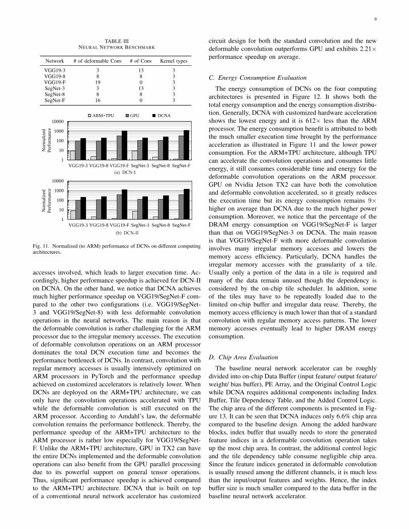
The performance of the DCN execution on the differentcomputing architectures is normalized to that on an ARMprocessor. As shown in Figure 11, DCNA achieves 515× and621× higher performance on DCN-I and DCN-II respectivelyon average compared to a general ARM processor. DCN-IIrequires more sampling locations in deformable convolutionoperations of DCNs, so it has more computation and random

9

TABLE IIINEURAL NETWORK BENCHMARK

Network # of deformable Conv # of Conv Kernel types

VGG19-3 3 13 3VGG19-8 8 8 3VGG19-F 19 0 3SegNet-3 3 13 3SegNet-8 8 8 3SegNet-F 16 0 3

1

10

100

1000

10000

ANET NIN FRCNN VGG16 VGG19 SEGNET

No

rmal

ized

Per

form

ance

1

10

100

1000

10000

ANET NIN FRCNN VGG16 VGG19 SEGNET

No

rmal

ized

Per

form

ance

ARM+TPU GPU DCNA

1

10

100

1000

10000

VGG19-3 VGG19-8 VGG19-F SegNet-3 SegNet-8 SegNet-F

No

rmal

ized

Per

form

ance

1

10

100

1000

10000


No

rmal

ized

Per

form

ance

Fig. 11. Normalized (to ARM) performance of DCNs on different computingarchitectures.

accesses involved, which leads to larger execution time. Ac-cordingly, higher performance speedup is achieved for DCN-IIon DCNA. On the other hand, we notice that DCNA achievesmuch higher performance speedup on VGG19/SegNet-F com-pared to the other two configurations (i.e. VGG19/SegNet-3 and VGG19/SegNet-8) with less deformable convolutionoperations in the neural networks. The main reason is thatthe deformable convolution is rather challenging for the ARMprocessor due to the irregular memory accesses. The executionof deformable convolution operations on an ARM processordominates the total DCN execution time and becomes theperformance bottleneck of DCNs. In contrast, convolution withregular memory accesses is usually intensively optimized onARM processors in PyTorch and the performance speedupachieved on customized accelerators is relatively lower. WhenDCNs are deployed on the ARM+TPU architecture, we canonly have the convolution operations accelerated with TPUwhile the deformable convolution is still executed on theARM processor. According to Amdahl’s law, the deformableconvolution remains the performance bottleneck. Thereby, theperformance speedup of the ARM+TPU architecture to theARM processor is rather low especially for VGG19/SegNet-F. Unlike the ARM+TPU architecture, GPU in TX2 can havethe entire DCNs implemented and the deformable convolutionoperations can also benefit from the GPU parallel processingdue to its powerful support on general tensor operations.Thus, significant performance speedup is achieved comparedto the ARM+TPU architecture. DCNA that is built on topof a conventional neural network accelerator has customized

circuit design for both the standard convolution and the newdeformable convolution outperforms GPU and exhibits 2.21×performance speedup on average.

C. Energy Consumption Evaluation

The energy consumption of DCNs on the four computingarchitectures is presented in Figure 12. It shows both thetotal energy consumption and the energy consumption distribu-tion. Generally, DCNA with customized hardware accelerationshows the lowest energy and it is 612× less than the ARMprocessor. The energy consumption benefit is attributed to boththe much smaller execution time brought by the performanceacceleration as illustrated in Figure 11 and the lower powerconsumption. For the ARM+TPU architecture, although TPUcan accelerate the convolution operations and consumes littleenergy, it still consumes considerable time and energy for thedeformable convolution operations on the ARM processor.GPU on Nvidia Jetson TX2 can have both the convolutionand deformable convolution accelerated, so it greatly reducesthe execution time but its energy consumption remains 9×higher on average than DCNA due to the much higher powerconsumption. Moreover, we notice that the percentage of theDRAM energy consumption on VGG19/SegNet-F is largerthan that on VGG19/SegNet-3 on DCNA. The main reasonis that VGG19/SegNet-F with more deformable convolutioninvolves many irregular memory accesses and lowers thememory access efficiency. Particularly, DCNA handles theirregular memory accesses with the granularity of a tile.Usually only a portion of the data in a tile is required andmany of the data remain unused though the dependency isconsidered by the on-chip tile scheduler. In addition, someof the tiles may have to be repeatedly loaded due to thelimited on-chip buffer and irregular data reuse. Thereby, thememory access efficiency is much lower than that of a standardconvolution with regular memory access patterns. The lowermemory accesses eventually lead to higher DRAM energyconsumption.

D. Chip Area Evaluation

The baseline neural network accelerator can be roughlydivided into on-chip Data Buffer (input feature/ output feature/weight/ bias buffer), PE Array, and the Original Control Logicwhile DCNA requires additional components including IndexBuffer, Tile Dependency Table, and the Added Control Logic.The chip area of the different components is presented in Fig-ure 13. It can be seen that DCNA induces only 6.6% chip areacompared to the baseline design. Among the added hardwareblocks, index buffer that usually needs to store the generatedfeature indices in a deformable convolution operation takesup the most chip area. In contrast, the additional control logicand the tile dependency table consume negligible chip area.Since the feature indices generated in deformable convolutionis usually reused among the different channels, it is much lessthan the input/output features and weights. Hence, the indexbuffer size is much smaller compared to the data buffer in thebaseline neural network accelerator.

10

0.01

0.1

1

10

100

1000

0%

20%

40%

60%

80%

100%

AR

M

AR

M+

TP

U

GP

U

DC

NA

AR

M

AR

M+

TP

U

GP

U

DC

NA

AR

M

AR

M+

TP

U

GP

U

DC

NA

AR

M

AR

M+

TP

U

GP

U

DC

NA

AR

M

AR

M+

TP

U

GP

U

DC

NA

AR

M

AR

M+

TP

U

GP

U

DC

NA

VGG19-3 VGG19-8 VGG19-F SegNet-3 SegNet-8 SegNet-FE

ner

gy

Co

nsu

mp

tio

n (

J)

0.01

0.1

1

10

100

1000

0%

20%

40%

60%

80%

100%

AR

M

AR

M+

TP

U

GP

U

DC

NA

AR

M

AR

M+

TP

U

GP

U

DC

NA

AR

M

AR

M+

TP

U

GP

U

DC

NA

AR

M

AR

M+

TP

U

GP

U

DC

NA

AR

M

AR

M+

TP

U

GP

U

DC

NA

AR

M

AR

M+

TP

U

GP

U

DC

NA


En

erg

y C

on

sum

pti

on

(J)

CPU DRAM GPU/TPU/DCNA Total Energy

Fig. 12. Energy consumption of DCNs on four computing architectures

0

1

2

3

4

5

6

7

8

Baseline DCNA

Are

a (m

m²)

Data Buffer PE ArrayOriginal Control Logic Index BufferAdded Control Logic Tile Status Table

0 1 2 3 4 5 6

Baseline

DCNA

Area (mm²)

Data Buffer PE Array Original Control Logic

Index Buffer Added Control Logic Tile Status Table

Fig. 13. Chip area of the baseline neural network accelerator and DCNA

E. Optimization Evaluation

Tile Scheduling: To evaluate the influence of the proposedtile scheduling on the DCN performance, we compare it witha naive implementation without bit vector based dependencytracking (W/O bit vector) and an implementation with bitvector based tracking but without tile scheduling (W/ bit vector+ W/O scheduling). The naive implementation executes theoutput features sequentially and loads all the dependent inputtiles as needed due to the lack of the overall dependencyinformation. The implementation with bit vector based track-ing but without tile scheduling sequentially executes all theoutput tiles, but it loads the dependent input tiles of the entireoutput tile rather than a single output feature based on thecorresponding TDT. The loaded input tiles will also be used forthe calculation of all the features in the output tile such that theloaded tiles can be reused as much as possible. The proposedimplementation has both the bit vector based tracking andtile scheduling considered (W/ bit vector + W/ scheduling). Itoptimizes the ordering of both the output tile execution and theinput tile loading for more efficient data reuse. The comparisonis shown in Figure 14. It can be seen that VGG19/SegNet-F with all the convolution layers replaced with deformableconvolution benefits most from the tile-based dependencytracking and scheduling. In contrast, VGG19/SegNet-8 haveonly three small convolution layers replaced with the de-

tpu

+ar

m

TX

2

AS

IC

tpu

+ar

m

TX

2

AS

IC

tpu

+ar

m

TX

2

AS

IC

tpu

+ar

m

TX

2

AS

IC

tpu

+ar

m

TX

2

AS

IC

tpu

+ar

m

TX

2

AS

IC

ANET NIN FRCNN VGG16 VGG19 SIGNET

0.005

0.01

0.015

0.02

0.142

0.2723 0.26712 0.25195 0.24817 0.24645 0.24166

tpu+

arm

TX

2

AS

IC

tpu+

arm

TX

2

AS

IC

tpu+

arm

TX

2

AS

IC

tpu+

arm

TX

2

AS

IC

tpu+

arm

TX

2

AS

IC

tpu+

arm

TX

2

AS

IC


0.005

0.01

0.0150.02

0

0

0.26576 0.25634 0.24587 0.22011 0.21947 0.20334

CPU DDR GPU accelerator

No

rmali

zed

En

erg

y

(lo

wer

is

bet

ter)

No

rmali

zed

En

erg

y

(lo

wer

is

bet

ter)

(a) POI-DCNN

(b) F-DCNN

0.125

tpu+

arm

TX

2

AS

IC

tpu+

arm

TX

2

AS

IC

tpu+

arm

TX

2

AS

IC

tpu+

arm

TX

2

AS

IC

tpu+

arm

TX

2

AS

IC

tpu+

arm

TX

2

AS

IC


0.005

0.01

0.015

0.02

0

0.26576 0.25634 0.24587 0.22011 0.21947 0.20334

CPU DDR GPU accelerator

No

rmal

ized

En

erg

y

(lo

wer

is

bet

ter)

(a) POI-DCNN

0.125


0

0.5

1

1.5

2

2.5

Norm

aliz

ed

Perf

orm

ance

12.9x16.5x 23.6x

32.1x


0

0.5

1

1.5

2

2.5

Norm

aliz

ed

Perf

orm

ance

3.1x4.6x 10.4x

13.2x

(b) DCN-II

(a) DCN-I

W/O bit vector W/ bit vector +W/O schedulIng W/ bit vector +W/ scheduling

Fig. 14. Influence of tile scheduling on the DCN performance.

formable convolution exhibits marginal performance speedup.It is mainly caused by two reasons. First, the computation ofthe deformable convolution operations takes up only a smallportion of the entire neural network computation, there islittle space left for the performance improvement. Second,the sizes of the deformable convolution operations are smalland the data including the input features, the weights, and theoutput features can be mostly fully buffered. Hence, the tilescan be reused without any scheduling and the proposed tilescheduling shows no performance improvement in this case.The performance improvement on DCN-I and DCN-II alsodiffers. This is mainly caused by the fact that DCN-II involvesmore random sampling and thus benefits more from the DCNAacceleration.

On top of the performance improvement, we also evaluatethe influence of the tile scheduling on the energy consumptionof the DCN execution. The experiment result is shown inFigure 15. Again, it can be seen that VGG19/SegNet-F withmost deformable convolution operations benefits most andshows the least energy consumption while VGG19/SegNet-3 with small deformable convolution operations has littleoptimization space for the tile scheduling. Generally, theenergy reduction is mainly attributed to both the reducedexecution time according to Figure 14 and the lower powerconsumption brought by the reduced memory accesses. Asthe performance improvement is already discussed in priorsubsection, we mainly investigate the memory access reductionin this subsection. The total memory accesses issued byDCNA during the DCN processing is shown in Figure 16.By comparing the implementation without bit vector baseddependency tracking and the implementation with bit vectorbut no scheduling, we observe that the bit vector based tiledependency tracking removes substantial memory accesses. Itis mainly achieved by avoiding repeatedly loading the sameinput tiles required by the calculation of different outputfeatures in the same output tile. The scheduling further reducesthe memory accesses by inspecting the input tile reuse amongthe different output tiles according to the tile dependencytable. The experiment shows that the proposed scheduling

11

0

0.2

0.4

0.6

0.8

1

VGG19-3 VGG19-8VGG19-F SegNet-3 SegNet-8 SegNet-F

Norm

aliz

ed E

ner

gy

0

0.2

0.4

0.6

0.8

1

VGG19-3VGG19-8VGG19-F SegNet-3 SegNet-8 SegNet-F

Norm

aliz

ed E

ner

gy

(a) DCN-I

(b) DCN-II

W/O bit vector W/ bit vector +W/O scheduling W/ bit vector +W/ scheduling

Fig. 15. Influence of tile scheduling on the DCN energy consumption.

0

0.2

0.4

0.6

0.8

1


Norm

aliz

ed M

emm

ory

Acc

ess

Num

ber

0

0.2

0.4

0.6

0.8

1


Norm

aliz

ed M

emm

ory

Acc

ess

Num

ber

0%

20%

40%

60%

80%

100%

Layer3 Layer4 Layer5

0%

20%

40%

60%

80%

100%

Layer3 Layer4 Layer5

Without bitmap Bitmap-based sequential loading strategy Bitmap-based scheduling loading strategy

(a) DCN-I

(b) DCN-II

W/O bit vector W/ bit vector +W/O scheduling W/ bit vector +W/ scheduling

Fig. 16. Influence of tile scheduling on the number of DCN memory accesses.

reduces the memory accesses by 40.7% on VGG19/SegNet-F on average compared to the implementation with only bitvector based dependency tracking.

Tile Sizing: Tile size is an important design parameter andit determines the granularity of the tile dependency trackingand scheduling. Since most of the memory access latency inDCNA can be overlapped by the computing latency, tile sizemainly affects the memory access efficiency and the DRAMenergy consumption eventually, and has little influence on theperformance. We take VGG19/SegNet-F with most deformableconvolution operations as an example and analyzed the DRAMenergy consumption under different tile sizes. The experimentresult is shown in Figure 17. It can be seen that the DCNprocessing with smaller tile size benefits most from DCNAand consumes the least DRAM energy. The main reason isthat smaller tile size allows more efficient tile dependencytracking and scheduling. Thus, the on-chip buffer utilizationand DRAM memory access efficiency can be improved. Incontrast, when the tile size is large, the dependent inputfeatures of each output tile can spread across all the input tiles.In this case, all the input tiles have to be repeatedly loaded for

0

0.2

0.4

0.6

0.8

1

9 16 25 64No

rmal

ized

DR

AM

En

erg

y

Tile size

0

0.2

0.4

0.6

0.8

1

9 16 25 64

No

rmal

ized

DR

AM

En

erg

y

Tile size

(a) DCN-I

VGG19-F SegNet-F

(b) DCN-II

Fig. 17. Normalized DRAM energy consumption under different tile sizes.

each output tile calculation, leaving little optimization spacefor the proposed tile dependency tracking and scheduling.

Layer Fusion: In order to reduce the intermediate datatransmission to and from DRAM, we propose to fuse theprocessing stages in each deformable convolution operation.The influence of the layer fusion on the energy consumptionis shown in Figure 18. It can be seen that the fusion reduces theenergy consumption by more than 20% on VGG19/SegNet-Fwith DCN-II structure. The main reason is that the memoryaccess time in the two DCNs cannot be fully overlapped by thecomputation time due to the involved large deformable convo-lution operations and the fusion that avoids large intermediatedata transmission improves the DCN performance other thanthe memory access efficiency. Unlike VGG19/SegNet-F, thedeformable convolution operations in the rest scenarios arerelatively small and the fusion only reduces the memoryaccesses while the performance has little improvement. As theDRAM energy consumption takes up only around 20% of theentire DCN energy consumption according to Figure 12, theenergy reduction brought by the memory reduction is limited.Particularly, for VGG19/SegNet-3, the entire intermediate datacan be mostly fully buffered and there is even little memoryaccess optimization space left for the fusion. Thereby, thefusion shows little energy reduction.

VI. CONCLUSION

DCNs that have been demonstrated to be effective in manypractical scenarios with image geometric or photometric vari-ations include new deformable convolution operations otherthan the conventional neural network operations. The de-formable convolution operations that require random samplingover the entire input feature maps incur considerable irregularmemory accesses and bilinear interpolation (BLI) operations,which that can not be fitted to the existing neural network ac-celerator architecture. In this work, we revisit the conventionalneural network architecture by introducing a runtime tile-based data dependency tracking and scheduling mechanism

12

0

0.2

0.4

0.6

0.8

1


Norm

aliz

ed E

ner

gy

0

0.2

0.4

0.6

0.8

1


No

rmal

ized

En

erg

y

0%

20%

40%

60%

80%

100%

Layer1 Layer2 Layer3 Layer4

Without Fusing With Fusing

0%

20%

40%

60%

80%

100%

Layer1 Layer2 Layer3 Layer4

(a) POI-DCNN (b) F-DCNN

(a) DCN-I

W/O Fusing W/ Fusing

(b) DCN-II

Fig. 18. Influence of layer fusion on the DCN energy consumption.

to address the irregular memory accesses and optimize thedata reuse in DCNs. At the same time, we reorganize the BLIoperations to fit them to the 2D computing array for parallelprocessing. Finally, we also fuse the different processing stagesin each deformable convolution operation to enable on-chipdata reuse and reduce the intermediate data transmission viaDRAM. According to our experiments on representative neuralnetworks with different deformable convolution configura-tions, the proposed DCNA that supports both the convolutionand deformable convolution achieves 45×-546× performancespeedup over the ARM+TPU architecture that relies on theARM processor to handle the deformable convolution. Whencompared to GPU that can execute the entire DCNs, DCNAshows 3× performance speedup and 18.6× energy reduction.

REFERENCES

[1] J. Dai, H. Qi, Y. Xiong, Y. Li, G. Zhang, H. Hu, and Y. Wei, “Deformableconvolutional networks,” in Proceedings of the IEEE internationalconference on computer vision, 2017, pp. 764–773.

[2] Z. Cao, X. Li, and L. Zhao, “Object detection in vhr image usingtransfer learning with deformable convolution,” in IGARSS 2019-2019IEEE International Geoscience and Remote Sensing Symposium. IEEE,2019, pp. 326–329.

[3] C. Zhang and J. Kim, “Object Detection With Location-Aware De-formable Convolution and Backward Attention Filtering,” in 2019IEEE/CVF Conference on Computer Vision and Pattern Recognition(CVPR), 2019, pp. 9444–9453.

[4] D. Zhang, L. Li, Z. Zhu, S. Jin, W. Gao, and C. Li, “Object DetectionAlgorithm Based on Deformable Convolutional Networks for Underwa-ter Images,” in 2019 2nd China Symposium on Cognitive Computingand Hybrid Intelligence (CCHI), 2019, pp. 274–279.

[5] L. Deng, M. Yang, H. Li, T. Li, B. Hu, and C. Wang, “Restricteddeformable convolution-based road scene semantic segmentation usingsurround view cameras,” IEEE Transactions on Intelligent Transporta-tion Systems, 2019.

[6] L.-C. Chen, Y. Zhu, G. Papandreou, F. Schroff, and H. Adam, “Encoder-decoder with atrous separable convolution for semantic image segmen-tation,” in Proceedings of the European conference on computer vision(ECCV), 2018, pp. 801–818.

[7] Y. Xiong, R. Liao, H. Zhao, R. Hu, M. Bai, E. Yumer, and R. Urta-sun, “UPSNet: A Unified Panoptic Segmentation Network,” in 2019IEEE/CVF Conference on Computer Vision and Pattern Recognition(CVPR), 2019, pp. 8810–8818.

[8] Y. Diao, J. Chen, and Y. Qian, “Multi-Label Remote Sensing Im-age Classification with Deformable Convolutions and Graph NeuralNetworks,” in IGARSS 2020-2020 IEEE International Geoscience andRemote Sensing Symposium. IEEE, 2020, pp. 521–524.

[9] N. G. M. Lu, “DeformSketchNet: Deformable Convolutional Networksfor Sketch Classification.”

[10] S. C. Lai, H. K. Tan, and P. Y. Lau, “3D Deformable Convolution forAction Classification in Videos,” in International Workshop on AdvancedImaging Technology (IWAIT) 2021, vol. 11766. International Societyfor Optics and Photonics, 2021, p. 117660R.

[11] X. Sun, B. Xiao, F. Wei, S. Liang, and Y. Wei, “Integral Human PoseRegression,” in Proceedings of the European Conference on ComputerVision (ECCV), 2018, pp. 529–545.

[12] J. Weng, M. Liu, X. Jiang, and J. Yuan, “Deformable pose traversalconvolution for 3d action and gesture recognition,” in Proceedings ofthe European Conference on Computer Vision (ECCV), 2018, pp. 136–152.

[13] G. Bertasius, L. Torresani, and J. Shi, “Object Detection in Video withSpatiotemporal Sampling Networks,” in Proceedings of the EuropeanConference on Computer Vision (ECCV), 2018, pp. 331–346.

[14] K.-N. C. Mac, D. Joshi, R. A. Yeh, J. Xiong, R. R. Feris, and M. N. Do,“Locally-consistent deformable convolution networks for fine-grainedaction detection,” arXiv preprint arXiv:1811.08815, 2018.

[15] Z. Li, H. Pan, Y. Zhu, and A. K. Qin, “PGD-UNet: A Position-GuidedDeformable Network for Simultaneous Segmentation of Organs andTumors,” in 2020 International Joint Conference on Neural Networks(IJCNN), 2020, pp. 1–8.

[16] M. Pominova, E. Kondrateva, M. Sharaev, A. Bernstein, S. Pavlov, andE. Burnaev, “3D Deformable Convolutions for MRI Classification,” in2019 18th IEEE International Conference On Machine Learning AndApplications (ICMLA), 2019, pp. 1710–1716.

[17] G. Y. Huang Q, Wang D et al., “Algorithm-hardware Co-design forDeformable Convolution,” 2020, p. arXiv:2002.08357.

[18] S. Ahn, J.-W. Chang, and S.-J. Kang, “An Efficient Accelerator DesignMethodology For Deformable Convolutional Networks,” in 2020 IEEEInternational Conference on Image Processing (ICIP), 2020, pp. 3075–3079.

[19] Y.-H. Chen, J. Emer, and V. Sze, “Eyeriss: A spatial architecturefor energy-efficient dataflow for convolutional neural networks,” in2016 ACM/IEEE 43rd Annual International Symposium on ComputerArchitecture (ISCA). IEEE, 2016, pp. 367–379.

[20] J. Albericio, P. Judd, T. Hetherington, T. Aamodt, N. E. Jerger, andA. Moshovos, “Cnvlutin: Ineffectual-Neuron-Free Deep Neural NetworkComputing,” ACM SIGARCH Computer Architecture News, vol. 44,no. 3, pp. 1–13, 2016.

[21] M. Bromberger, P. Bastian, J.-P. Bergeest, C. Conrad, V. Heuveline,K. Rohr, and W. Karl, “FPGA-accelerated Richardson-Lucy Deconvolu-tion for 3D Image Data,” in 2016 IEEE 13th International Symposiumon Biomedical Imaging (ISBI). IEEE, 2016, pp. 132–135.

[22] Y. Wang, J. Xu, Y. Han, H. Li, and X. Li, “DeepBurning: AutomaticGeneration of FPGA-based Learning Accelerators for the Neural Net-work Family,” in Proceedings of the 53rd Annual Design AutomationConference. ACM, 2016, p. 110.

[23] C. Zhang, G. Sun, Z. Fang, P. Zhou, P. Pan, and J. Cong, “Caffeine:Towards Uniformed Representation and Acceleration for Deep Convolu-tional Neural Networks,” IEEE Transactions on Computer-Aided Designof Integrated Circuits and Systems, 2018.

[24] D. Xu, Q. Wang, C. Liu, C. Chu, Y. Wang, H. Li, X. Li, and K.-T.Cheng, “Hyca: A hybrid computing architecture for fault tolerant deeplearning,” arXiv preprint arXiv:2106.04772, 2021.

[25] D. Xu, C. Chu, Q. Wang, C. Liu, Y. Wang, L. Zhang, H. Liang, andK.-T. Cheng, “A hybrid computing architecture for fault-tolerant deeplearning accelerators,” in 2020 IEEE 38th International Conference onComputer Design (ICCD). IEEE, 2020, pp. 478–485.

[26] D. Xu, K. Tu, Y. Wang, C. Liu, B. He, and H. Li, “FCN-Engine:Accelerating Deconvolutional Layers in Classic CNN Processors,” inProceedings of the International Conference on Computer-Aided Design.ACM, 2018, p. 22.

[27] A. Yazdanbakhsh, K. Samadi, N. S. Kim, and H. Esmaeilzadeh, “Ganax:A Unified MIMD-SIMD Acceleration for Generative Adversarial Net-works,” in Proceedings of the 45th Annual International Symposium onComputer Architecture. IEEE Press, 2018, pp. 650–661.

[28] J. Yan, S. Yin, F. Tu, L. Liu, and S. Wei, “Gna: Reconfigurableand efficient architecture for generative network acceleration,” IEEETransactions on Computer-Aided Design of Integrated Circuits andSystems, vol. 37, no. 11, pp. 2519–2529, 2018.

[29] X. Zhang, S. Das, O. Neopane, and K. Kreutz-Delgado, “A designmethodology for efficient implementation of deconvolutional neuralnetworks on an fpga,” arXiv preprint arXiv:1705.02583, 2017.

[30] K. Hegde, R. Agrawal, Y. Yao, and C. W. Fletcher, “Morph: FlexibleAcceleration for 3D CNN-based Video Understanding,” in 2018 51st

13

Annual IEEE/ACM International Symposium on Microarchitecture (MI-CRO). IEEE, 2018, pp. 933–946.

[31] H. Wang, M. Shao, Y. Liu, and W. Zhao, “Enhanced efficiency 3dconvolution based on optimal fpga accelerator,” IEEE Access, vol. 5,pp. 6909–6916, 2017.

[32] H. Fan, H.-C. Ng, S. Liu, Z. Que, X. Niu, and W. Luk, “Reconfigurableacceleration of 3d-cnns for human action recognition with block floating-point representation,” in 2018 28th International Conference on FieldProgrammable Logic and Applications (FPL). IEEE, 2018, pp. 287–2877.

[33] C. Chu, F. Chen, D. Xu, and Y. Wang, “RECOIN: A Low-PowerProcessing-in-ReRAM Architecture for Deformable Convolution,” inGLSVLSI ’21: Great Lakes Symposium on VLSI 2021, 2021.

[34] M. Alwani, H. Chen, M. Ferdman, and P. Milder, “Fused-Layer CNN

Accelerators,” in 2016 49th Annual IEEE/ACM International Symposiumon Microarchitecture (MICRO). IEEE, 2016, pp. 1–12.

[35] A. Samajdar, Y. Zhu, P. Whatmough, M. Mattina, and T. Krishna,“SCALE-Sim: Systolic CNN Accelerator Simulator,” arXiv preprintarXiv:1811.02883, 2018.

[36] https://www.micron.com/support/tools-and-utilities/power-calc.[37] K. Simonyan and A. Zisserman, “Very Deep Convolutional Networks

for Large-Scale Image Recognition,” arXiv preprint arXiv:1409.1556,2014.

[38] V. Badrinarayanan, A. Kendall, and R. Cipolla, “SegNet: A DeepConvolutional Encoder-Decoder Architecture for Image Segmentation,”IEEE transactions on pattern analysis and machine intelligence, vol. 39,no. 12, pp. 2481–2495, 2017.

https://www.micron.com/support/tools-and-utilities/power-calc

Energy-Efﬁcient Accelerator Design for Deformable ...

Documents

Transcript of Energy-Efﬁcient Accelerator Design for Deformable ...