Energy Decay of Vortices in Viscous Fluids: an Applied ...

Energy Decay of Vortices in Viscous Fluids: an

Applied Mathematics View

Jan Nordström and Björn Lönn

Linköping University Post Print

N.B.: When citing this work, cite the original article.

Original Publication:

Jan Nordström and Björn Lönn, Energy Decay of Vortices in Viscous Fluids: an Applied

Mathematics View, 2012, Journal of Fluid Mechanics.

http://dx.doi.org/10.1017/jfm.2012.351

Copyright: Cambridge University Press (CUP)

http://www.cambridge.org/uk/

Postprint available at: Linköping University Electronic Press

http://urn.kb.se/resolve?urn=urn:nbn:se:liu:diva-80799

http://dx.doi.org/10.1017/jfm.2012.351

http://www.cambridge.org/uk/

http://urn.kb.se/resolve?urn=urn:nbn:se:liu:diva-80799

Under consideration for publication in J. Fluid Mech. 1

Energy Decay of Vortices in Viscous Fluids:an Applied Mathematics View

JAN NORDSTROM1†AND BJ ORN LONN 2

1Department of Mathematics, Linkoping University, SE-581 83 Linkoping, Sweden2Department of Information Technology, Uppsala University, SE-75105 Uppsala, Sweden

(Received ?; revised ?; accepted ?. - To be entered by editorial office)

The energy decay of vortices in viscous fluids governed by the compressible Navier-Stokes equations is investigated. It is shown that the main reason for the slow decay isthat zero eigenvalues exist in the matrix related to the dissipative terms. The theoreticalanalysis is purely mathematical and based on the energy method. To check the validity ofthe theoretical result in practice, numerical solutions to the Navier-Stokes equations arecomputed using a stable high order finite difference method. The numerical computationscorroborate the theoretical conclusion.

Key words:

1. IntroductionVortices are common flow features in aeronautical applications. The topic of this paper,

the slow energy decay, causes problems when wingtip vortices remain on the runway fora long time, see Proctor (1998), Kantha (2010), Gerz et al. (2002), Breitsamter (2011),Spalart (1998). Vortices are also important when explaining several flow phenomena. Thelift generated by wings is investigated in Chen et al. (2010), Rossow (1999), Yen (2011).It is concluded that effects from leading edge vortices can be used to increase lift.

Vortices are frequently present in nature and also influence the environment. Thepresence of von Karman vortices in the trailing wind of islands can have effects on thelocal climate as well as the sea life, see Beggs et al. (2004), Ponta (2010), Holzapfel et al.(2003). Their effect on fish, bird and insect behavior is studied in Wu (2011), Kim & Kim(2011), Liu et al. (2009). Vortices are also needed when modeling the general circulationof the ocean as seen in Holland (1978), Zhang et al. (2011), Winter & Bourqui (2011),Koszalka et al. (2011). Other effects include emissions from air traffic Gerz & Holzapfel(1999) and influence on the efficiency of turbine parks Magnusson & Smedman (1999).

It is well known that vortices do not decay in inviscid flows governed by the Euler equa-tions. It is quite straightforward to construct exact solutions that advect with a constantbackground velocity, see Anderson (1991), McCormack & Crane (1973), Erlebacher et al.(1997), Davoudzadeh et al. (1995). Less well known is why this slow energy decay seemto persist also in viscous flows governed by the Navier-Stokes equations. This phenomenahas been thoroughly investigated and many theories of what phenomena are importantand why the decay is slow exist, see for example Sarpkaya (1998), Matthaeus et al. (1991),Gustavsson (1991), Greene (1986), Balmforth et al. (2001), Greene (1986), Zhou et al.(1999), Wallin & Girimaji (2000), Pullin & Saffman (1998), Winckelmans et al. (2006),

† Email address for correspondence: [email protected]

2 J. Nordstrom and B. Lonn

Kundu & Cohen (2001). Related but more fundamental theoretical questions like stabil-ity and existence of solutions for long times were studied in Hoff & Zumbrum (1995),Hagstrom & Lorenz (1995) and Hagstrom & Lorenz (2002).

Most of the previous investigations and theories are based on observations of measuredor computed data and a subsequent analysis. We will take a different approach and relyon mathematics only. This will eliminate potential error sources when producing data,make the analysis transparent to the reader and hence enable the reader to follow andcheck the whole procedure. Only afterwards, when the main theoretical conclusion hasbeen reached, and the suggested decay scenario has been formulated will the implicationsof the theory be tested using results from numerical calculations.

We begin by observing that vortices exist for all ranges of Reynolds numbers (with theexception of Stokes flow) including inviscid flows. This indicate that the size of the viscousterms is not of fundamental importance. Hence, it is relevant to analyse a simple laminarflow case, without considering complicated additional phenomena such as turbulence.We will analyse the energy decay of small scale disturbances by applying the standardtool in applied mathematics/numerical analysis, namely the energy-method (see Kreiss& Lorenz (1989) and Gustafsson et al. (1995) and the numerous references therein). Inparticular we will investigate the viscous terms and their role in the energy dissipation.

2. AnalysisConsider the flow situation when small disturbances are imposed on a constant back-

ground state. This could be a model of the situation right after the passing of an aircraftin free space. This problem setup also naturally allows for the linearized analysis belowwhere we neglect quadratic terms and investigate the decay of small scale disturbances.

The dependent variables are the density ρ, the velocities in each direction u, v, w andthe temperature T . The tilde sign signifies the presence of dimensions. We write theequations in non-dimensional form using the free stream density ρ∞, the free streamvelocity U∞ and the free stream temperature T∞. The shear and second viscosity co-efficients µ, λ as well as the coefficient of heat conduction κ are non-dimensionalizedwith the free stream viscosity µ∞. The pressure in non-dimensional form becomes:p = p/(ρ∞U2

∞) = ρT/(γM2∞). Also used are

M2∞ =

U2∞

γRT∞, P r =

µ∞Cpκ∞

, Re =ρ∞U∞L

µ∞, γ =

CpCv

, ϕ =γκ

Pr(2.1)

where L is a length scale and M , Pr, Re = 1/ε and γ are the Mach-, Prandtl-, Reynoldsnumber and ratio of specific heats respectively. The time scale is L/U∞.

2.1. The energy methodThe linearized dimensionless compressible Navier-Stokes equations can formally be writ-ten

∂V

∂t+ A

∂V

∂x+ B

∂V

∂y+ C

∂V

∂z=ε

ρ[(D11

∂V

∂x+ D12

∂V

∂y+ D13

∂V

∂z)x +

+(D21∂V

∂x+ D22

∂V

∂y+ D23

∂V

∂z)y + (D31

∂V

∂x+ D32

∂V

∂y+ D33

∂V

∂z)z]. (2.2)

In (2.2), V = (ρ, u, v, w, T )T is the disturbance and the constant state around which welinearize is denoted by an overbar. The matrices related to the hyperbolic terms in (2.2)must be symmetric for the energy method to be applicable Nordstrom & Svard (2005).

Energy Decay of Vortices in Viscous Fluids 3

In Abarbanel & Gottlieb (1981) it is shown that the symmetrization can be done usinga single matrix S. We choose the symmetrizer

S−1 = diag

[c2√γ, ρc, ρc, ρc,

ρ√γ(γ − 1)M4

∞

], (2.3)

where c is the speed of sound at reference state.Remark: Abarbanel & Gottlieb (1981) showed that the three-dimensional compress-

ible Navier-Stokes equations with 12 matrices involved (see (2.2)), can be symmetrizedby a single matrix (symmetrizer). This remarkable fact was complemented by the obser-vation that there are at least two different symmetrizers, based on either the hyperbolicor the parabolic terms. The symmetrizer (2.3) is related to the parabolic terms.

The similarity transform is applied by multiplying (2.2) from the left with S−1. Afterapplying the symmetrizer we obtain

A =

u c/

√γ 0 0 0

c/√γ u 0 0 c

√γ−1γ

0 0 u 0 00 0 0 u 0

0 c√

γ−1γ 0 0 u

D11 =

0 0 0 0 00 2µ+ λ 0 0 00 0 µ 0 00 0 0 µ 00 0 0 0 ϕ

(2.4)

B =

v 0 c/

√γ 0 0

0 v 0 0 0

c/√γ 0 v 0 c

√γ−1γ

0 0 0 v 0

0 0 c√

γ−1γ 0 v

D22 =

0 0 0 0 00 µ 0 0 00 0 2µ+ λ 0 00 0 0 µ 00 0 0 0 ϕ

(2.5)

C =

w 0 0 c/

√γ 0

0 w 0 0 00 0 w 0 0

c/√γ 0 0 w c

√γ−1γ

0 0 0 c√

γ−1γ w

D33 =

0 0 0 0 00 µ 0 0 00 0 µ 0 00 0 0 2µ+ λ 00 0 0 0 ϕ

(2.6)

D12 = DT21 =

0 0 0 0 00 0 λ 0 00 µ 0 0 00 0 0 0 00 0 0 0 0

D13 = DT31 =

0 0 0 0 00 0 0 λ 00 0 0 0 00 µ 0 0 00 0 0 0 0

(2.7)

D23 = DT32 =

0 0 0 0 00 0 0 0 00 0 0 λ 00 0 µ 0 00 0 0 0 0

V =

c2√γ ρ

ρcuρcvρcwρ√

γ(γ−1)M4∞T

(2.8)

where V T = (S−1V )T , A = S−1AS, B = S−1BS, C = S−1CS and the Dij ’s are


unchanged. The matrices above are all given in Abarbanel & Gottlieb (1981) but we listthem here for completeness.

The energy method is applied by multiplying the symmetrized dimensionless Navier-Stokes equations with V T and integrating over the domain Ω. Let the energy norm bedefined as ||V ||2 =

∫ΩV T V dxdydz. By using Gauss’ theorem and integration by parts,

we obtain

||V ||2t +BT = −2(ε

ρ)∫

Ω

VxVyVz

T D11 D12 D13

D21 D22 D23

D31 D32 D33

VxVyVz

dxdydz, (2.9)

where

BT =∮∂Ω

V T [AV − 2( ερ )(D11Vx + D12Vy + D13Vz)]V T [BV − 2( ερ )(D21Vx + D22Vy + D23Vz)]V T [CV − 2( ερ )(D31Vx + D32Vy + D33Vz)]

· n ds. (2.10)

In (2.10), ds =√dx2 + dy2 + dz2 and n = (n1, n2, n3)T is the outward pointing unit

normal on the surface ∂Ω.In this paper we ignore the effect of far-field boundaries and consider the Cauchy

problem only. In particular, we focus on the volume term on the right-hand-side of (2.9)and neglect the boundary term BT. Let the block matrix consisting of the Dij matricesbe denoted by D. If D is positive semi-definite, (2.9) show that the energy decays.

Remark: Normally the relations (2.9) and (2.10) are used in order to determine bound-ary conditions that lead to well-posedness, see for example Gustafsson & Sundstrom(1978), Nordstrom (1995) and Nordstrom & Svard (2005). In that case the focus is onthe term BT.

Remark: If D would not be positive semi-definite, then (2.9) would show that theCauchy problem for the linearized Navier-Stokes equation is not well posed.

The first, sixth and 11th rows as well as the first, sixth and 11th columns of the 15x15matrix D have only zero elements, thus the matrix can be reduced to a 12x12 matrix.We refer to this matrix as D.

D =

2µ+ λ 0 0 0 0 λ 0 0 0 0 λ 00 µ 0 0 µ 0 0 0 0 0 0 00 0 µ 0 0 0 0 0 µ 0 0 00 0 0 ϕ 0 0 0 0 0 0 0 00 µ 0 0 µ 0 0 0 0 0 0 0λ 0 0 0 0 2µ+ λ 0 0 0 0 λ 00 0 0 0 0 0 µ 0 0 µ 0 00 0 0 0 0 0 0 ϕ 0 0 0 00 0 µ 0 0 0 0 0 µ 0 0 00 0 0 0 0 0 µ 0 0 µ 0 0λ 0 0 0 0 λ 0 0 0 0 2µ+ λ 00 0 0 0 0 0 0 0 0 0 0 ϕ

(2.11)

The eigenvalues of D are obtained by solving det(D − sI) = 0 for s which yield s =ϕ,ϕ, ϕ, 2µ, 2µ, 2µ, 0, 0, 0, 2µ, 2µ, 2µ + 3λ. The second law of thermodynamics, see White(1974), imply that 2µ + 3λ > 0 and hence all the eigenvalues are positive semi-definiteas required for a well posed problem.

To see how the velocity gradients and the eigenvalues are related, the eigenvectors


must be calculated. The orthonormal matrix with the eigenvectors as columns is

Q =

0 0 0 0 0 0 0 0 0√

16

1√2

1√3

0 0 0 1√2

0 0 1√2

0 0 0 0 00 0 0 0 1√

20 0 1√

20 0 0 0

1 0 0 0 0 0 0 0 0 0 0 00 0 0 1√

20 0 −1√

20 0 0 0 0

0 0 0 0 0 0 0 0 0 −√

46 0 1√

3

0 0 0 0 0 1√2

0 0 1√2

0 0 00 1 0 0 0 0 0 0 0 0 0 00 0 0 0 1√

20 0 −1√

20 0 0 0

0 0 0 0 0 1√2

0 0 −1√2

0 0 0

0 0 0 0 0 0 0 0 0√

16 − 1√

21√3

0 0 1 0 0 0 0 0 0 0 0 0

. (2.12)

We obtain D = QΛQT where Λ = diag(ϕ,ϕ, ϕ, 2µ, 2µ, 2µ, 0, 0, 0, 2µ, 2µ, 2µ + 3λ). Byinserting D (or the identical D) into (2.9) we obtain the final form of the energy decayrate

||V ||2t = −2(ε

ρ)∫D

QT Vx

VyVz

T Λ

QT Vx

VyVz

dxdydz , (2.13)

where

QT

VxVyVz

=

ρ√γ(γ−1)M4

∞Tx

ρ√γ(γ−1)M4

∞Ty

ρ√γ(γ−1)M4

∞Tz

1√2ρc[vx + uy]

1√2ρc[wx + uz]

1√2ρc[wy + vz]

1√2ρc[vx − uy]

1√2ρc[wx − uz]

1√2ρc[wy − vz]√

23 ρc[

12ux − vy + 1

2wz]1√2ρc[ux − wz]

1√3ρc[ux + vy + wz]

. (2.14)

2.2. Analysis of the energy decay rateThe relation (2.13) and (2.14) show the relation between eigenvalues and gradients. Thetemperature gradients are multiplied by the eigenvalue ϕ. The following three componentsconsist of terms related to the rotation of the velocity field in the xy-, xz- and yz planesand are each multiplied by 2µ. The most interesting fact is that the vorticity componentsin each plane are multiplied by a zero eigenvalue. The last term is the divergence andit is multiplied by the positive eigenvalue 2µ + 3λ. The two remaining terms consist ofcomponents related to the divergence ux + vy + wz and they are multiplied by 2µ.

Based on (2.13) and (2.14) we can now draw the two central conclusions of this paper:


• The vorticity terms are multiplied by zero eigenvalues.• The decay rate is proportional to the gradients squared.

These conclusions suggest that vortices will decay slowly because the main part of the en-ergy is concentrated in the vorticity components. They also indicate that flow structureswith gradients that are not in vorticity form will decay fast.

Remark: The velocity gradient can be decomposed into symmetric and antisymmetricparts (strain-rate and vorticity tensors). The eigenvalues associated with the vorticitytensor are zero while eigenvalues associated with the strain-rate tensor are non-zero. Theonly flow condition that has zero strain rate and non-zero vorticity is solid body rotation,which, according to the analysis, is the only flow that will be undamped. All other kindof vortical flows will be damped since it will contain some amount of strain rate.

Remark: The analysis above show that if all the energy reside in the vorticity compo-nents, there is no energy decay. However, the energy can be transferred to other modesand lead to decay. If the transfer is slow, the energy decay will be small. On the other handit is also possible to have an energy decay that halts due to the transfer of energy fromnon-vorticity modes into vorticity modes. It is not possible (although indications exist,see Hoff & Zumbrum (1995)) to analytically determine whether such a transfer exist andhow fast it is, but we will investigate this below by performing numerical calculations.

3. Numerical calculationsThe computations are done using a well tested and provable stable high order finite

difference scheme for the compressible Navier-Stokes equations. It uses summation-by-parts operators and imposes boundary and interface conditions weakly as described inCarpenter et al. (1999), Nordstrom & Carpenter (1999), Nordstrom & Carpenter (2001),Mattsson et al. (2004), Svard et al. (2007), Svard & Nordstrom (2008) and Nordstromet al. (2009). The code runs with 2,3,4 and 5th order global accuracy. The 3rd orderaccurate scheme with far field boundaries sufficiently far from the actual flow structurewas used.

3.1. The grids and order of accuracyThe grid used for calculations in two dimensions is each divided into 16 blocks. All blockshave an equal number of grid points. The grid used, for the displayed computations, is asquare with side length 20 and 257 points each in both the x and y directions. Hence themesh has ∆x = ∆y = 0.078. For calculations in three dimensions the grid is a cube withside length 20 and it has 129 points in each direction giving ∆x = ∆y = ∆z = 0.155.The 3rd order accurate scheme was evaluated in two dimensions using the 33-65-129, 65-129-257 and 129-257-513 point grids. The practical order of accuracy obtained was 1.71,2.18 and 2.40 respectively. The error level in L2 norm for the displayed 2D computationsis estimated to 3× 10−7.

3.2. Initial conditions in two dimensionsTo verify the analytical results, long time simulations with three different initial condi-tions have been investigated. The Reynolds numbers considered are Re = 10, 100 andRe = 1000. We stress here that the size of the Reynolds number is of no fundamentalimportance in this investigation. The zero eigenvalues are present for all Reynolds num-bers. We have compared the energy decay of a vortex, with the energy decay of whitenoise, and a specially constructed divergence free flow case. As initial values for all thesetwo dimensional calculations we used: the Mach number M=0.005, the radius r=1, thedensity and temperature are ρ∞ = 1, T∞ = 1.


x

y

-10 -5 0 5 10-10

-5

0

5

10

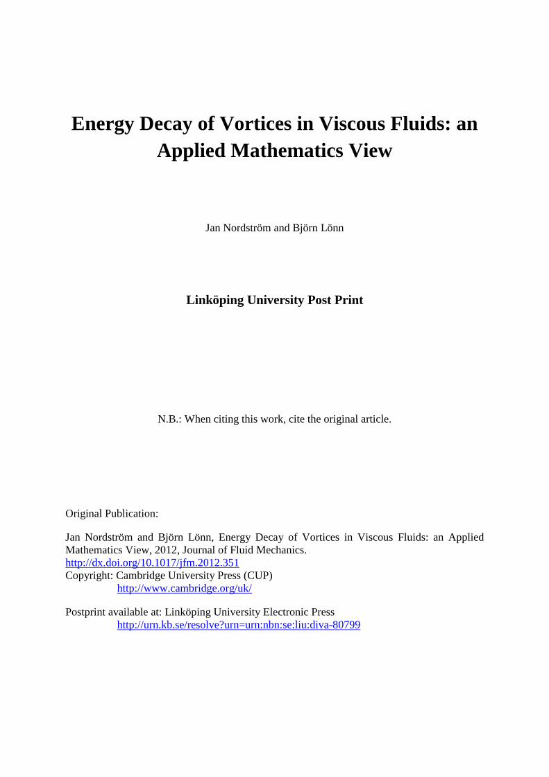
Figure 1: The initial field for the vortex. The velocities decrease fast outside r=1.

The vortex is a so called wake vortex also used in Winckelmans et al. (2006). Theinitial velocity field is shown in Figure 1. It is defined by

uij = − ε · yijx2ij + y2

ij + r2c

vij =ε · xij

x2ij + y2

ij + r2c

(3.1)

where xij , yij are the distances from the center of the vortex in each direction, rc is thedistance from the center to the strongest velocity of the vortex and ε = 2 ∗ rc ∗M . Forcompleteness we also give the velocity components in cylindrical coordinates as

Uθ =εr

r2 + r2c

Ur = 0 (3.2)

where r =√x2 + y2 is the radius and Uθ, Ur are the tangential and radial velocities

respectively.The initial velocity field of the white noise is shown in Figure 2. It is defined by

uij =ε · randomx2ij + y2

ij + r2c

vij =ε · randomx2ij + y2

ij + r2c

rand ∈ [−1, 1] (3.3)

where ε is the same as in (3.1). The velocities are randomized using random numbersfrom the Fortran 90 random subroutine and damped to zero using the same function asthe vortex condition. The velocities in cylindrical coordinates are

Uθ(r, θ) =ε random

r2 + r2c

, Ur(r, θ) =ε random

r2 + r2c

(3.4)

with the same definitions as in (3.2).In all the calculations in this paper, the Mach number is small, and the initial condition

should (almost) satisfy the zero divergence relation in incompressible flow. However, the


x

y

-10 -5 0 5 10-10

-8

-6

-4

-2

0

2

4

6

8

10

Figure 2: The initial field for the white noise. The velocities decrease fast outside r=1.

x

y

-10 -5 0 5 10-10

-5

0

5

10

Figure 3: The initial field for the divergence free case. The velocities decrease fast outsider=1.


x

y

-10 -5 0 5 10-10

-8

-6

-4

-2

0

2

4

6

8

10

(a) t=50

x

y

-10 -5 0 5 10-10

-8

-6

-4

-2

0

2

4

6

8

10

(b) t=1000

x

y

-10 -5 0 5 10-10

-8

-6

-4

-2

0

2

4

6

8

10

(c) t=4000

Figure 4: Time evolution of the vortex for Re=1000. The radius is displayed by the lowdensity core indicated with dark blue. As time passes, the velocities slowly weaken.

white noise do not have zero divergence. In order to check if that has any impact on theresults, we included a special zero divergence initial condition shown in Figure 3 of thefollowing form

uij = εxij + yij

exp [(xij + yij)2 + r2c ]

vij = −ε xij + yijexp [(xij + yij)2 + r2

c ]. (3.5)

Here ε is the same as in (3.1). When r > 1 we replace the denominator exp [(xij + yij)2 +r2c ] with exp [x2

ij + y2ij + r2

c ] for a fast decay of the solution. The formulation (3.5) incylindrical coordinates is

Uθ(r, θ) = εh(r, θ)cos(θ + 3π/4), Ur(r, θ) = εh(r, θ)sin(θ + 3π/4) (3.6)

where h(r, θ) = r(cos(θ) + sin(θ))/ exp(r2(cos(θ) + sin(θ))2 + r2c ).

3.3. Time evolution

The time evolution of the vortex can be seen in Figure 4. The kinetic energy of the vortexspread evenly to the area surrounding it. At t=4000 the vortex seems only slightly weaker.In an isolated vortex one has an inner vortex core (r < rc) which is rotating as a solidbody. In the outer part (r > rc), both the strain rate (with non-zero eigenvalues) and thevorticity is present, see the first remark in section 2.2. Thus, the vortex will be dampedfrom outside leaving the vortex core undamped but with a shrinking core radius. This isexactly what is seen in Figure 4, and also consistent with the finding of Wallin & Girimaji(2000) for turbulent decay of wing tip vortices.

The white noise computation is displayed in Figure 5. It decays quickly and has almostvanished at t=1000. A closer look at what remain of the white noise at t=400 andt=1000 reveal several vorticity like flow structures. The time development of the specialdivergence free case is displayed in Figure 6. The flow develops into two counter clockwiserotating vortices. These vortices remain for a long time and decay slowly.

Remark: The result of these three calculations is consistent with the theory in Section2. The fact that even if one starts the calculation with a non-vortex structure (as inFigures 5 and 6), one ends up with only vortex like structures is particularly striking.This could be a scenario in which energy is transferred from non-vorticity modes tovorticity modes as mentioned earlier.


x

y

-10 -5 0 5 10-10

-8

-6

-4

-2

0

2

4

6

8

10

(a) t=8

x

y

-10 -5 0 5 10-10

-8

-6

-4

-2

0

2

4

6

8

10

(b) t=400

x

y

-10 -5 0 5 10-10

-8

-6

-4

-2

0

2

4

6

8

10

(c) t=1000

x

y

-4 -2 0 2 4

-4

-2

0

2

4

(d) t=400 zoomed

x

y

-4 -2 0 2 4

-4

-2

0

2

4

(e) t=1000 zoomed

Figure 5: Time evolution of the white noise for Re=1000. The white noise decays quickly.At t=400 and t=1000 only vorticity like flow structures remain.

3.4. Energy decay

The kinetic energy of the global system E = ρu2+v2+w2

2 as a function of time, normalizedby the initial kinetic energy, is shown in Figure 7. The energy decay of white noise isclearly faster than the energy decay of the wake vortex and the divergence free flow case.The fast decay is predicted by the theory since white noise has large gradients initiallycompared to the other initial conditions. Note that once the white noise has developedinto a flow consisting mainly of vorticity, see Figure 5, the decay stops.

The energy of the vortex decrease slowly with time which agrees with the resultsobtained in Winckelmans et al. (2006). Despite the fact that the wake vortex flow withRe=100 looks weaker at t=4000 more than 90% of the kinetic energy in the global systemremain.

The energy decay of the divergence free case is faster than the vortex energy decay butslower than the white noise energy decay. The decay is semi-fast initially when the velocity


x

y

-10 -5 0 5 10-10

-5

0

5

10

(a) t=7

x

y

-10 -5 0 5 10-10

-5

0

5

10

(b) t=1000

x

y

-10 -5 0 5 10-10

-5

0

5

10

(c) t=4000

Figure 6: Time evolution of the divergence free case for Re=1000. A wave leaves thedomain at t=10. The remaining counter clockwise rotating vortices decay slowly.

0 1000 2000 3000 4000 50000

0.1

0.2

0.3

0.4

0.5

0.6

0.7

0.8

0.9

1

Dimensionless Time (t)

Norm

alize

d Kine

tic E

nerg

y (E/

E 0)

Wake vortex Re=1000Wake vortex Re=100Wake vortex Re=10Div. Free Re=1000Div. Free Re=100Div. Free Re=10White noise Re=1000White noise Re=100White noise Re=10

Figure 7: Normalized kinetic energy decay for the 2D vortex, divergence free and whitenoise cases as a function of time. The vortex has the least energy decay.

gradients are strong and decreases as the flow becomes dominated by the two counterrotating vortices. Once the vortices have formed, the decay slow down significantly.

For all three cases, computing with a lower/higher Reynolds number consistently re-sulted in more/less energy decay for all three cases.

Remark: The result of the calculations, i.e that vortex like structures decay slowlyand other flow structures relatively fast is consistent with the theory in Section 2. Theresults are also consistent with the asymptotic decay rates obtained in Hoff & Zumbrum(1995) for the Cauchy problem, if one takes into account the fact that we are computingon a finite domain. (On a finite domain, the acoustic part will radiate to infinity anddecay rapidly). The results of Hoff & Zumbrum (1995) also indicate that the transfer ofenergy between the vorticity modes and other modes is small, which again is consistentwith our computational results.


0 100 200 300 400 5000

0.1

0.2

0.3

0.4

0.5

0.6

0.7

0.8

0.9

1

Dimensionless Time (t)

Norm

alize

d Kine

tic E

nerg

y (E/

E 0)

Wake vortex Re=10Div. Free Re=10White noise Re=10

Figure 8: Normalized kinetic energy decay for the 3D vortex, divergence free and whitenoise cases as a function of time. The vortex has the least energy decay also in 3D.

3.5. Validation of the resultsTo confirm the results obtained in two dimensions, also three dimensional calculationswere made. The initial velocities are defined as:

V ortex : uijk =−ε · yijkf(x, y, z)

, vijk =ε · xijkf(x, y, z)

, wijk = 0 (3.7)

White noise : uijk =ε · randomf(x, y, z)

, vijk =ε · randomf(x, y, z)

, wijk = 0 (3.8)

Divergence free : uij = εxij + yijg(x, y, z)

, vij = −ε xij + yijg(x, y, z)

, wijk = 0 (3.9)

where f(x, y, z) = x2ijk + y2

ijk + z2ijk + r2

c and g(x, y, z) = exp [(xij + yij + zij)2 + r2c ]. The

same parameter values as in two dimensions were used. Note that the flow is truly threedimensional due to the z-dependence in f(x, y, z) and g(x, y, z) even though the velocityin the z-direction is initially zero. Note also that (3.9) is, strictly speaking, no longerdivergence free due to the z dependence.

The focus of the computations in three dimensions is to verify the relevance of thecomputations in two dimensions. Far field boundary conditions are used on all outerboundaries, except in the z-direction where periodic boundary conditions are used.

The energy of the global system as a function of time is shown in Figure 8. In allthree computations the energy decay is similar to and hence validate the energy decayobtained from the two dimensional computations.

4. DiscussionThe main result of the mathematical analysis, relation (2.13), describes how the dis-

turbance energy (the deviation from the constant background field) decay (or do notdecay). The right hand side of (2.13) is diagonalised such that each eigenvalue multipliesa quadratic form. Each quadratic form, shown in (2.14), consists of linear combinations


of the gradients of the flow variables. The eigenvalues and quadratic forms can be or-ganized in two groups. Group one has non-zero positive eigenvalues and group two haszero eigenvalues and correspond exactly to the vorticity modes. For easy of explanationwe denote the modes in group one, the ’decay’ modes.

We start by considering the energy decay only. Firstly, assume that all the quadraticforms/modes are non-zero. Due to the non-zero eigenvalues related to the ’decay’ modes,we have energy decay. Secondly, assume that the ’decay’ modes are zero, while the vor-ticity modes are non-zero. Then, since the eigenvalues related to the vorticity modes arezero, the energy will stay constant even though the corresponding quadratic forms/modesare non-zero. Note that if all the eigenvalues were non-zero, no possibility for a constantenergy would exist.

Now we include energy transfer in the discussion. Consider the second case above whichat a particular time do not yield energy decay, i.e. all the energy reside in the vorticitymodes. If the energy from the the vorticity modes is transferred to the ’decay’ modes, wehave energy decay in the next instant. If the transfer is large, we will have a large decay,if the transfer is small we will have a small decay. The reversed scenario is also possible,i.e. that energy may transfer from ’decay’ modes to vorticity modes which will decreasethe energy decay from a high level to a low level.

The results discussed above have implications for the practical treatment (both theremoval and the preservation) of energy content in flow structures. For a general flowstructure from which one wants to remove energy, one could aim for transferring energyfrom the vorticity modes into the ’decay’ modes, and use the natural decay mechanismdiscovered in this paper as guidance.

5. ConclusionsWe have analysed the energy decay of small scale disturbances in laminar flow by using

the energy-method. An equation for the energy decay rate in terms of gradients and adissipation matrix was derived. Zero eigenvalues of the dissipation matrix multiplied thevorticity components.

The zero eigenvalues multiplying the vorticity components suggest that flows withmost of the energy in the vorticity components decay slowly. It also mean that smallscale disturbances will have most of their energy in vorticity form after a long time.

Numerical simulations verified that the energy decay is slow for vortices compared tothe white noise and divergence free flow cases. The simulations also verified that theenergy transfer from the vorticity components to other modes is slow, leading to a slowoverall decay.

The existence of zero eigenvalues multiplying the vorticity component of the flow isprobably one of the main reasons for the slow decay of energy in vortex like structuresin fluid mechanics.

The energy transfer between vorticity modes and non-vorticity modes was investigatednumerically. This part could possibly be improved by an even more advanced analysisand we hope that the finding in this paper will inspire others to do that.

REFERENCES

Abarbanel, S. & Gottlieb, D. 1981 Optimal time splitting for two- and three-dimensionalNavier-Stokes equations with mixed derivatives. Journal of Computational Physics 41 (1),1–33.

Anderson, J. D. 1991 Fundamentals of Aerodynamics, 2nd edition. McGraw-Hill, Inc.


Balmforth, NJ, Smith, SGL & Young, WR 2001 Disturbing vortices. Journal of FluidMechanics 426, 95–133.

Beggs, P. J., Selkirk, P. M. & Kingdom, D. L. 2004 Identification of von karman vorticesin the surface winds of heard island. Boundary-Layer Meteorology 113 (2), 287–297.

Breitsamter, C. 2011 Wake vortex characteristics of transport aircraft. Progress in AerospaceSciences 47 (2), 89–134.

Carpenter, M. H., Nordstrom, J. & Gottlieb, D. 1999 A stable and conservative interfacetreatment of arbitrary spatial accuracy. Journal of Computational Physics 148 (2), 341–365.

Chen, K. K., Colonius, T. & Taira, K. 2010 The leading-edge vortex and quasisteady vortexshedding on an accelerating plate. Physics of Fluids 22 (3), 1–11.

Davoudzadeh, F., McDonald, H. & Thompson, B. E. 1995 Accuracy evaluation of unsteadycfd numerical schemes by vortex preservation. Computers and Fluids 24 (8), 883–895.

Erlebacher, G., Hussaini, M. Y. & Shu, C. W. 1997 Interaction of a shock with a longitu-dinal vortex. Journal of Fluid Mechanics 337, 129–153.

Gerz, T & Holzapfel, F 1999 Wing-tip vortices, turbulence, and the distribution of emissions.AIAA Journal 37 (10), 1270–1276.

Gerz, T, Holzapfel, F & Darracq, D 2002 Commercial aircraft wake vortices. Progress inAerospace Sciences 38 (3), 181–208.

Greene, GC 1986 An Approximate Model for Vortex Decay in the Atmosphere. Journal ofAircraft 23 (7), 566–573.

Gustafsson, B., Kreiss, H. O. & Oliger, J. 1995 Time Dependent Problems and DifferenceMethods. Academic Press.

Gustafsson, B & Sundstrom, A 1978 Incompletely Parabolic Problems in Fluid-Dynamics.SIAM Journal on Applied Mathematics 35 (2), 343–357.

Gustavsson, LH 1991 Energy Growth of 3-Dimensional Disturbances in Plane Poiseuille Flow.Journal of Fluid Mechanics 224, 241–260.

Hagstrom, T. & Lorenz, J. 1995 All-time existence of smooth solutions to PDEs of mixedtype and the invariant subspace of uniform states. Advances in Applied Mathematics 16,219–257.

Hagstrom, T. & Lorenz, J. 2002 On the stability of approximate solutions of hyperbolic-parabolic systems and the all-time existence of smooth, slightly compressible flows. IndianaUniviversity Mathematics Journal 51, 1339–1387.

Hoff, D. & Zumbrum, K. 1995 Multidimensional diffusion waves for the Navier-Stokes equa-tions of compressible flow. Indiana Univiversity Mathematics Journal 44 (2), 603–676.

Holland, W. R. 1978 The role of mesoscale eddies in the general circulation of the ocean -numerical experiments using a wind-driven quasi-geostrophic model. Journal of PhysicalOceanography 8, 363–392.

Holzapfel, F, Hofbauer, T, Darracq, D, Moet, H, Garnier, F & Gago, CF 2003 Anal-ysis of wake vortex decay mechanisms in the atmosphere. Aerospace Science and Technology7 (4), 263–275.

Kantha, L. 2010 Decay of Aircraft Wake Vortices Under Daytime Free Convective Conditions.Journal of Aircraft 47 (6), 2159–2164.

Kim, J-H. & Kim, C. 2011 Computational Investigation of Three-Dimensional Unsteady Flow-field Characteristics Around Insects’ Flapping Flight. AIAA Journal 49 (5), 953–968.

Koszalka, I., LaCasce, J. H., Andersson, M., Orvik, K. A. & Mauritzen, C. 2011Surface circulation in the Nordic Seas from clustered drifters. Deep-Sea Research Part I-Oceanographic Research Papers 58 (4), 468–485.

Kreiss, H. O. & Lorenz, J. 1989 Initial Boundary Value Problems and the Navier-StokesEquations. John Wiley & Sons.

Kundu, P. & Cohen, I. 2001 Fluid mechanics, 2nd edition. Elsevier Academic Press.

Liu, Y., Liu, N. & Lu, X. 2009 Numerical Study of Two-Winged Insect Hovering Flight.Advances in Applied Mathematics and Mechanics 1 (4), 481–509.

Magnusson, M. & Smedman, A. 1999 Air flow behind wind turbines. Journal of Wind Engi-neering and Industrial Aerodynamics 80 (1-2), 169–189.

Matthaeus, WH, Stribling, WT, Martinez, D, Oughton, S & Montgomery, D 1991


Decaying, 2-Dimensional, Navier-Stokes Turbulence at Very Long Times. Physica D 51 (1-3), 531–538.

Mattsson, K, Svard, M & Nordstrom, J 2004 Stable and accurate artificial dissipation.Journal of Scientific Computing 21 (1), 57–79.

McCormack, P. D. & Crane, L. 1973 Physical Fluid Dynamics. Academic press.Nordstrom, J 1995 The Use of Characteristic Boundary-Conditions for the Navier-Stokes

Equations. Computers & Fluids 24 (5), 609–623.Nordstrom, J. & Carpenter, M.H. 1999 Boundary and interface conditions for high-order

finite-difference methods applied to the Euler and Navier-Stokes equations. Journal ofComputational Physics 148, 621–645.

Nordstrom, J. & Carpenter, M. H. 2001 High-order finite difference methods, multidi-mensional linear problems, and curvilinear coordinates. Journal of Computational Physics173 (1), 149–174.

Nordstrom, J., Gong, J., van der Weide, E. & Svard, M. 2009 A stable and conservativehigh order multi-block method for the compressible Navier-Stokes equations. Journal ofComputational Physics 228 (24), 9020–9035.

Nordstrom, J. & Svard, M. 2005 Well-posed boundary conditions for the navier-stokes equa-tions. SIAM Journal on Numerical Analysis 43, 1231–1255.

Ponta, F. L. 2010 Vortex decay in the Karman eddy street. Physics of Fluids 22 (9).Proctor, F. H. 1998 The NASA-Langley wake vortex modelling effort in support of an op-

erational aircraft spacing system, AIAA paper 98-0589. In 36th AIAA Aerospace SciencesMeeting and Exhibit .

Pullin, DI & Saffman, PG 1998 Vortex dynamics in turbulence. Annual Review of FluidMechanics 30, 31–51.

Rossow, VJ 1999 Lift-generated vortex wakes of subsonic transport aircraft. Progress inAerospace Sciences 35 (6), 507–660.

Sarpkaya, T 1998 Decay of wake vortices of large aircraft. AIAA Journal 36 (9), 1671–1679.Spalart, PR 1998 Airplane trailing vortices. Annual Review of Fluid Mechanics 30, 107–138.Svard, M., Carpenter, M. H. & Nordstrom, J. 2007 A stable high-order finite difference

scheme for the compressible Navier-Stokes equations, far-field boundary conditions. Journalof Computational Physics 225 (1), 1020–1038.

Svard, M. & Nordstrom, J. 2008 A stable high-order finite difference scheme for the compress-ible Navier-Stokes equations. No-slip wall boundary conditions. Journal of ComputationalPhysics 227 (10), 4805–4824.

Wallin, S. & Girimaji, SS. 2000 Evolution of an isolated turbulent trailing vortex. AIAAJournal 38 (4), 657–665.

White, F. M. 1974 Viscous Fluid Flow . McGraw-Hill, Inc.Winckelmans, G., Cocle, R., Dufresne, L., Capart, R., Bricteux, L., Daeninck, G.,

Lonfils, T., Duponcheel, M., Desenfas, O. & Georges, L. 2006 Direct numericalsimulation and large-eddy simulation of wake vortices: Going from laboratory conditionsto flight conditions. In In European Conference on Computational Fluid Dynamics, EC-COMAS CFD .

Winter, B. & Bourqui, M. S. 2011 The impact of surface temperature variability on theclimate change response in the Northern Hemisphere polar vortex. Geophysical ResearchLetters 38.

Wu, T. Y. 2011 Fish Swimming and Bird/Insect Flight. In Annual Review of Fluid Mechanics,Annual Review of Fluid Mechanics, vol. 43, pp. 25–58.

Yen, S-C. 2011 Aerodynamic Performance and Shedding Characteristics on a Swept-back Wing.Journal of Marine Science and Technology-TAIWAN 19 (2), 162–167.

Zhang, Y., Pedlosky, J. & Flierl, G. R. 2011 Shelf Circulation and Cross-Shelf Transportout of a Bay Driven by Eddies from an Open-Ocean Current. Part I: Interaction betweena Barotropic Vortex and a Steplike Topography. Journal of Physical Oceanography 41 (5),889–910.

Zhou, J, Adrian, RJ, Balachandar, S & Kendall, TM 1999 Mechanisms for generatingcoherent packets of hairpin vortices in channel flow. Journal of Fluid Mechanics 387, 353–396.

Energy Decay of Vortices in Viscous Fluids: an Applied ...

Documents

Transcript of Energy Decay of Vortices in Viscous Fluids: an Applied ...