Energy Consumption Of Visual Sensor Networks:

Impact Of Spatio-Temporal Coverage Based On

Single-Hop Topologies

Alessandro Redondi1, Dujdow Buranapanichkit2, Matteo Cesana1, MarcoTagliasacchi1 and Yiannis Andreopoulos3

1Electronic, Information and Bioengineering Department, Politecnico di Milano, Italy{redondi,cesana,tagliasa}@elet.polimi.it

2Department of Electrical Engineering, Prince of Songkla University, Thailanddujdow.b@psu.ac.th

3Electronic and Electrical Engineering Department, University College London, UKi.andreopoulos@ucl.ac.uk

Abstract. Wireless visual sensor networks (VSNs) are expected to playa major role in future IEEE 802.15.4 personal area networks (PAN) underrecently-established collision-free medium access control (MAC) proto-cols. In such environments, the trade-o� between the number of camerasensors to deploy (spatial coverage) and the frame rate to use for eachcamera sensor (temporal coverage) plays a major role in the VSN en-ergy consumption. In this paper, we address this aspect for single-hopVSNs, i.e. networks comprising independent and identical wireless vi-sual sensor nodes connected to a collection node via a star topology. Wederive analytic results for the energy-optimal spatio-temporal coverageparameters of such VSNs under a-priori known bounds for the mini-mum frame rate per sensor and the minimum and maximum possiblenumber of nodes to deploy. Our results are parametric to the probabilitydensity function characterizing the data-production rate per node andthe energy consumption parameters of the system of interest. Experi-mental results using TelosB motes under: a collision-free transmissionprotocol, the IEEE 802.15.4 PAN physical layer (CC2420 transceiver)and Monte-Carlo�generated data sets, reveal that our analytic resultsare within 7% of the energy consumption measurements for a wide rangeof settings. In addition, results obtained via a multimedia subsystem per-forming visual feature extraction in video frames show that the optimalspatio-temporal settings derived by the proposed framework allow forup to 48% of reduction of energy consumption in comparison to ad-hocsettings. As such, our analytic modeling is useful for early-stage studiesof possible VSN deployments under collision-free MAC protocols priorto costly and time-consuming experiments in the �eld.

1 Introduction

The integration of low-power wireless networking technologies such as IEEE802.15.4-enabled transceivers [1] with inexpensive camera hardware [2] has en-abled the development of the so-called visual sensor networks (VSNs). VSNs

can be thought of as networks of wireless devices capable of sensing multime-dia content [3], such as still images and video, audio, depth maps, etc. Via therecent provisioning of an all-IPv6 network layer under 6LoWPAN and the emer-gence of collision-free low-power medium access control (MAC) protocols, suchas the time slotted channel hopping (TSCH) of IEEE 802.15.4e-2012 [4], VSNsare expected to play a major role in the evolution of the Internet-of-Things (IoT)paradigm [5].

1.1 Review of Visual Sensor Networks

An increasing number of VSN solutions were proposed recently with a focuson new transmission protocols allowing for high-bandwidth collision-free com-munications [6,4] and in-network visual processing techniques [7]. Most of theproposed VSN solutions can be abstracted as two tightly-coupled subsystems: amultimedia processor board and a low-power radio subsystem [2], interconnectedvia a push model. A cluster of such identical nodes can be organized into a VSNcomprising a star topology that can operate in collision-free steady-state modeas illustrated in the example of Figure 1, with the consumption rate of each nodebeing s bits for each interval of T seconds that the VSN remains active, or s

Tbits-per-second (bps). Within each node, the multimedia subsystem is respon-sible for acquiring images, processing them and pushing the processed data tothe radio subsystem. For example, in the most typical application scenario forVSNs, the multimedia subsystem would acquire each image, compress it into aJPEG bitstream (e.g., using an MJPEG codec) and push the JPEG bitstreamto the radio subsystem [2]. The latter transmits the processed data stream tothe low-power border router (LPBR) [5], and eventually to a remote destination,which, under the IoT paradigm, could be any IPv6 Internet address.

Multimedia processing subsystem: The frame rate under which each VSNcamera is operating, i.e. each node's temporal coverage, is controlling the fre-quency of the push operations. At the same time, the multimedia processing taskitself (e.g., JPEG compression) controls the volume of bits pushed to the radiosubsystem within each frame's duration.

Communications subsystem: The number of sensors in the (single-hop) startopology, i.e. the VSN's spatial coverage (Figure 1), controls the bandwidthavailable to each sensor (i.e. its average transmission rate) under a collision-freeMAC protocol [6,8,4]. Thus, there is a fundamental tradeo� between the spatialand temporal coverage in a network: high frame rate leads to high bandwidthrequirement per transmitter, which in turn decreases the number of sensors thatcan be accommodated with the same LPBR. Conversely, dense spatial coveragevia the use of a large number of visual sensors decreases the available bandwidthper sensor and this in turn reduces the achievable frame rate per sensor in orderto maintain tight coupling.

LPBR

s/4s/4

s/4 s/4

Radio Subsystem

Multimedia Subsystem

Memory

Camera

Raw image data

JPEG image / salient points

Data buffering

Data transmissionto higher tier / LPBR

Fig. 1. Single-hop star topology in a visual sensor network, where every visual sensor(video camera) has its own spatial coverage, with s indicating the bits consumed byeach node within each active interval of T seconds. Each camera node comprises twosubsystems, which are illustrated in the �gure expansion. If required, each node canbu�er parts of its data stream for later transmission.

Overall system perspective � energy consumption: Like traditional wire-less sensor networks, VSN nodes are battery operated. Hence, energy consump-tion plays a crucial role in the design of a VSN, especially for those applicationswhere a VSN is required to operate for days or even weeks without externalpower supply. In the last few years, several works have addressed the problemof lifetime maximization in VSNs: depending on the research area, solutions areavailable for energy-aware protocols and cross-layer optimization [4], applicationtradeo�s [5] and deployment strategies [2]. While existing work addresses trans-mission, scheduling and protocol design aiming for energy e�ciency, it does notconsider the impact of the spatio-temporal coverage in the energy consumptionof VSNs. This is precisely the focus of this paper.

1.2 Contribution

In this paper, we derive analytic results concerning energy-aware VSN deploy-ments under the push model of Figure 1. Speci�cally, we are interested in thelink of the aforementioned spatio-temporal tradeo� with the incurred energy con-sumption under well known probability density functions modeling the pusheddata volume of image and video applications, such as intra/inter-frame videocoding and visual features extraction and transmission. We focus on the widelyused case of single-hop VSNs comprising identical sensors connected to the LPBRvia a star topology and we derive an analytic model that captures the expectedenergy consumption in function of: (i) the number of visual sensors deployed,(ii) the frame rate used by each camera sensor and (iii) the statistical charac-terization of the bitstream data volume produced by each sensor after on-boardimage analysis or compression. The extrema of the derived energy consumption

function are then analytically derived in order to provide closed-form expressionsfor the minimum energy consumption of each case under consideration. The de-rived analytic results are experimentally validated with a VSN performing visualfeature extraction and transmission to the LPBR.

2 Utilized System Model and Its Expected Energy

Consumption

In the �rst four subsections we introduce the components of the utilized systemmodel and the corresponding nomenclature. The key notations are summarizedin Table 1, along with the practical settings used in the experiments of the paper.

2.1 Communication and System Infrastructure

Consider a wireless visual sensor network comprising a star topology. The net-work consists of n independent and identical camera nodes that process visualdata and transmit multimedia streams to the LPBR. The MAC layer of the net-work is operating under a collision-free time-division (or time-frequency division)multiple access protocol [6,8,4], so that simultaneous transmissions (self-in�ictedcollisions) are avoided. Let s

T bps be the average consumption rate of the LPBRover the VSN active interval of T seconds.

Within each node, the multimedia and radio subsystems work in parallel:while the multimedia system acquires and processes data corresponding to thecurrent video frame, the radio subsystem transmits the multimedia stream stem-ming from the processing of the previous video frame(s). Examples of VSN ap-plications that �t the communications model illustrated in Figure 1 are: multi-camera JPEG compression and transmission of video bitstreams [7], multi-sensorvisual features extraction [9] and transmission, multi-camera compression andtransmission for object recognition, etc.

2.2 Active Time Interval and Delay Tolerance

Given that applications based on visual sensor networks are subject to severebandwidth requirements, it may not be possible to transmit the entirety of eachmultimedia stream within the transmission opportunities corresponding to theduration of one video frame. In such a case, bu�ering to on-board memory isrequired. This means that the application must tolerate certain delay until allmultimedia streams are received by the LPBR. This delay is controlled by thechosen value of T and can be tuned to �t the constraints imposed by eachdeployment scenario.

After T seconds, each sensor stops gathering new data, completes the trans-mission of any data that may exist in its bu�er and goes into suspension modeuntil the occurrence of the next active time interval. For example, setting T = 5s indicates that the sensors are actively gathering and processing visual data for�ve seconds, complete any remaining data transmissions after that, and then

suspend their activity until being reactivated. The VSN activation can eitherbe event-driven (e.g., when activity or motion is detected) or periodic, with acertain duty cycle [2,4].

2.3 Spatio-Temporal Coverage and Statistical Characterization of

Data Transmission Volume per VSN Node

We consider that the VSN is established under the following two applicationconstraints:

� spatial coverage bounds; the number of deployed nodes, n, is upper- andlower-bounded, i.e., Nmin ≤ n ≤ Nmax

� temporal coverage lower bound ; the total frame acquisitions, k, within a pre-de�ned time interval, T , is lower-bounded, i.e., k ≥ Kmin

The bounds of the spatio-temporal coverage stem from application speci�cs,such as: the cost of installing and maintaining visual sensors, the minimumand maximum spatial coverage required for the area to be monitored, and theminimum frame rate that allows for visual data gathering and analysis withsu�cient temporal resolution for the application.

Since the multimedia subsystem of each visual sensor produces varying amountsof data depending on the monitored events and the speci�cs of the visual anal-ysis and processing under consideration, the data stream volume produced byeach camera in such multimedia applications is a non-deterministic quantity. Wethus model the data volume produced when each camera processes k frames viaa random variable (RV) Xk, with marginal probability density function (PDF)P (χk), Xk v P (χk) [10].

2.4 Energy Consumption Penalties

Following the push model illustrated in Figure 1, each node performs the follow-ing operations during the active time interval T :

1. Acquisition: A low-power camera sensor acquires k frames, each incurring aJoule (J) of energy expenditure. Hence, the energy consumed during T s iska J.

2. Processing and transmission: Each captured video frame is processed with aCPU-intensive algorithm, realized by the multimedia subsystem. Each frameprocessing produces, on average, r bits (b) for transmission. These bits arepushed to the radio subsystem, which in turn transmits them to the basestation. Let g J be the average energy required for processing and producingone bit of information and j the average energy required to transmit it tothe LPBR. The average energy consumed for processing and transmissionwithin the active interval is hence (g + j)

´∞0χkP (χk)dχ = (g + j)E [Xk] J,

with E [Xk] bits comprising the statistical expectation of the data volumecorresponding to k frames.

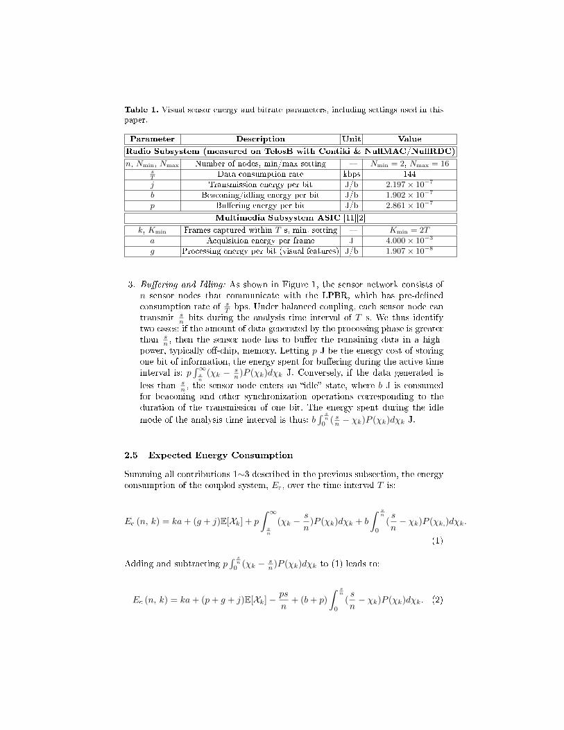
Table 1. Visual sensor energy and bitrate parameters, including settings used in thispaper.

Parameter Description Unit Value

Radio Subsystem (measured on TelosB with Contiki & NullMAC/NullRDC)

n, Nmin, Nmax Number of nodes, min/max setting � Nmin = 2, Nmax = 16sT

Data consumption rate kbps 144

j Transmission energy per bit J/b 2.197× 10−7

b Beaconing/idling energy per bit J/b 1.902× 10−7

p Bu�ering energy per bit J/b 2.861× 10−7

Multimedia Subsystem ASIC [11][2]

k, Kmin Frames captured within T s, min. setting � Kmin = 2T

a Acquisition energy per frame J 4.000× 10−3

g Processing energy per bit (visual features) J/b 1.907× 10−8

3. Bu�ering and Idling: As shown in Figure 1, the sensor network consists ofn sensor nodes that communicate with the LPBR, which has pre-de�nedconsumption rate of s

T bps. Under balanced coupling, each sensor node cantransmit s

n bits during the analysis time interval of T s. We thus identifytwo cases: if the amount of data generated by the processing phase is greaterthan s

n , then the sensor node has to bu�er the remaining data in a high-power, typically o�-chip, memory. Letting p J be the energy cost of storingone bit of information, the energy spent for bu�ering during the active timeinterval is: p

´∞sn

(χk − sn )P (χk)dχk J. Conversely, if the data generated is

less than sn , the sensor node enters an �idle� state, where b J is consumed

for beaconing and other synchronization operations corresponding to theduration of the transmission of one bit. The energy spent during the idle

mode of the analysis time interval is thus: b´ sn

0( sn − χk)P (χk)dχk J.

2.5 Expected Energy Consumption

Summing all contributions 1∼3 described in the previous subsection, the energyconsumption of the coupled system, Ec, over the time interval T is:

Ec (n, k) = ka+ (g + j)E[Xk] + p

ˆ ∞sn

(χk −s

n)P (χk)dχk + b

ˆ sn

0

(s

n− χk)P (χk,)dχk.

(1)

Adding and subtracting p´ sn

0(χk − s

n )P (χk)dχk to (1) leads to:

Ec (n, k) = ka+ (p+ g + j)E[Xk]− ps

n+ (b+ p)

ˆ sn

0

(s

n− χk)P (χk)dχk. (2)

The last equation forms the basis for the analytic exploration of the minimum en-ergy consumption under the knowledge of the marginal PDF [10] characterizingthe data production and transmission process.

3 Analytic Derivation of Minimum Energy Consumption

Our objective is to derive the spatio-temporal parameters minimizing Ec (n, k)in (2) subject to the spatio-temporal constraints de�ned in Section 2, that is:

{n?, k?} = argmin∀n,k

Ec (n, k) , (3)

with

Nmin ≤ n ≤ Nmax and k ≥ Kmin (4)

and {n?, k?} the values deriving the minimum energy consumption.In the following, we consider two di�erent marginal distributions for P (χk)

and derive the choice for n and k that minimizes the energy consumption, whileensuring the conditions imposed by the application constraints are met. Whileour analysis is assuming that n and k are continuous variables, once the {n?, k?}values are derived, they can be discretized to the sets {bn?c , bk?c}, {dn?e , dk?e}{dn?e , bk?c} {bn?c , dk?e} [if all four satisfy the constraints of (4)] in order tocheck which discrete pair of values derives the minimum energy consumption in(2). This is because: (i) the energy functions under consideration are continuousand di�erentiable; and (ii) we shall show that, for the data size PDFs underconsideration, a unique minimum is found for (2) that is parametric to thesetting of the temporal constraint (Kmin). As such, the analysis on the continuousvariable space can be directly mapped onto the discrete variable set under theaforementioned discretization.

3.1 Illustrative Case: Uniform Distribution

When one has limited or no knowledge about the cumulative data transmittedby each VSN node during T , one can assume that P (χk) is uniform over theinterval [0, 2kr]. That is,

P (χk) =

{1

2kr 0 ≤ χk ≤ 2kr

0 otherwise(5)

with EU[Xk] = kr corresponding to the mean value of the data transmitted bya node that produces k frames of r bits each on average. Using (5) in (2) leadsto:

Ec,U(n, k) = k [a+ r(p+ j + g)]− ps

n+s2(b+ p)

4n2kr. (6)

To obtain the solution to (3) under the energy consumption given by (6), onecan search for critical points of Ec,U. Imposing that the derivatives of Ec,U withrespect to n and k are both equal to zero leads to:{

∂Ec,U

∂n = psn2 − s2(b+p)

2n3kr = 0∂Ec,U

∂k = a+ r(p+ j + g)− s2(b+p)4n2k2r = 0

(7)

It can be shown that the solution of (7) requires a < 0 (the detailed derivationis omitted due to space limitations). However, this is not physically feasible sincea is the energy cost to acquire one frame. Hence, under the physical constraintsof the problem, there is no single (global) solution {n?, k?} ∈ R× R to (3) in itsunconstrained form, i.e. when one ignores the constraints of (4). However, wemay look at one or the other direction individually (i.e., along n or k) in orderto �nd a local or global minimum for that particular direction and then choosefor the other direction the value that minimizes (3) under the spatio-temporalconstraints of (4). Subsequently, we can identify if the derived minima are uniqueunder the imposed constraints and whether the entire region of support of theenergy function has been covered by the derived solutions. These are investigatedin the following.

n-direction We examine the function Ec,U along the plane k = k̄, k̄ ≥ Kmin,and analyze Ec,U(n, k̄) which is now a function of n only. It is straightforward toshow by �rst-derivative analysis that the only candidate extremum or in�ectionpoint of Ec,U(n, k̄) is n0,U = βU

k̄, with

βU =s (b+ p)

2pr(8)

de�ned as a �system-speci�c� parameter (which depends on average bits trans-mitted and the energy penalty rates). This candidate extremum or in�ectionpoint is valid under the assumption that: Nmin ≤ n0,U ≤ Nmax, i.e. that the can-didate point falls within the prede�ned spatial constraints of (4). Furthermore,

we �nd thatd2Ec,U(n, k̄)

dn2

∣∣∣n=n0,U

> 0, which demonstrates that n0,U is a local

minimum. Given that local extrema must alternate within the region of sup-port of a continuous and di�erentiable function, the boundary points (n = Nmin

and n = Nmax) cannot be local minima. Thus, n0,U is the global minimum ofEc,U(n, k̄) within Nmin ≤ n ≤ Nmax.

Having derived the global minimum of Ec,U(n, k̄) along an arbitrary planek = k̄, k̄ ≥ Kmin, we can now attempt to �nd the value of k, k ≥ Kmin, thatminimizes the energy function. Evaluating Ec,U(n, k) on n = n0,U we obtain:

Ec,U(n0,U, k) = k

[a+ r

[(p+ j)− p2

b+ p+ g

]]. (9)

Evidently, the value of k minimizing (9) is the minimum allowable, i.e. k = Kmin.

Thus, the solution minimizing (3) in the n-direction is Sn0,U=(

βUKmin

, Kmin

).

This solution holds under the constraint:

Nmin ≤βUKmin

≤ Nmax. (10)

k-direction Similarly, we cut Ec,U(n, k) along the plane n = n̄, Nmin ≤ n̄ ≤Nmax, and minimize Ec,U(n̄, k) which is now function of k only. Following thesteps presented earlier, we can show by �rst and second derivative analysis thatthe global minimum of Ec,U(n̄, k) occurs at k0,U = γU

n̄ with the �system-speci�c�parameter γU de�ned as:

γU =s

2

√b+ p

r [a+ r(p+ j + g)]. (11)

The global minimum of k0,U given above holds under the assumption that k0,U ≥Kmin due the prede�ned temporal constraint of (4). Having derived the globalminimum of Ec,U(n̄, k) along an arbitrary plane n = n̄, Nmin ≤ n̄ ≤ Nmax, wecan now attempt to �nd the value of n, Nmin ≤ n ≤ Nmax, that minimizes theenergy function. Evaluating Ec,U(n, k) on k = k0,U we obtain:

Ec,U(n, k0,U) =1

n

[a+ r(p+ j + g)γU − ps+

s2(b+ p)

4rγU

](12)

Evidently, the value of n minimizing (12) is the maximum allowable, i.e. n =Nmax. Hence, the solution when attempting to minimize (12) in the k-direction

under the constraints of (4) is Sk0,U =(Nmax,

γUNmax

), under the constraint:

Kmin ≤γUNmax

. (13)

Uniqueness of solution and solution when (10) and (13) do not hold:

Starting from (10), with a few straightforward manipulations we reach βUNmax

≤Kmin ≤ βU

Nmin, with βU de�ned in (8). The second constraint for Kmin is provided

by (13). It can be shown that βU > γU (derivation omitted due to page limita-tion), which demonstrates that the constraints of the two established solutionsare non-overlapping. Thus, the solutions Sn0,U

and Sk0,U are unique within theirrespective bounds for Kmin.

To establish the optimal solutions when neither of these two constraints issatis�ed, we have to analyze what happens when γU

Nmax< Kmin < βU

Nmaxor

Kmin > βUNmin

, as neither Sn0,Unor Sk0,U are applicable in such cases. It is

straightforward to show that∂Ec,U

∂n and∂Ec,U

∂k are never zero within these inter-vals. Hence, the solution we are looking for must lie on one of the two boundarypoints: (Nmin,Kmin) or (Nmax,Kmin).

Let's focus on the case of Kmin ∈(

γUNmax

, βUNmax

)and evaluate Ec,U(n, k) on

the boundary plane n = Nmax. Since Ec(Nmax, k) is monotonically increasing for

k > γUNmax

the optimal point is k = Kmin, which leads to the solution Smax min =(Nmax, Kmin). Similarly, let's look at the k direction by evaluating the energyfunction on the k = Kmin plane. Now n0,U = βU

Kminis larger than Nmax and is

thus not admissible. Since Ec,U(n, Kmin) is decreasing for n < n0,U, the optimalpoint is n = Nmax, which also leads to the solution Smax min = (Nmax, Kmin).

Hence we conclude that when Kmin ∈(

γUNmax

, βUNmax

), the optimal solution is

Smax min = (Nmax, Kmin). Finally, when Kmin > βUNmin

, following a similaranalysis we reach that the optimal solution is Smin min = (Nmin, Kmin).

Summarizing, when the data transmitted by each VSN node follows the Uni-form distribution of (5), the set of solutions giving the minimum energy con-sumption in (3) under the spatio-temporal constraints of (4) is:

{n?, k?}U =

(Nmax,

γUNmax

)if Kmin ≤ γU

Nmax

(Nmax, Kmin) if γUNmax

< Kmin <βUNmax(

βUKmin

, Kmin

)if βUNmax

≤ Kmin ≤ βUNmin

(Nmin, Kmin) if Kmin >βUNmin

(14)

with βU and γU de�ned by (8) and (11).

3.2 Pareto Distribution

We present a second example with the Pareto distribution. This distributionhas been used, amongst others, to model the marginal data size distributionof TCP sessions that contain substantial number of small �les and a few verylarge ones [12]. It will also be shown by the experimental results of this paperthat it presents a good �t to multimedia tra�c generated by visual featuresextraction algorithms and hence it warrants detailed study under the proposedVSN framework.

Consider P (χk) as the Pareto distribution with scale v and shape α > 1:

P (χk) =

{α vα

χα+1k

, χk ≥ v

0, otherwise. (15)

Setting v = α−1α kr leads to EP[Xk] = kr, i.e., we match the expected transmis-

sion data volume to that of the Uniform distribution.Under (15), the energy expression of (2) becomes:

Ec,P = k [a+ r(p+ j + g)] +bs

n+ (b+ p)

(vαnα−1

sα−1 (α− 1)− αv

α− 1

). (16)

Following the same analysis as for the Uniform PDF, we conclude that, whenthe data transmitted by each VSN node follows the Pareto distribution of (15),the set of solutions giving the minimum energy consumption in (3) under thespatio-temporal constraints of (4) is:

{n?, k?}P =

(Nmax,

γPNmax

)if Kmin ≤ γP

Nmax

(Nmax, Kmin) if γPNmax

< Kmin <βPNmax(

βPKmin

, Kmin

)if βPNmax

≤ Kmin ≤ βPNmin

(Nmin, Kmin) if Kmin >βPNmin

,

(17)

with

βP =sα

r (α− 1)

(b

b+ p

)1α , (18)

and

γP =sα

r(α− 1)

(r(b− j − g)− a

r (b+ p)

) 1α−1

. (19)

The details of the derivation of (17) follow the same steps as the ones detailedfor the Uniform distribution and are omitted for brevity of description.

3.3 Discussion

The results of this section can be used in practical applications to assess the im-pact of the spatio-temporal constraints and the data production and transmissionprocess (as characterized by its marginal PDF) on the energy consumption ofVSNs, under a variety of energy consumption rates for the radio and multimediasubsystems. For example, under particular technology speci�cations (i.e. givenj, b, p, a and g parameters) and preset number of nodes and frames to capturewithin the activation time interval, one can determine the required energy inorder to achieve the designated visual data gathering task. Similarly, under theproposed framework, one can determine the data production and transmission(marginal) PDFs that meet preset energy supply, spatio-temporal constraintsand technology parameters (i.e. energy consumption per bit for each task). Asa result, our proposed energy consumption model and the associated analyticresults can be used in many ways for early exploration of system, network, anddata production parameters in VSNs that match the design speci�cations ofclasses of application domains. Such application examples are given in Section5.

4 Evaluation of the Analytic Results

For the radio subsystem of Figure 1, we used TelosB sensor nodes equipped witha 802.15.4-compliant CC2420 radio transceiver. Each TelosB runs the low-powerContiki 2.6 operating system and implements the open-source TFDMA proto-col proposed recently [6] for time-synchronized multichannel communicationswith the LPBR. Given that the TFDMA protocol ensures collision-free packettransmissions by each node via application-layer adaptation of the transmission

slots based on a desynchronization mechanism [6], we enabled the low-powerNullMAC and NullRDC options of the Contiki OS. This led to data consump-tion rate at the application layer of s

T = 144 kbps. Evidently the usage of theTFDMA protocol is only for illustration purposes and any other protocol ensur-ing collision-free communications by centralized or distributed slot allocation,such as the IEEE 802.15.4e-2006 GTS [8] or the IEEE 802.15.4e-2012 TSCH [4]can be used.

All energy measurements were performed using a Tektronix MDO4104-6 os-cilloscope to capture the real-time current consumption at a high-tolerance 1Ohm resistor placed in series with each TelosB node running the described op-erations. Under these operational settings, the average transmission cost perbit, j J/b, as well as the cost for beaconing, b J/b, and bu�ering, p J/b, wereestablished experimentally; their values are shown at the top half of Table 1.

Although capable of simple processing tasks, the TelosB is not a multimediaplatform. However, it can be attached via its integrated FTDI USB chip to amore powerful platform such as the BeagleBone [13], or integrated with a lowpower DSP processor, as done in the CITRIC project [2]. Here, we assume thatthe multimedia sybsystem is based on an application-speci�c integrated circuit(ASIC), such as the one proposed recently for energy-e�cient visual featureextraction [11] in images. Obviously, the processing cost per bit is applicationand hardware dependent; in the following, we use g (in J/b) derived from Parket al [11] and reported at the bottom half of Table 1. Finally, concerning imageacquisition, we considered the energy cost of acquiring a frame (a J) derivedfrom the speci�cations of the OV7670 camera sensor, which is widely used inlow-power visual sensor platforms [2] and is also reported in Table 1.

Under the settings described previously and shown in Table 1, our �rst goal isto validate the basic analytic expressions of Section 3, namely (6) and (16), withrespect to the energy consumption measured when performing Monte-Carlo�based experiments combined with actual energy measurement. To this end, wesimulated the multimedia data production process on each VSN node by: (i)arti�cially creating several sets of data size values according to the marginalPDFs of Section 3 via rejection sampling and (ii) setting the mean data sizeper video frame to r = 5.2 kbit. The sets containing data sizes are copied ontothe read-only memory of each sensor node during deployment. At run time,each node fetches a new frame size from the preloaded set, produces arti�cialdata according to it (akin to receiving the information from the multimediasubsystem) and transmits the information to the LPBR following the processdescribed in the system model of Section 2. Depending on the frame size, thenode can enter in idling/beaconing state or it can bu�er the data exceeding theallocated TFDMA slots.

We report here energy measurements obtained under varying values of nand k. The chosen active time interval was set to be T = 154 s and, beyondmeasuring the accuracy of the model versus experiments, we also comparedthe theoretically-optimal values for k and n according to Section 3 with theones producing the minimum energy consumption in the experiments. For the

reported experiments of Figure 2 and Table 2, the spatio-temporal constraintswere: Nmin = 2, Nmax = 16 and Kmin = 2T frames, i.e. two frames per second.All our reported measurements and the values for k are normalized to a one-second interval for easier interpretation of the results.

As one can see from Figure 2 and Table 2, the theoretical results match theexperimental results for all the tested distributions, with the maximum percentileerror between them limited to 6.12% and all the coe�cients of determination be-tween the experimental and the model points being above 0.995. In addition, thetheoretically-obtained optimal values for {n?, k?} from (14) and (17), are alwaysin agreement with the experimentally-derived values that were found to o�er theminimum energy consumption under the chosen spatio-temporal constraints. Wehave observed the same level of accuracy for the proposed model under a va-riety of data sizes (r), active time interval durations (T ) and spatio-temporalconstraints (Nmin, Nmax and Kmin), but omit these repetitive experiments forbrevity of exposition.

(a) Uniform distribution (b) Pareto distribution (α = 4)

Fig. 2. The grayscale surfaces show the energy consumption of a single camera sensornode in function of the number of frames per second and the total number of nodes.The blue crosses correspond to the value of the consumed energy as measured fromthe sensor network test-bed. All energy values and frames (k) are normalized to aone-second interval.

5 Application in Visual Features Extraction

In order to assess the proposed model against application deployments, we con-sider the extraction and transmission of local visual features for image analysis.This scenario represents a wide range of practical VSN-related deployments pro-posed recently [2,7]. In a nutshell, salient keypoints of an image are identi�ed by

Table 2. Di�erences between theoretical and experimental results and the optimalvalue for the number of nodes and the frames-rates for the considered data transmission(marginal) PDFs under the settings of Figure 2.

PDF Mean Error (%) Max Error (%) R2 Theoretical optimum

Uniform 1.08 4.81 0.9987 {n?, k?}U= {12, 2}

Pareto (α = 4) 1.64 6.05 0.9973 {n?, k?}P= {14, 2}

means of a detector algorithm, and the patch of pixels around each keypoint isencoded in a feature vector by a specialized descriptor algorithm. Here, we focuson corner-like local features, such as the ones detected by the FAST corner detec-tor [9], which is optimized for fast and e�cient detection on low-power devices.For what concerns the descriptor, several algorithms are available in the litera-ture: here we assume to use the BRIEF descriptor, which produces a 64 bytesbinary feature vector starting from intensity comparisons between pixels of thepatch to be described, thus being particularly tailored for resource constraineddevices. As input data, we considered the video sequences from the PETS2007dataset1, which are taken from an airport surveillance video system. The orig-inal resolution of all sequences is 768 x 576 pixels and the original frame rateis 25 frames-per-second. Similarly as before, the process is repeated for di�erentvideo sequences and di�erent frame rates (i.e. di�erent values of k normalizedto frames-per-second).

We repeated the experimental measurements described in Section 4 for thisapplication scenario and under the same spatio-temporal constraints (Nmin = 2,Nmax = 16, Kmin = 2T , i.e. two frames per second), this time loading on thesensor network the traces of data sizes computed after the processing of thevideo sequences in the two cases and utilizing the energy parameters of Table1. Then, we �tted2 the energy measurements with the ones produced by thePareto distribution. The best �t was obtained under parameters α = 4, v = krand r = 11.7 kbit, as shown in Figure 3, with coe�cient of determination valueR2 ∼= 0.96. Similarly as before, all reported energy values and number of framesare normalized to a one-second interval for easier interpretation of the results.

Given the high accuracy of the Pareto-based energy model against the ap-plication results, we utilized the settings for the minimum energy consumptionderived for the Pareto case [see (17)] to ascertain the energy saving that can bepotentially achieved against arbitrary (ad-hoc) settings. As an example, in Table3, we consider two di�erent cases, characterized by di�erent spatio-temporal con-straints. For each case, we compare the optimal solution given by (17) with anad-hoc �least-cost� solution that assumes values equal to the minimum spatio-temporal constraints (under the intuitive assumption that less nodes and lessframes-per-second lead to smaller energy consumption). Evidently, the proposed

1 http://pets2007.net2 Fitting is performed by matching the average data size r of each distribution to theaverage data size of the set of visual features.

Fig. 3. The energy function for the considered application scenario. The grayscalesurfaces represent the �tted energy function obtained with the Pareto PDF, while theblue crosses represent the experimental measurements. All energy values and frames(k) are normalized to a one-second interval.

Table 3. Energy consumption under varying spatio-temporal constraints with ad-hocsettings and with settings derived from the proposed Pareto model (Kmin, k and theenergy values are normalized to a one-second interval).

Spatio-temporal Visual features extraction

Constraints Ad-hoc deployment Proposed approach Gain

Kmin = 5 kadhoc = 5 k? = 5Case 1 Nmin = 3 nadhoc = 3 n? = 6 10.30%

Nmax = 6 Ec = 0.031 J Ec = 0.028 J

Kmin = 2 kadhoc = 2 k? = 2Case 2 Nmin = 2 nadhoc = 2 n? = 10 48.65%

Nmax = 10 Ec = 0.022 J Ec = 0.012 J

approach allows for signi�cant energy savings, which can be more than 45% incomparison to the ad-hoc settings.

6 Conclusions

We proposed an analytic model for the energy consumption of wireless VSNarranged in a star-shaped topology under preset spatio-temporal constraints.We derived analytic conditions for the optimal spatio-temporal settings withinthe VSN for di�erent PDFs characterizing the multimedia data volume to betransmitted by each node. Monte-Carlo experiments performed via an energy-measurement testbed revealed that the proposed model's accuracy is within 7%of the obtained energy consumption. Applying the model to the applicationscenario of visual features extraction demonstrated that substantial energy sav-ings can be obtained via the proposed approach against ad-hoc settings for thespatio-temporal parameters of the VSN. As such, the proposed model can be

used for early-stage studies of VSNs to determine the best operational parame-ters prior to cumbersome and costly real-world deployment and testing. Futureresearch directions include the extension of the proposed framework to multi-tiercluster-tree topologies as well as other multimedia tra�c distributions.

Acknowledgments

AR, MC and MT acknowledge the �nancial support of the Future and EmergingTechnologies (FET) programme within the Seventh Framework Programme forResearch of the European Commission, under FET-Open grant number: 296676.YA was supported by EPSRC, project EP/K033166/1.

References

1. G. Lu, B. Krishnamachari, and C. Raghavendra, �Performance evaluation of theIEEE 802.15.4 mac for low-rate low-power wireless networks,� in IEEE Internat.Conf. on Perform., Comp., and Comm.. IEEE, 2004, pp. 701�706.

2. P. Chen et al., �CITRIC: A low-bandwidth wireless camera network platform,� inACM/IEEE Int. Conf. on Distrib. Smart Cam., ICDSC, Sept., pp. 1�10.

3. Y. Char� and B. Canada, �Challenging issues in visual sensor networks,� IEEEWireless Comm., vol. 16, no. 2, pp. 44�49, Apr. 2009.

4. A. Bachir et al., �MAC essentials for wireless sensor networks,� IEEE Comm. Surv.Tut., vol. 12, no. 2, pp. 222 �248, quarter 2010.

5. J. Gubbi et al., �Internet of Things: A vision, architectural elements, and futuredirections,� Future Gen. Comp. Syst. J., vol. 29, no. 7, pp. 1645�1660, Sep. 2013.

6. D. Buranapanichkit and Y. Andreopoulos, �Distributed time-frequency divisionmultiple access protocol for wireless sensor networks,� IEEE Wireless Comm. Let-ters, vol. 1, no. 5, pp. 440�443, Oct. 2012.

7. Y. Kwon and D. Shin, �The security monitoring system using IEEE 802.15.4 Pro-tocol and CMOS Image Sensor,� in Proc. IEEE Internat. Conf. on New Trends inInf. and Serv. Sci., NISS '09. IEEE, 2009, pp. 1197�1202.

8. A. Koubâa, M. Alves, and E. Tovar, �GTS allocation analysis in IEEE 802.15.4for real-time wireless sensor networks,� in IEEE Proc. Internat. Par. and Distrib.Process. Symp., IPDPS. IEEE, 2006, pp. 8�pp.

9. E. Rosten, R. Porter, and T. Drummond, �FASTER and better: A machine learningapproach to corner detection,� IEEE Trans. Patt. Anal. and Machine Intel., vol. 32,pp. 105�119, 2010. [Online]. Available: http://lanl.arXiv.org/pdf/0810.2434

10. B. Foo, Y. Andreopoulos, and M. van der Schaar, �Analytical rate-distortion-complexity modeling of wavelet-based video coders,� IEEE Trans. on Signal Pro-cessing, vol. 56, no. 2, pp. 797�815, Feb. 2008.

11. J.-S. Park, H.-E. Kim, and L.-S. Kim, �A 182mW 94.3 fps in full HD pattern-matching based image recognition accelerator for embedded vision system in 0.13um CMOS technology,� IEEE Trans. on Circ. and Syst. for Video Technol., vol. 23,no. 5, pp. 832 � 845, May 2013.

12. K. Park, �On the relationship between �le sizes, transport protocols, and self-similar network tra�c,� in Proc. IEEE Internat. Conf. on Network Protocols,ICNP, 1996, pp. 171�180.

13. M. Rachmadi et al., �Adaptive tra�c signal control system using camera sensorand embedded system,� in TENCON 2011 - 2011 IEEE Region 10 Conf. IEEE,2011, pp. 1261�1265.