Energy Consumption, CO2 Emissions and the Economic Growth Nexus in Bangladesh:

Cointegration and Dynamic Causality Analysis

Mohammad Jahangir Alam1 and Guido Van Huylenbroeck

Department of Agricultural Economics, Ghent University, 9000 Ghent, Belgium

Department of Agribusiness and Marketing, Bangladesh Agricultural University, Mymensingh,

Bangladesh

Contributed paper prepared for presentation at the AAS-ICAS Joint Conference, March

31-April 3, 2011, Honolulu, Hawaii, USA

Copyright 2010 by [author(s)]. All rights reserved. Readers may make verbatim copies of this

document for non-commercial purposes by any means, provided that this copyright notice

appears on all such copies.

1 Corresponding author: Scientific Staff and a PhD Candidate, Department of Agricultural Economics,

Ghent University, 9000 Ghent, Belgium and Assistant Professor, Department of Agribusiness and

Marketing, Bangladesh Agricultural University, Bangladesh, E-mail: alambau2003@yahoo.com OR

Jahangir.mohammad@UGent.be

Abstract

The paper investigates the existence of dynamic causality between the energy consumption,

environmental pollutions and economic growth using cointegration analysis for Bangladesh.

First, we tested whether any long run relationship exist using Johansen bi-variate cointegration

model which is complemented with auto-regressive distributed lag model introduced by

Pesaron for the results robustness. Then, we tested for the short run and the long causality

relationship by estimating bi-variate vector error correction modeling framework. The

estimation results indicate that a unidirectional causality run from energy consumption to

economic growth both in the short and the long run; a bi-directional causality from electricity

consumption to economic growth in long run but no causal relationship exists in the short run.

A uni-directional causality run from CO2 emissions to energy consumption in the long run but it

is opposite in the short run. CO2 granger cause to economic growth both in the short and in the

long run, which is conflicting to the familiar environmental Kuznets curve hypothesis. Our

results are different from existing analysis for electricity consumption and economic growth,

however. The result of dynamic linkage between energy consumption and economic growth

significantly reject the ‘neo-classical’ assumption that energy use is neutral to economic

growth. Hence clearly an important policy implication, energy can be considered as a limiting

factor to the economic growth in Bangladesh and conservation of energy may harm economic

spurs. Therefore, it is a challenge for the policy makers to formulate sustainable energy

consumption policy to support smooth energy supply for sustainable economic growth.

1. Introduction

The causality relationship between energy consumption and income is widely analysed since

the seminal work of Kraft and Kraft (1987). The empirical evidence is mixed and is

unidirectional, bi-directional causality to no causality. It varies across different countries as it

depends on country’s development path, sources of energy uses, energy policies, level of

energy consumption, institutional arrangements etc. The causality relationship between energy

consumption (electricity consumption as well) and economic growth is an important discussion

in the literatures because of its high importance. There are two kinds of view exist in the

literatures, first, a neo-classical view that is, the economic growth of a country can be ‘neutral’

to the energy consumption, therefore, the country can set energy conservation policy to reduce

CO2 emissions for saving environmental degradation without compromising the pace of the

economic growth which is defined as a ‘neutrality hypothesis’. Second, the country’s economic

growth can be highly associated with the energy consumption; therefore, like any other factors

of production, the energy consumption can be a limiting factor to the economic growth. Stern

(1993, 2000) found that energy is a driving factor to the economic growth in US; the similar

results found by Mashi and Mashi (1996) in India, Wolde-Rufeal (2005) in Algeria, Cameron,

Congo DR, Egypt, Nigeria; Wolde-Rufael (2004) in Shanghai; Soyatas and Sari (2003) in France,

Germany and Japan; Chontanawat, et al., (2006, 2008) in Kenya, Nepal and the Philippines,

therefore, reduction in energy tends to reduce output growth. In this case, energy conservation

policies might be harmful to the economy and in a way ‘neo-classical’ hypothesis that energy is

neutral to the economic growth can be rejected. Payne (2010a) and Payne (2010b) provide a

comprehensive survey on the literatures of causal relationship between energy consumption,

electricity consumption and economic growth. Mozumder and Marathe (2007) also list a detail

review of literatures on the energy consumption and economic growth nexus.

There is a growing concern of scarce energy sources in one hand, and a new paradigm of a

green economy on the other as because of the global warming problem. The causality

relationship between economic growth and environmental damage because of CO2 emissions

is also much more intense debated over the past decades. The emission of CO2 is a core cause

of global warming. Therefore, it is also much important and utmost necessary to investigate

whether higher economic growth and energy consumption lead to higher environmental

damage. The familiar environmental Kuznets Curve (EKC) (Kuznets, 1955) has also been well

discussed in the literatures where it postulates that there is an inverse U-shaped relationship

between economic activity and environmental pollution. It explains that environmental

degradation initially increases with the increase of income, reaches a threshold point and then

it declines with increases income (Grossman and Krueger, 1991; Selden and Song, 1994; Stern,

Common and Barbier, 1996). Using Toda and Yamamoto (1995) approach, Soytas and Sari

(2007) found that CO2 emissions granger cause energy consumption in Turkey but not vice-

versa. So, whether continued increase in national income brings more degradation to the

environmental quality is much critical for the design of development strategies for developing

economies (Ang, 2007). The author found that CO2 emissions granger cause to the output

which is conflicting to the EKC hypothesis. Elif et al., (2009) found that a monotonically

increasing relationship between CO2 and income in Turkey. However, the empirical evidence

remains controversial and ambiguous until to date and there is no agreement in the literature

on the economic level at which environmental degradation starts declining (Dinda, 2004).

We have chosen Bangladesh as a case study for some important reasons. First, the energy

sector is not well organized (Mozumder and Marathe, 2007) in Bangladesh. It is suspected that

economy grows with energy consumption grow. It is an energy deficit country. The major

energy consists of natural gas (from which almost half of total is used for electricity

production), petroleum and coal (BBS, 2005). The growth rate of economy is about 6% which is

expecting (by policy makers) to rise over time. Since independence, the economy is growing

moderately ranging from average economic growth 4 to 6 per cent per annum (BBS, 2005). The

government makes strategic policies to increase the gross domestic product (GDP) growth at

least by 2% more by 2015 (Six-five year plan, GOB, 2010). If GDP growth is associated with

higher energy consumption and causality runs from energy to GDP, therefore, very often lack of

smooth energy supply might be a serious constraint in the future to continue the same growth

or to increase as planned. This can be true in the case of electricity consumption (when

electricity consumption is used as a proxy for energy) in Bangladesh as well.

Second, in the forthcoming 6th

five year plan of Bangladesh, the country set a target to

eliminate or at least to reduce considerable rate of poverty by 2015 by increasing GDP growth,

remains all other natural constraints constant, and assuming GDP growth is pro-poor. In the last

few years, the country have been confronted with a challenge of producing more energy

(electricity) to meet growing demand, Therefore, the policy makers and the development

practitioners are very much concern whether the economic growth performance will be in the

same path or will be possible to trigger to the target of reducing poverty if the energy

consumption is associated with the economic growth, otherwise, future target has to be

compromised. But if the economic growth doesn’t necessarily relate to the energy consumption

and not even associated with CO2 emissions, it is the case where energy conservation policy

could be a feasible policy option and energy conservation or energy efficiency policy wouldn’t

harm the economic growth.

Third, Bangladesh is one of the countries most likely to suffer extremely from the adverse effect

from climate change because of global warming problem which is caused from the

environmental degradation. The Intergovernmental Panel on Climate Change (IPCC, 2001)

predicts a high frequency of extreme climate events, like sea level rise, droughts, floods and

cyclones for Bangladesh. The country’s contribution to global climate change via emissions of

CO2 from energy systems is very insignificant. But remains to be done whether country’s

economic growth and emission is associated each other and it is in the line of EKC hypothesis.

Fourth, the choice of Bangladesh is also motivated by the fact that, so far, there is only a study

conducted by Mozumder and Marathe (2007) that analysed the causal relationship between

electricity consumption and economic growth using Johansen vector error correction model.

The authors found that there is a uni-directional causality run from economic growth to

electricity consumption in the long run. Therefore, the electricity saving policy might not be

harmful to the economic growth. In our study we argue that analyzing only the electricity

consumption would provide a partial result as only about 50% of the country’s natural gas is

used for electricity production (BBS, 2005). It is not only electricity consumes at the industrial,

manufacturer, agricultural and commercial level, but also the natural gas, coal and petroleum.

So, using electricity consumption as a proxy for energy might be less reflecting to energy

consumption from different sources. Moreover, the empirical results presented by Mozumder

(2007) show that there are two cointegrating relationship between the variables with a bi-

variate model which means that the model might not be correctly identified. In a bi-variate

model, when the number of cointegrating relationship (also called cointegrating rank in

Johansen, 1990) is equal to the number of endogenous variable, the rank is invertible and the

variables in level are stationary meaning that no co-integration exists (please see also Johansen

cointegration in the methodology section for detail). That is why our motivation is also to re-

visit the dynamic linkage between electricity consumption and the economic growth.

To our knowledge, this is the first study that analyzes the real GDP (proxy for economic

growth), energy consumption, electricity consumption and CO2 emissions (proxy for

environmental degradation) nexus in Bangladesh in a same study using modern time series

econometric methodology. The findings of this study have significant policy implications for

energy consumption, environmental pollution and the economic growth in Bangladesh. For

example, in the case of energy consumption and the economic growth, if a uni-directional

causality run from energy consumption to income growth in the long run would imply that

energy deficit could limit the economic growth. In contrast, the inverse would imply that energy

conservation policy can be implemented without compromising the pace of economic growth.

No causal relationship would imply the `neutrality hypothesis` meaning that neither the

economic growth nor the energy consumption drive each other and hence, reducing energy use

may not effect income and energy conservation policies may not affect economic growth

(Asafu-Adjaye, 2000; Cheng, 1998). Again, in the case of economic growth and the Co2

emissions is associated each other and causality run from emissions to economic growth imply

that environmental pollution might have a long run affect to human health which cause poor

productivity. The inverse would imply that it is very critical for the policy makers to design

development strategies keeping in mind the environmental degradation because of the

economic growth which cause emissions as Bangladesh is also a signatory country in the Kyoto

protocol.

The remainder of this paper is organized as follows. Section 2 presents an integrated

econometric methodology. The result and discussions are discussed in section 3. Last section

draws conclusions and policy implications.

2. Data and the econometric models

2.1 Data

The study uses annual time series data for Bangladesh which were taken from world

development indicator database (CD-ROM, 2010), the World Bank. The total gross domestic

product (GDP) in US$ constant price (2000 prices) was converted to the per capita real GDP. It

was used as a proxy of economic growth. The per capita energy consumption, electricity

consumption and CO2 emission (as a proxy of environmental pollution) data was collected also

from the same sources. The converted data then defined as, Y is per capita real GDP, EN is per

capita energy consumption, EL is per capita electricity consumption and CO2 is per capita CO2

emissions. For capturing better results, the data was converted to the natural logarithm in the

case of the energy consumption and the economic growth model. The study covered the data

period starting from 1972 to 2006 based on the times series data availability.

2.2 Econometric models

Our first step of testing cointegration is to testing time series variables for their stationarity.

According to the Engle and Granger (1987), a linear combination of two non-stationary series

can be stationary and if such a stationary exists, the series are considered to be cointegrated.

But it requires that series to has be in the same order of integration. Therefore, augmented

Dickey-Fuller (ADF) (1979) and the Phillips-Perron (PP) (1988) test were performed to test

whether the data are difference stationary or trend stationary and to determine the number of

the unit roots at the level. We tested the null of a unit root against a stationary alternative for

both the ADF and the PP tests. We also checked any of the variables are in the order of

integration 2 as we attempt to estimate the level based auto-regressive distributed lag model

for bound test for results robustness.

Johansen Cointegration

Once we found the variables are non-stationary at their level and are in the same order of the

integration, we apply Johansen (1990) cointegration test, begins with an unrestricted vector

auto-regressive model in which a vector of variables (X x 1) at time t are related to the vector of

past variables. According to Granger representation theorem, the vector Xt has a vector auto-

regressive error correction representation in the following specification:

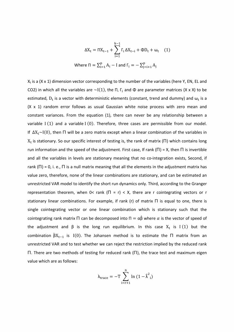
ΔX� � ΠX��� � � Γ���

��ΔX��� � ΦD� � ω� 1�

Where Π � ∑ A���� � I and Γ� � � ∑ A�

�����

Xt is a (X x 1) dimension vector corresponding to the number of the variables (here Y, EN, EL and

CO2) in which all the variables are ~I 1�, the Π, Γ� and Φ are parameter matrices (X x X) to be

estimated, D� is a vector with deterministic elements (constant, trend and dummy) and ω� is a

(X x 1) random error follows as usual Gaussian white noise process with zero mean and

constant variances. From the equation (1), there can never be any relationship between a

variable I 1� and a variable I 0�. Therefore, three cases are permissible from our model.

If ∆X�~I 0�, then Π will be a zero matrix except when a linear combination of the variables in

X� is stationary. So our specific interest of testing is, the rank of matrix (Π) which contains long

run information and the speed of the adjustment. First case, If rank (Π) = X, then Π is invertible

and all the variables in levels are stationary meaning that no co-integration exists, Second, if

rank (Π) = 0, i. e., Π is a null matrix meaning that all the elements in the adjustment matrix has

value zero, therefore, none of the linear combinations are stationary, and can be estimated an

unrestricted VAR model to identify the short run dynamics only. Third, according to the Granger

representation theorem, when 0< rank (Π = r) < X, there are r cointegrating vectors or r

stationary linear combinations. For example, if rank (r) of matrix Π is equal to one, there is

single cointegrating vector or one linear combination which is stationary such that the

cointegrating rank matrix Π can be decomposed into Π � αβ� where � is the vector of speed of

the adjustment and β is the long run equilibrium. In this case X� is I 1� but the

combination β� X��� is I 0�. The Johansen method is to estimate the Π matrix from an

unrestricted VAR and to test whether we can reject the restriction implied by the reduced rank

Π. There are two methods of testing for reduced rank (Π), the trace test and maximum eigen

value which are as follows:

�� ! � �T � ln 1 �%

����λ&'

��

λ(�) r, r � 1� � �Tln 1 � λ����

Where, +, is the estimated ordered eigenvalue obtained from the estimated matrix and T is the

number of usable observations after lag adjustment. The trace statistics tests the null

hypothesis that the number of distinct cointegrating vector (r) is less than or equal to r against a

general alternative. The maximal eigenvalue tests the null that the number of cointegrating

vector is r against the alternative of r +1 cointegrating vector.

Autoregressive distributed lag (ARDL) bound test for cointegration

In addition to the Johansen cointegration rank test, we also performed an ARDL model for

bound test introduced by the Pesaran et al., (2001). Although Gonzalo (1994) presents Monte

Carlo evidence that the full information maximum likelihood procedure of Johansen test

performs better than others and the test is appropriate when the identification of exogenous

variable is not possible at prior, but the Johansen test result is very sensitive in the case of small

sample and the use of different lag length (Odhiaambo, 2009). ARDL bound test has many

advantages over other cointegration tests in this regards. The ARDL does not impose any

restriction that all the variables used under study must be integrated of the same order;

therefore the test can be applied whether the selected variables are integrated of order zero or

order one. The test is also not sensitive to the size of the sample. Moreover, the ARDL test

generally provides unbiased estimates of the long run model and provides valid t-statistics even

when some of the regressors are endogenous (Harris and Sollis, 2003). Pesaran and Shin (1998)

show that it is possible to test the long run relationship between the dependent and the set of

regressors when it is not known a prior whether the variables are stationary or non-stationary.

Following Pesaran and Shin we have estimated the following equations to investigate the long

run level relationships which are as follows

∆X�,�μ� � � β�∆X�,��� �-�

��α�,X�,��� � ε�,� 2�

The equation 2 can be rewritten as

∆X�,�μ � � β�∆X�,��� �-�

��� β�∆X',��� �-'

��α�,X�,��� � α',X',����ε�,� 3�

∆X',�φ � � β�∆X�,��� �-�

��� β�∆X',��� �-'

��α�,X�,��� � α',X',����ε',� 4�

Here, all the variables are previously defined. The cointegration is examined based on F-

statistics. From the above equations 3 and 4, the presence of cointegration can be tested first

estimating the models by OLS and then by restricting all estimated coefficients of lagged level

variables equal to zero. So the null hypothesis H0: α1=α2=0 is tested against the alternative of

H1: α1 =≠ α2 ≠ 0. The number of lag was chosen based on likelihood ratio (LR) criteria. The

estimated F-test has a non-standard distribution, however. Two set of critical values are

provided for given significance level at Pesaron et al., (2001). First set of critical values assumes

that all the variables are I (0) and the second set assumes that the all variables are I (1). If the

calculated F-statistics exceeds the upper bounds of I (1), then the null of no cointegration is

rejected. If the estimated F-statistics is smaller than the lower bounds of I (0), then the null

hypothesis of no cointegration can’t be rejected. The test becomes inclusive if the calculated F-

statistics falls into the bounds.

Granger causality in the VECM framework

Once the cointegration relationship confirmed from the Johansen and the ARDL bound test, we

use the Granger causality in a Johansen vector error correction framework. The existence of

cointegration in the bi-variate relationship implies long run Granger causality at least one

direction which under certain restrictions can be tested Wald test (Masconi and Giannini 1992;

Dolado and Lutkephol, 1996). If α matrix in the cointegration rank matrix (Π) has a complete

column of zeros, no long run casual relationship exist, because there is no cointegrating vector

appear in that particular block. For identifying the short run and the long run causal

relationship, the equation (1) can be re-written in the case of bi-variate model as following two

equations

∆X�,�μ� � � β�∆X�,��� � � β�∆X',���'

���

�

��α�ECT ��� � ε�,� 5�

∆X',�μ' � � β�∆X�,��� � � β�∆X',���'

���

�

��α'ECT ��� � ε�,� 6�

Where, ECT stands for error correction term. In the equations (5 and 6), there are three

possible cases of testing long run causality. First; if α1 ≠0 and α2≠0, which implies bi-directional

causality that there exist a feed-back long run relationship between the selected variables. Two

variables cause each other in the long run. Second, if α1 =0 but α2 ≠0, implies unidirectional

causality meaning that variable X2 granger cause to variable X1. Third, if, α2=0 but α1 ≠0, implies

uni-directional causality, variable X1 granger cause to variable X2. There can never be both α1 =0,

α2=0 once there is a cointegration relationship exist. We also can test the short run causality

from the equations 5 and 6 by using standard Wald test. We can examine the significance of all

lagged dynamic terms by testing for example in equation 5, the null of Ho: β� � 0. Non-

rejection implies that variable X2 granger cause to variable X1 in the short run and the null of Ho:

β� � 0. in equation 6 implies that variable X1 granger cause to variable X2.

3. Empirical results and discussions

The results of ADF and PP tests on each of the variables are reported in Table 1. The results

indicate that all series are non-stationary at their level but stationary at their first differences

irrespective the random walk model with drift or random walk model with slope. In time series

econometrics, it is said that series are integrated of order one denoted by presenting X�~I 1�

and series of integrated of order zero denoted by ∆X�~I 0�. Here, the order of the integration

is one. Note that, the same order of integration is a pre-requisite when the Johansen

framework is used for testing cointegration and the causality. Our Johansen test is

complemented by the ARDL bound test. That is why we also have to check whether any of the

variables is I (2) because of the critical values provided by Pesaron et al., (2001) are only for I (0)

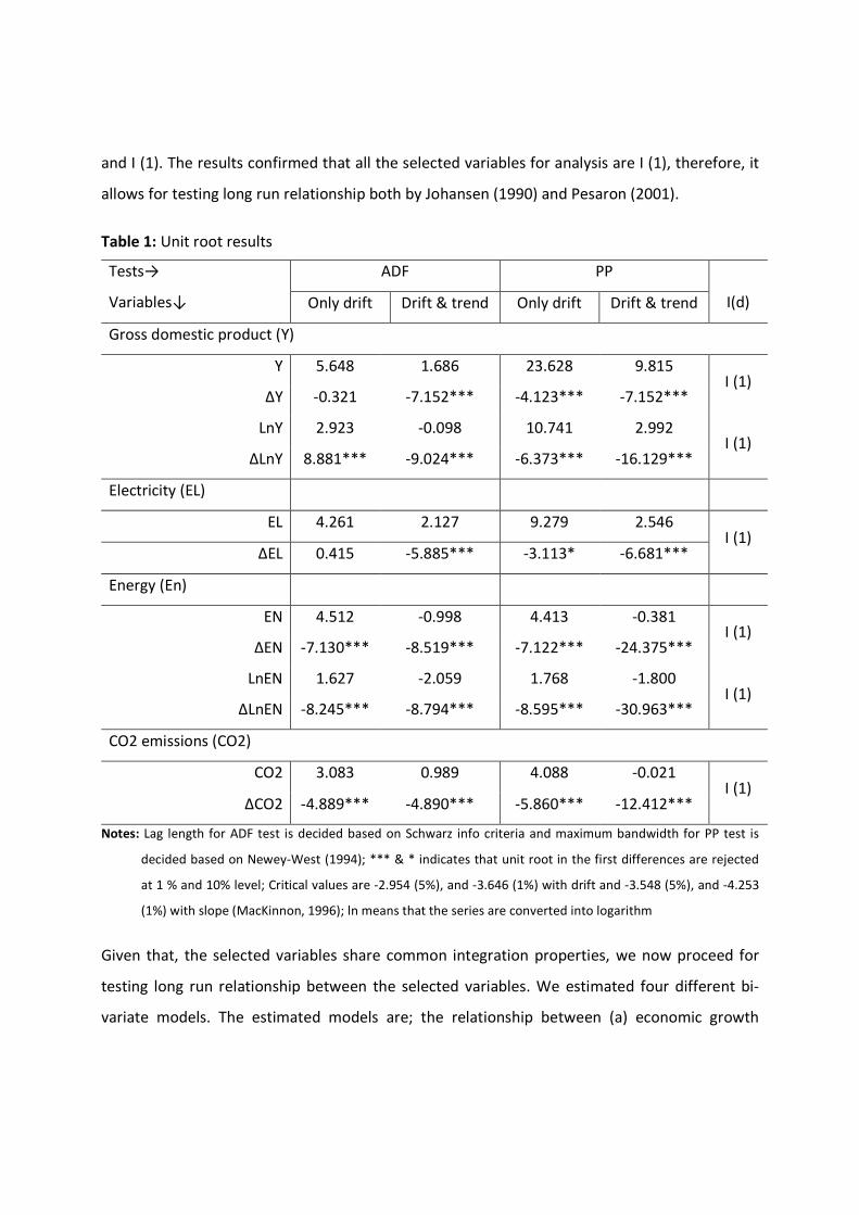
and I (1). The results confirmed that all the selected variables for analysis are I (1), therefore, it

allows for testing long run relationship both by Johansen (1990) and Pesaron (2001).

Table 1: Unit root results

Tests→

Variables↓

ADF PP

I(d) Only drift Drift & trend Only drift Drift & trend

Gross domestic product (Y)

Y 5.648 1.686 23.628 9.815 I (1)

∆Y -0.321 -7.152*** -4.123*** -7.152***

LnY 2.923 -0.098 10.741 2.992 I (1)

∆LnY 8.881*** -9.024*** -6.373*** -16.129***

Electricity (EL)

EL 4.261 2.127 9.279 2.546 I (1)

∆EL 0.415 -5.885*** -3.113* -6.681***

Energy (En)

EN 4.512 -0.998 4.413 -0.381 I (1)

∆EN -7.130*** -8.519*** -7.122*** -24.375***

LnEN 1.627 -2.059 1.768 -1.800 I (1)

∆LnEN -8.245*** -8.794*** -8.595*** -30.963***

CO2 emissions (CO2)

CO2 3.083 0.989 4.088 -0.021 I (1)

∆CO2 -4.889*** -4.890*** -5.860*** -12.412***

Notes: Lag length for ADF test is decided based on Schwarz info criteria and maximum bandwidth for PP test is

decided based on Newey-West (1994); *** & * indicates that unit root in the first differences are rejected

at 1 % and 10% level; Critical values are -2.954 (5%), and -3.646 (1%) with drift and -3.548 (5%), and -4.253

(1%) with slope (MacKinnon, 1996); ln means that the series are converted into logarithm

Given that, the selected variables share common integration properties, we now proceed for

testing long run relationship between the selected variables. We estimated four different bi-

variate models. The estimated models are; the relationship between (a) economic growth

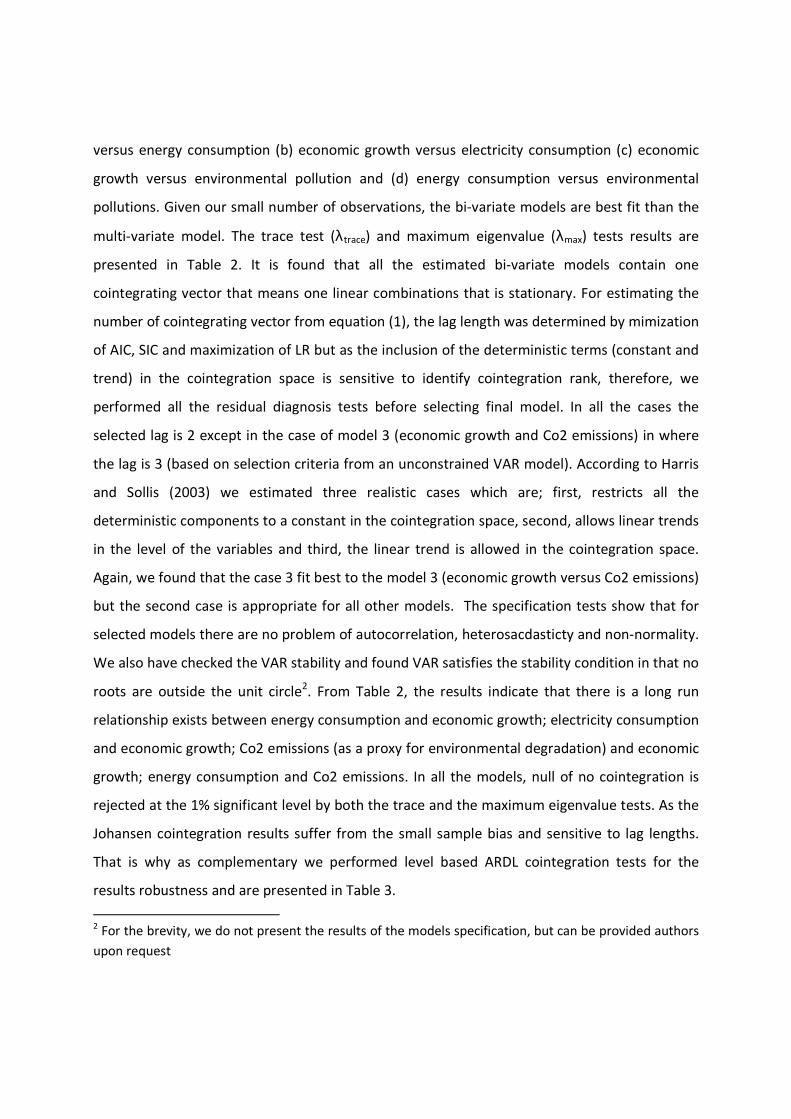
versus energy consumption (b) economic growth versus electricity consumption (c) economic

growth versus environmental pollution and (d) energy consumption versus environmental

pollutions. Given our small number of observations, the bi-variate models are best fit than the

multi-variate model. The trace test (λtrace) and maximum eigenvalue (λmax) tests results are

presented in Table 2. It is found that all the estimated bi-variate models contain one

cointegrating vector that means one linear combinations that is stationary. For estimating the

number of cointegrating vector from equation (1), the lag length was determined by mimization

of AIC, SIC and maximization of LR but as the inclusion of the deterministic terms (constant and

trend) in the cointegration space is sensitive to identify cointegration rank, therefore, we

performed all the residual diagnosis tests before selecting final model. In all the cases the

selected lag is 2 except in the case of model 3 (economic growth and Co2 emissions) in where

the lag is 3 (based on selection criteria from an unconstrained VAR model). According to Harris

and Sollis (2003) we estimated three realistic cases which are; first, restricts all the

deterministic components to a constant in the cointegration space, second, allows linear trends

in the level of the variables and third, the linear trend is allowed in the cointegration space.

Again, we found that the case 3 fit best to the model 3 (economic growth versus Co2 emissions)

but the second case is appropriate for all other models. The specification tests show that for

selected models there are no problem of autocorrelation, heterosacdasticty and non-normality.

We also have checked the VAR stability and found VAR satisfies the stability condition in that no

roots are outside the unit circle2. From Table 2, the results indicate that there is a long run

relationship exists between energy consumption and economic growth; electricity consumption

and economic growth; Co2 emissions (as a proxy for environmental degradation) and economic

growth; energy consumption and Co2 emissions. In all the models, null of no cointegration is

rejected at the 1% significant level by both the trace and the maximum eigenvalue tests. As the

Johansen cointegration results suffer from the small sample bias and sensitive to lag lengths.

That is why as complementary we performed level based ARDL cointegration tests for the

results robustness and are presented in Table 3.

2 For the brevity, we do not present the results of the models specification, but can be provided authors

upon request

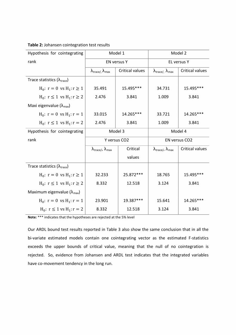
Table 2: Johansen cointegration test results

Hypothesis for cointegrating

rank

Model 1 Model 2

EN versus Y EL versus Y

λtrace/, λmax Critical values λtrace/, λmax Critical values

Trace statistics (λtrace)

H6: r � 0 vs H�: r : 1 35.491 15.495*** 34.731 15.495***

H6: r ; 1 vs H�: r : 2 2.476 3.841 1.009 3.841

Maxi eigenvalue (λmax)

H6: r � 0 vs H�: r � 1 33.015 14.265*** 33.721 14.265***

H6: r ; 1 vs H�: r � 2 2.476 3.841 1.009 3.841

Hypothesis for cointegrating

rank

Model 3 Model 4

Y versus CO2 EN versus CO2

λtrace/, λmax Critical

values

λtrace/, λmax Critical values

Trace statistics (λtrace)

H6: r � 0 vs H�: r : 1 32.233 25.872*** 18.765 15.495***

H6: r ; 1 vs H�: r : 2 8.332 12.518 3.124 3.841

Maximum eigenvalue (λmax)

H6: r � 0 vs H�: r � 1 23.901 19.387*** 15.641 14.265***

H6: r ; 1 vs H�: r � 2 8.332 12.518 3.124 3.841

Note: *** indicates that the hypotheses are rejected at the 5% level

Our ARDL bound test results reported in Table 3 also show the same conclusion that in all the

bi-variate estimated models contain one cointegrating vector as the estimated F-statistics

exceeds the upper bounds of critical value, meaning that the null of no cointegration is

rejected. So, evidence from Johansen and ARDL test indicates that the integrated variables

have co-movement tendency in the long run.

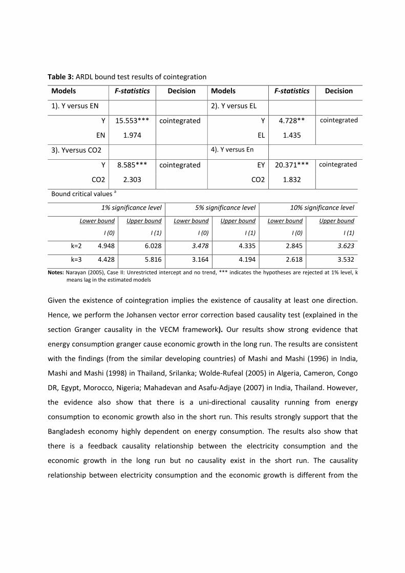
Table 3: ARDL bound test results of cointegration

Models F-statistics Decision Models F-statistics Decision

1). Y versus EN 2). Y versus EL

Y 15.553*** cointegrated Y 4.728** cointegrated

EN 1.974 EL 1.435

3). Yversus CO2 4). Y versus En

Y 8.585*** cointegrated EY 20.371*** cointegrated

CO2 2.303 CO2 1.832

Bound critical values a

1% significance level 5% significance level 10% significance level

Lower bound

I (0)

Upper bound

I (1)

Lower bound

I (0)

Upper bound

I (1)

Lower bound

I (0)

Upper bound

I (1)

k=2 4.948 6.028 3.478 4.335 2.845 3.623

k=3 4.428 5.816 3.164 4.194 2.618 3.532

Notes: Narayan (2005), Case II: Unrestricted intercept and no trend, *** indicates the hypotheses are rejected at 1% level, k

means lag in the estimated models

Given the existence of cointegration implies the existence of causality at least one direction.

Hence, we perform the Johansen vector error correction based causality test (explained in the

section Granger causality in the VECM framework). Our results show strong evidence that

energy consumption granger cause economic growth in the long run. The results are consistent

with the findings (from the similar developing countries) of Mashi and Mashi (1996) in India,

Mashi and Mashi (1998) in Thailand, Srilanka; Wolde-Rufeal (2005) in Algeria, Cameron, Congo

DR, Egypt, Morocco, Nigeria; Mahadevan and Asafu-Adjaye (2007) in India, Thailand. However,

the evidence also show that there is a uni-directional causality running from energy

consumption to economic growth also in the short run. This results strongly support that the

Bangladesh economy highly dependent on energy consumption. The results also show that

there is a feedback causality relationship between the electricity consumption and the

economic growth in the long run but no causality exist in the short run. The causality

relationship between electricity consumption and the economic growth is different from the

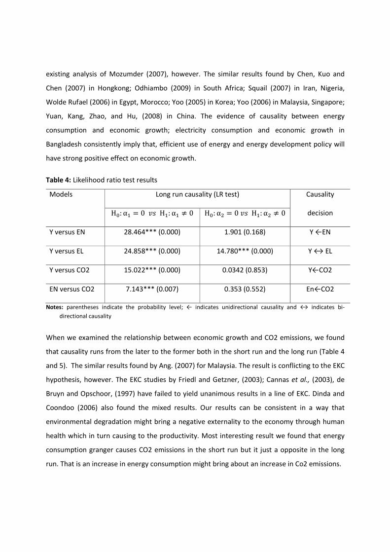
existing analysis of Mozumder (2007), however. The similar results found by Chen, Kuo and

Chen (2007) in Hongkong; Odhiambo (2009) in South Africa; Squail (2007) in Iran, Nigeria,

Wolde Rufael (2006) in Egypt, Morocco; Yoo (2005) in Korea; Yoo (2006) in Malaysia, Singapore;

Yuan, Kang, Zhao, and Hu, (2008) in China. The evidence of causality between energy

consumption and economic growth; electricity consumption and economic growth in

Bangladesh consistently imply that, efficient use of energy and energy development policy will

have strong positive effect on economic growth.

Table 4: Likelihood ratio test results

Models Long run causality (LR test) Causality

decision H6: α� � 0 => H�: α� ? 0 H6: α' � 0 => H�: α' ? 0

Y versus EN 28.464*** (0.000) 1.901 (0.168) Y ←EN

Y versus EL 24.858*** (0.000) 14.780*** (0.000) Y ↔ EL

Y versus CO2 15.022*** (0.000) 0.0342 (0.853) Y←CO2

EN versus CO2 7.143*** (0.007) 0.353 (0.552) En←CO2

Notes: parentheses indicate the probability level; ← indicates unidirectional causality and ↔ indicates bi-

directional causality

When we examined the relationship between economic growth and CO2 emissions, we found

that causality runs from the later to the former both in the short run and the long run (Table 4

and 5). The similar results found by Ang. (2007) for Malaysia. The result is conflicting to the EKC

hypothesis, however. The EKC studies by Friedl and Getzner, (2003); Cannas et al., (2003), de

Bruyn and Opschoor, (1997) have failed to yield unanimous results in a line of EKC. Dinda and

Coondoo (2006) also found the mixed results. Our results can be consistent in a way that

environmental degradation might bring a negative externality to the economy through human

health which in turn causing to the productivity. Most interesting result we found that energy

consumption granger causes CO2 emissions in the short run but it just a opposite in the long

run. That is an increase in energy consumption might bring about an increase in Co2 emissions.

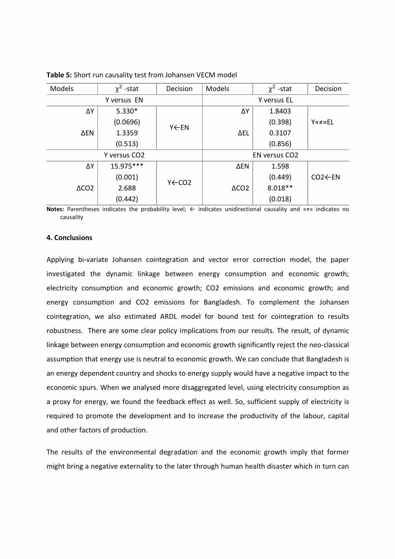
Table 5: Short run causality test from Johansen VECM model

Models χ' -stat Decision Models χ' -stat Decision

Y versus EN Y versus EL

∆Y 5.330*

(0.0696) Y←EN

∆Y 1.8403

(0.398)

Y«≠»EL

∆EN 1.3359

(0.513)

∆EL 0.3107

(0.856)

Y versus CO2 EN versus CO2

∆Y 15.975***

(0.001) Y←CO2

∆EN 1.598

(0.449)

CO2←EN

∆CO2 2.688

(0.442)

∆CO2 8.018**

(0.018)

Notes: Parentheses indicates the probability level; ← indicates unidirectional causality and «≠» indicates no

causality

4. Conclusions

Applying bi-variate Johansen cointegration and vector error correction model, the paper

investigated the dynamic linkage between energy consumption and economic growth;

electricity consumption and economic growth; CO2 emissions and economic growth; and

energy consumption and CO2 emissions for Bangladesh. To complement the Johansen

cointegration, we also estimated ARDL model for bound test for cointegration to results

robustness. There are some clear policy implications from our results. The result, of dynamic

linkage between energy consumption and economic growth significantly reject the neo-classical

assumption that energy use is neutral to economic growth. We can conclude that Bangladesh is

an energy dependent country and shocks to energy supply would have a negative impact to the

economic spurs. When we analysed more disaggregated level, using electricity consumption as

a proxy for energy, we found the feedback effect as well. So, sufficient supply of electricity is

required to promote the development and to increase the productivity of the labour, capital

and other factors of production.

The results of the environmental degradation and the economic growth imply that former

might bring a negative externality to the later through human health disaster which in turn can

cause to the poor productivity. This is consistent with the experiences of many developing

countries, however. Therefore, the policy makers have to make strategic plans so that the

environmental quality is not persistently decline which will have negative externality to output

growth.

References

Ang, J. B. (2007). Co2 emissions, energy consumption, and output in France. Energy Policy, 35,

4772–4778

Asafu-A. J., (2000). The relationship between energy consumption, energy prices and economic

growth: time series evidence from Asian developing countries. Energy Economics, 22,

615-625

BBS (2005). Statistical Yearbook of Bangladesh. the ministry of planning, the Peoples Republic

of the Government of Bangladesh

Canas, A., Ferrao, P., Conceicao, P., (2003). A new environmental Kuznets curve? Relationship

between direct material input and income per capita: evidence from industrialized

countries. Ecological Economics, 46, 217-229

Chen S. T., Kuo H. I, Chen C. C. (2007). The relationship between GDP and electricity

consumption in 10 Asian countries. Energy Policy, 35, 2611–2621

Cheng, B. S. (1998). Energy consumption, employment and causality in Japan: a multivariate

approach. Indian Economic Review, 33, 19-29

Chontanawat, J., Hunt, L. C. and Pierse, R., (2008). Does energy consumption cause economic

growth? Evidence from a systematic study of over 100 countries, Journal of Policy

Modeling, 30, 209-220

Chontanawat, J., Hunt, L.C. and Pierse, R., (2006). Causality between energy consumption and

GDP: evidence from 30 OECD and 78 non-OECD countries. Surrey energy economics

discussion paper series 113, University of Surrey, Guildford

de Bruyn, S.M., Opschoor, J.B., (1997). Developments in the throughput-income relationship:

theoretical and empirical observations. Ecological Economics, 20, 255–268

Dickey, D., Fuller, W., (1979). Distribution of the estimators for autoregressive time series with

a unit root. Journal of American Statistical Associations, 74, 427-431

Dinda, S. (2004). Environmental Kuznets curve hypothesis: A survey. Ecological Economics, 49,

431–455

Dinda, S., Coondoo, D., (2006). Income and emission: a panel-data based cointegration analysis.

Ecological Economics, 57, 167–181

Dolado, J., and Lutkepohl, H., S., (1996). Making Wald tests for cointegrated VAR systems.

Econometric Reviews, 15(4), 369-386

Elif, A., S., Turut-A., Ipek, T., (2009). The relationship between income and environment in

Turkey: Is there an environmental Kuznets Curve? Energy policy, 37, 861-867

Engle, R. F. and Granger, C. W., (1987). Cointegration and error correction: representation,

estimation and testing, Econometrica, 55, 251-276

Friedl, B., Getzner, M., (2003). Determinants of Co2 emissions in a small open economy.

Ecological Economics, 45, 133–148

Gonzalo, J., (1994). Five alternative methods of estimating long run equilibrium relationship.

Journal of Econometrics, 60, 203-233.

Grossman, G.M., Krueger, A. B. (1991). Environmental impact of a North American Free Trade

Agreement. Working Paper 3914, National Bureau of Economic Research, Cambridge, M.

A

Harris, R., & Sollis, R., (2003). Applied Time Series Modeling and Forecasting. Chichester: John

Wiley and Sons Ltd.

IPCC, Climate Change (2001). The scientific basis, 2001, Cambridge; Cambridge press

Johansen, S., Juselius, K., (1990). Maximum likelihood estimation and inference on

cointegration- with applications to the demand for money. Oxford Bulletin of Economics

and Statistics, 52 (2), 169–210

Kraft, J., Kraft, A. (1978). On the relationship between energy and GNP. Journal of Energy

Development 3, 401-413

Kuznets, S., (1955). Economic growth and income inequality. American Economic Reviews, 17,

57-84

MacKinnon, J. G., (1996). Numerical distribution functions for unit root and cointegration tests,

Journal of Applied Econometrics, 11, 601-618

Mahadevan, R. and Asafu-A , J., (2007). Energy consumption, economic growth and prices: a

reassessment using panel VECM for developed and developing countries. Energy Policy,

35, 2481-90

Masih, A. M. M. and Masih, R., (1996). Energy consumption, real income and temporal

causality: results from a multi-country study based on cointegration and error-

correction modeling techniques. Energy Economics, 18, 165-183

Masih, A. M. M. and Masih, R., (1998). A Multivariate cointegrated modeling approach in

testing temporal causality between energy consumption, real income, and prices with

an application to two Asian LDCs. Applied Economics, 30, 1287-1298

Mosconi R, and Giannini, C., (1992). Non-causality in cointegrated systems: representation,

estimation and testing. Oxford Bulletin of Economics and Statistics 54: 399–417

Mozumder, P., Marathe, A. (2007). Causality relationship between electricity consumption and

the GDP in Bangladesh. Energy Policy, 35, 395-402

Narayan, P. K., (2005). The savings and investment nexus for China: evidence from

cointegration test. Applied Economics, 1979-1980.

Newey, W. and West, K., (1994). Automatic lag selection in covariance matrix estimation.

Review of Economic Studies, 61, 631-653

Odhiambo, N. M (2009a). Electricity consumption and the economic growth in South Africa: a

tri-variate causality test. Energy Economics, 31 (5), 635

Odhiambo, N. M., (2009b). Energy consumption and economic growth nexus in Tanzania: An

ARDL bounds testing approach. Energy Policy, 37, 617-622

Payne, J. E., (2010a). Survey of the international evidence on the causal relationship between

energy consumption and growth. Journal of Economic Studies, 37, 53-95

Payne, J. E., (2010b). A Survey of the electricity consumption-growth literature. Applied

Energy,87, 723-731

Pesaran, M. H., and Shin, Y., (1998). An autoregressive distributed lag modeling approach to

cointegration analysis. In: Strom, S., Diamond, P., (Eds.), Centennial Volume of Regnar

Frisch. Cambridge University Press, Cambridge

Pesaran, M., Shin, and Y., Smith, R., (2001). Bounds testing approaches to the analysis of level

relationship. Journal of Applied Econometrics, 16, 289-326

Phillips, P. C. B., and Perron, P., (1988). Testing for a unit root in time series regression.

Biometrika, 75 (2), 336-346

Selden, T. M., and Song, D., (1994). Environmental quality and development: Is there a Kuznets

curve for air pollution? Journal of Environmental Economics and Management, 27, 147-

162

Six-Five Year Plan, 2010 (Forthcoming). The planning commission, the ministry of planning, the

People’s Republic of the Government of Bangladesh

Soytas, U. and Sari, R. (2007). Energy consumption, economic growth, and carbon emissions:

challenges faced by an EU candidate member. Ecological Economics, 68, 1667-1675

Soytas, U. and Sari, R., (2003). Energy consumption and GDP: causality relationship in G-7 and

emerging markets. Energy Economics, 25, 33-7

Squalli, J., (2007). Electricity consumption and economic growth: bounds and causality analyses

of OPEC countries. Energy Economics, 29, 1192–1205

Stern, D. I., (1993). Energy and economic growth in the USA: a multivariate approach. Energy

Economics, 15, 137-150

Stern, D. I., (2000). A multivariate cointegration analysis of the role of energy in the US

macroeconomy. Energy Economics, 22, 267-83.

Stern, D. I., Common, M. S., & Barbier, E. B., (1996). Economic growth and environmental

degradation: A critique of the environmental Kuznets curve. World Development, 24 (7),

1151-1160

Toda, H. Y., Yamamoto, T., (1995). Statistical inference in vector auto regression with possibly

integrated process. Journal of Econometrics, 66, 225-250

Wolde-Rufael Y., (2006). Electricity consumption and economic growth: a time series

experience for 17 African countries. Energy Policy, 34, 1106–1114

Wolde-Rufael, Y., (2004). Disaggregated industrial energy consumption and GDP: the case of

Shanghai, 1952-1999. Energy Economics, 26, 69-75

Wolde-Rufael, Y., (2005). Energy demand and economic growth: the African experience. Journal

of Policy Modeling, 27, 891-903

World Bank (2010). World Development Indicators 2010 (CD-ROM), IBRD, World Bank,

Washington D.C

Yoo, S. H., (2005). Electricity consumption and economic growth: evidence from Korea. Energy

Policy, 33, 1627–1632

Yoo, S. H., (2006). The causal relationship between electricity consumption and economic

growth in the ASEAN countries. Energy Policy, 34, 3573–3578

Yuan J., Zhao C., Yu S., and Hu, Z., (2007). Electricity consumption and economic growth in

China: cointegration and co-feature analysis. Energy Economics, 29, 1179–1191