Energy & Commodity Markets I

Ronnie Sircar

Department of Operations Research and Financial Engineering

Princeton University

http://www.princeton.edu/∼sircar

1

Overview

1. Traditional commodity markets issues and models. Electricity

price models.

2. Energy production from exhaustible resources and renewables:

game threoretic models.

3. Financialization of commodity markets.

2

Commodity Forward Curves

◮ By commodities, we refer to◮ Agriculturals: (soybeans, corn, coffee, sugar, ...)◮ Metals (copper, aluminum, gold, silver, ...)◮ Energy (oil, natural gas, coal, power, carbon, ...)◮ Livestock (live cattle, frozen pork bellies, ...),◮ Shipping / Freight, Weather (temperature, rainfall)

◮ They are widely traded on standardised exchanges such as the

Chicago Board of Trade (CBOT), the London Metal Exchange

(LME), New York Mercantile Exchange (NYMEX).

◮ Idealized notion: spot price (St), akin to stock price. But

storability is a major distinction.

◮ The basic financial instrument is the forward, with the forward

price F(t,T) being the price agree today (time t) for delivery on

maturity date T , and so

limt→T

F(t,T) = ST .

3

Forward Prices when no Storage Cost

◮ Portfolio A: Long forward at time t

◮ Time t: costs nothing to enter forward contract;◮ Time T: portfolio realizes ST − F(t, T).

◮ Portfolio B: Buy spot, borrow $x

◮ Time t: costs St − x;◮ Time T: portfolio realizes ST − xer(T−t).

◮ Choose x = Fe−r(T−t), then portfolios A and B have identical

payoffs.

◮ No arbitrage implies the must cost the same to enter, so

0 = St − x ⇒ F(t,T) = Ster(T−t).

◮ But the ‘buy spot’ side of the arbitrage cannot easily be executed

when the commodity has to be stored. Leads to modifications

described as cost of carry and convenience yield.

4

Backwardation & Contango

◮ Upward sloping forward curve: contango .

◮ Downward sloping: backwardation .

◮ Historically, forward curves have been in backwardation about

75% of the time. But in contango more often more recently.

◮ Keynes’ theory of backwardation (1930s): F(t,T) should be a

downward biased estimate of ST , i.e. spot should be greater than

forward prices.

◮ Explained by the hedging pressure on commodity producers:

◮ Producers : long commodity, sell forwards to hedge;◮ Consumers : short commodity, buy forwards to hedge.

◮ Keynes: producers dominate due to fragmentation of consumers.

They pay a premium to lock in prices.

◮ More recent contango (oil): pushed up by speculators?

Financialization.

5

Convenience Yield

◮ Typical modification to forward prices:

F(t,T) = Ste(r+c−δ)(T−t),

where the (vague) variables are:

◮ c is cost of carry: rent for storage;◮ δ is convenience yield: benefits holder of spot, but not the holder

of the forward, inversely related to inventory levels.

◮ Large δ: backwardation.

◮ Small δ, large c: contango.

◮ Making c, δ time-varying and random: can switch between

backwardation and contango.

6

Spot Price Models

◮ Under a risk-neutral measure Q, spot is GBM:

dSt

St

= (r − δ) dt + σ dWQt .

◮ No arbitrage arguments dictate that

F(t,T) = IEQ{ST | St} = e(r−δ)(T−t)St.

◮ Leads todF(t,T)

F(t,T)= σ dW

Qt .

Volatility of forward is constant and independent of T .

◮ Samuelson effect: volatility is greater for shorter maturity

forwards.

◮ Captured by mean-reverting spot price models.

7

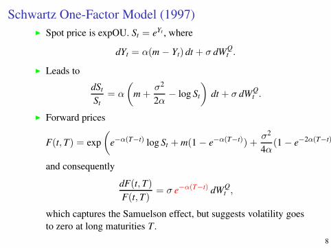
Schwartz One-Factor Model (1997)

◮ Spot price is expOU. St = eYt , where

dYt = α(m − Yt) dt + σ dWQt .

◮ Leads to

dSt

St

= α

(

m +σ2

2α− log St

)

dt + σ dWQt .

◮ Forward prices

F(t,T) = exp

(

e−α(T−t) log St + m(1 − e−α(T−t)) +σ2

4α(1 − e−2α(T−t)

and consequently

dF(t,T)

F(t,T)= σ e−α(T−t) dW

Qt ,

which captures the Samuelson effect, but suggests volatility goes

to zero at long maturities T .

8

Other Limitations

◮ Limited range of forward curve shapes.

◮ With one α, misprice either the long or the short end.

◮ Perfect correlation between front and back end of forward curve.

Both must move in sync, but not observed to do so empirically.

◮ Leads naturally to multi-factor models, e.g. Schwartz two-factor

model:

dSt

St

= (r − δt) dt + σ1 dWQt

dδt = α(µ − δt) dt + σ2 dBQt .

◮ Also Schwartz & Smith (2000); Schwartz 3-factor which has

stochastic (Vasicek) interest rate.

9

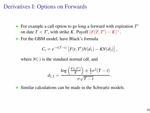
Derivatives I: Options on Forwards

◮ For example a call option to go long a forward with expiration T ′

on date T < T ′, with strike K. Payoff (F(T,T ′)− K)+.

◮ For the GBM model, have Black’s formula

Ct = e−r(T−t)[

F(t,T ′)N(d1)− KN(d2)]

,

where N(·) is the standard normal cdf, and

d1,2 =log(

F(t,T′)K

)

± 12σ2(T − t)

σ√

T − t.

◮ Similar calculations can be made in the Schwartz models.

10

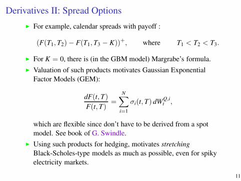
Derivatives II: Spread Options

◮ For example, calendar spreads with payoff :

(F(T1,T2)− F(T1,T3 − K))+, where T1 < T2 < T3.

◮ For K = 0, there is (in the GBM model) Margrabe’s formula.

◮ Valuation of such products motivates Gaussian Exponential

Factor Models (GEM):

dF(t,T)

F(t,T)=

N∑

i=1

σi(t,T) dWQ,it ,

which are flexible since don’t have to be derived from a spot

model. See book of G. Swindle.

◮ Using such products for hedging, motivates stretching

Black-Scholes-type models as much as possible, even for spiky

electricity markets.

11

A Model for Hedging Load and Price Risk in the Texas

Electricity Market (Coulon, Powell, Sircar 2013)

◮ Use of financial products, e.g. futures and options, by retail

suppliers to hedge electricity price and demand spikes has grown

recently.

◮ As well as spikes, power prices have strong seasonal

components, are linked to fuel prices (esp. natural gas), driven

by demand (or load), and depend on transmission capacity.

◮ Typical in financial options problems to use continuous time

stochastic models built on Brownian motion. Here we want to try

and capture the above features, even spikes, with diffusions.

◮ Motivated by convenient pricing formulas which can reduce the

simulation burden on an optimization program for hedging risk.

12

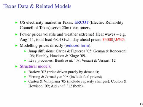
Texas Data & Related Models

◮ US electricity market in Texas: ERCOT (Electric Reliability

Council of Texas) serve 20m+ customers.

◮ Power prices volatile and weather extreme! Heat waves – e.g.

Aug ’11, total load 68.4 Gwh, day ahead prices $3000/MWh.

◮ Modelling prices directly (reduced form):

◮ Jump diffusions: Cartea & Figueroa ’05; Geman & Roncoroni

’06; Hambly, Howison & Kluge ’09.◮ Lévy processes: Benth et al. ’08; Veraart & Veraart ’12.

◮ Structural models:

◮ Barlow ’02 (price driven purely by demand);◮ Pirrong & Jermakyan ’08 (include fuel prices);◮ Cartea & Villaplana ’05 (include capacity changes); Coulon &

Howison ’09; Aid et al. ’12 (both).

13

!"

#!"

$!"

%!"

&!"

'!"

(!")*+,!'"

)-.,!'"

)*+,!("

)-.,!("

)*+,!/"

)-.,!/"

)*+,!0"

)-.,!0"

)*+,!1"

)-.,!1"

)*+,#!"

)-.,#!"

)*+,##"

)-.,##"

23456"7*8.9":;<=*><"?@*A"BCDEFG"

(a) Historical daily average ERCOT loads

!"

#"

$!"

$#"

%!"

%#"

&!"

!"

#!"

$!!"

$#!"

%!!"

%#!"

&!!"

'()*!#"

'+,*!#"

'()*!-"

'+,*!-"

'()*!."

'+,*!."

'()*!/"

'+,*!/"

'()*!0"

'+,*!0"

'()*$!"

'+,*$!"

'()*$$"

'+,*$$"

1(2"34567"89:;

<=>?"

@AB74"34567"89:C

DE?"

@AB74"8FGHI="J(5,K"(LM?"

N(O+4(,"1(2"8P7)4K"P+Q?"

(b) Historical daily average electricity and

gas prices

Figure: ERCOT load and electricity prices over 2005-11, and natural gas

prices. Seasonality in loads and spikes in prices are clear.

14

Building the Model I

◮ First de-seasonalize the ERCOT load Lt:

Lt = S(t) + Lt,

where the seasonal component (estimated using hourly data) is

given by

S(t) = a1 + a2 cos(2πt + a3) + a4 cos(4πt + a5) + a6t + a71we.

Here a2(h) to a5(h) are the seasonal components, a6(h) picks up

the upward trend , and a7(h) captures the drop in demand on

weekends, and h is the hour;

◮ Then fit the residual load Lt to an Ornstein-Uhlenbeck (OU)

model:

dLt = −κLLt dt + ηL dW(L)t .

◮ Relation to natural gas priceGt, model as expOU:

d log Gt = κG(mG − log Gt) dt + ηG dW(G)t ,

where W(L) and W(G) are independent.

15

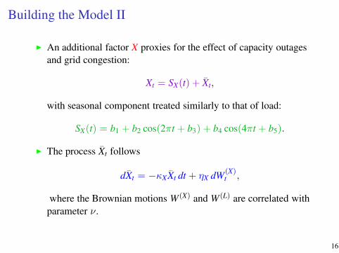
Building the Model II

◮ An additional factor X proxies for the effect of capacity outages

and grid congestion:

Xt = SX(t) + Xt,

with seasonal component treated similarly to that of load:

SX(t) = b1 + b2 cos(2πt + b3) + b4 cos(4πt + b5).

◮ The process Xt follows

dXt = −κXXt dt + ηX dW(X)t ,

where the Brownian motions W(X) and W(L) are correlated with

parameter ν.

16

Spike Mechanism

◮ The price Pt can spike in any hour as follows:

Pt = Gt exp(αmk+ βmk

Lt + γmkXt) for tk ≤ t < tk+1, k ∈ N.

◮ At each hour tk, the value of mk ∈ {1, 2} is determined by an

independent coin flip whose probabilities depend on the current

load Ltk :

mk =

1 with probability 1 − psΦ(

Ltk−µs

σs

)

2 with probability psΦ(

Ltk−µs

σs

)

,

where Φ(·) is the standard normal cdf.

◮ The choice of α2, β2, γ2 ( the spike regime) allows for a steeper

and potentially more volatile price to load relationship.

◮ Model for price is a mixture of lognormals: convenient for the

pricing of forwards and options.

17

Data & Fits

!"#

$"#

%"#

&"#

'"#

(!"#

!)!*# !)$# !)+*# !)*# !)&*# !)'# !),*#

-./01023245#/6#7892:;<#

=>1?@3;#/6#A;B1?C#

(a) Probability of spike vs load

!"

#"

$"

%"

&"

'"

("

!))))" #))))" $))))" %))))" &))))" '))))"

*+,"-./01"234"

516789"2:;<4"

!))("

!)=="

(b) Hourly price vs load for 2008 and 2011

Figure: Relationship between power price and load (right), and between

spike probability and load (left).

18

2 2.5 3 3.5 4 4.5 5 5.5 6 6.5

x 104

−10

0

10

20

30

40

50

60

70

80

90

100

load

pow

er /

gas

pric

e ra

tio

datamean of fitted curves (X=0)1 standard deviation (X=±1)

Figure: Fitting result - solid lines illustrate exponential price-load

relationship when X = 0 (at the mean), while dotted lines represent one

standard deviation bands (X = ±1).

19

Fitting to Data

◮ Primarily, use Maximum Likelihood Estimation after

deseasonalization.

◮ Find that the factors move on very different time scales: gas very

slowly mean-reverting over months (κG = 1.07); load mean

reverting over several days (κL = 92.6) and Xt mean reverting on

an intra-day time scale (κX = 1517).

◮ Find that ps = 0.129 implies that we visit the spike regime

approximately 6.5% of the time on average

◮ 6.11 × 10−5 = β2 > β1 = 2.79 × 10−5 so that in the spike

regime the exponential relationship between price and load is

significantly steeper, as expected in order to produce extreme

spikes.

◮ Moreover, 0.741 = γ2 > γ1 = 0.237, as the spike regime is also

more volatile than the normal price regime.

20

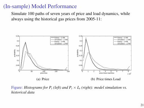
(In-sample) Model Performance

Simulate 100 paths of seven years of price and load dynamics, while

always using the historical gas prices from 2005-11:

0 50 100 150 2000

0.05

0.1

0.15

0.2

0.25

0.3

0.35

price bins

prob

abili

ty

history − 2 AMsimulation − 2 AMhistory − 2 PMsimulation − 2 PM

(a) Price

0 1 2 3 4 5 6 7 8

x 106

0

0.05

0.1

0.15

0.2

0.25

0.3

0.35

price times load bins

prob

abili

ty

history − 2 AMsimulation − 2 AMhistory − 2 PMsimulation − 2 PM

(b) Price times Load

Figure: Histograms for Pt (left) and Pt × Lt (right): model simulation vs.

historical data

21

A little known option pricing result from the 70’s

V0 = S0Φ2

(

h + σ√

T1, k + σ√

T2;

√

T1

T2

)

− K2e−rT2Φ2

(

h, k;

√

T1

T2

)

− Ke−rT1 Φ(h),

where h =log(S0/S∗)+(r− 1

2σ2)T1

σ√

T1, k =

log(S0/K)+(r− 12σ2)T2

σ√

T2and S∗ = . . .

◮ That was Geske’s 1977 result for compound options (a call on a call):

V0 = e−rT1EQ

[

(

CBST1(T2,K2)− K1

)+]

◮ It follows from the following very useful result:

∫ h

−∞ecxΦ

(

a + bx

d

)

e−12

x2

√2π

dx = e12

c2

Φ2

(

h − c,a + bc

√b2 + d2

;−b

√b2 + d2

)

where a, b, c, d, h are constants, and Φ(·),Φ2(·, ·; ρ) the Gaussian cdf’s.

◮ Interestingly, this same result proves valuable for energy derivatives...

22

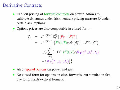
Derivative Contracts

◮ Explicit pricing of forward contracts on power. Allows to

calibrate dynamics under (risk-neutral) pricing measure Q under

certain assumptions.

◮ Options prices are also computable in closed-form:

Vpt = e−r(T−t)E

Qt

[

(PT − K)+]

= e−r(T−t){

Fg(t,T)c1Φ(

d+1

)

− KΦ(

d−1

)

+ps

2∑

i=1

(−1)i[

Fg(t,T)ciΦ2

(

d+i , g+i ;λi

)

−KΦ2

(

d−i , g−i ;λi

)]}

◮ Also: spread options on power and gas.

◮ No closed form for options on elec. forwards, but simulation fast

due to forwards explicit formula.

23

Revenue Hedging

◮ Consider here the case of a retail power utility company which

faces the choice of waiting and buying the required amount of

electricity each hour from the spot market, or hedging its

obligations in advance through the purchase of forwards, options

or some combination of the two.

◮ Simplified: we make a single hedging decision today. This is a

static hedge, so we do not (yet) consider dynamically re-hedging

through time.

◮ Setting τ = 1/365 and pfixed to be the price it charges its

customers per MWh, the firm’s revenue RT over the one-day

period [T,T + τ ] in the future is given by

RT =24∑

j=1

LTj

(

pfixed − PTj

)

, where Tj = T +j

24τ.

24

Hedging InstrumentsWe allow trading in the following contracts in order to hedge the

firm’s risk:

◮ Forward contracts with delivery on a particular hour j, with price

Fp(t,Tj)

◮ Call options on these forwards, with payoff at Tj − τ of

VpTj−τ = (Fp(Tj − τ,Tj)− K(j))+

◮ Spark spread options on forwards, with payoff

Vp,gTj−τ = (Fp(Tj − τ,Tj)− hFg(Tj − τ,Tj))

+

◮ Call options on the hourly spot power price, with payoff

VpTj=(

PTj− K(j)

)+

◮ Spark spread options on spot energy prices, with payoff

Vp,gTj

=(

PTj− hGTj

)+,

where h and K(j) are the heat rates and strikes specified in the option

contracts. We allow the hourly strikes to vary due to the large price

variation through the day, and in the base case consider only

at-the-money (ATM) options for all hours.25

Variance Reduction by Hedging

◮ Minimize

Var

(

RT −N∑

n=1

θnU(n)T

)

where the θ1, . . . , θN represent the quantities purchased of N

available hedging products with payoffs U(1)T , . . . ,U

(N)T .

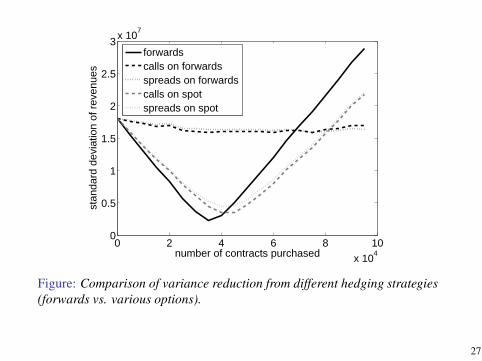
◮ First choose N = 1 to compare products one by one. See the

substantial benefit obtained from using derivative products to

hedge risk. Can clearly observe an optimal hedge quantity .

◮ When taken alone forward contracts are the most effective at

variance reduction. The next most effective hedge is options on

spot power.

◮ Spread options on spot power and gas provide slightly less

variance reduction, since they essentially isolate and hedge only

the risk of Lt and Xt, not the natural gas risk.

26

0 2 4 6 8 10

x 104

0

0.5

1

1.5

2

2.5

3x 10

7

number of contracts purchased

stan

dard

dev

iatio

n of

rev

enue

s

forwardscalls on forwardsspreads on forwardscalls on spotspreads on spot

Figure: Comparison of variance reduction from different hedging strategies

(forwards vs. various options).

27

Several Hedging Instruments

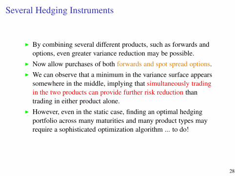
◮ By combining several different products, such as forwards and

options, even greater variance reduction may be possible.

◮ Now allow purchases of both forwards and spot spread options.

◮ We can observe that a minimum in the variance surface appears

somewhere in the middle, implying that simultaneously trading

in the two products can provide further risk reduction than

trading in either product alone.

◮ However, even in the static case, finding an optimal hedging

portfolio across many maturities and many product types may

require a sophisticated optimization algorithm ... to do!

28

01

2

x 104

2.533.54

x 104

1

2

3

4

5

6

7

8

9

10

x 106

number of optionsnumber of forwards

stan

dard

dev

iatio

n of

pro

fits

(a) Surface plot

2.5

2.5

2.5

2.5

3

3

3

3

3

3

3.5

3.5

3.5

3.5

3.5

3.5

3.5

3.5

4

4

4

4

4

4

4

4.5

4.5

4.5

4.5

4.5

5

5

5

5

5

5.5

5.5

5.5

6

6

6

6.5

6.5

7

7

7.5

8

num

ber

of fo

rwar

ds

number of options0 2000 4000 6000 8000 10000 12000 14000 16000 18000

2.4

2.6

2.8

3

3.2

3.4

3.6

3.8

4x 10

4

(b) Contour plot (all contour labels ×106)

Figure: Variance reduction when trading in both options and forwards.

29