ELSEVIER

CoastalEngineeringAll1a tI_.1 "_maI f... C.......

aM 0" ........

Coastal Engineering 43 (200!) 131-148

www.elsevier.com/locate/coastaleng

Energy balance of wind waves as a function of thebottom friction formulation

R. Padilla-Hemandez *, J. MonbaliuHydraulics Laboratory, Katholieke Universiteit Leuven, Kasteelpark Arenberg 40, B-3001 Heverlee. Belgium

Received 4 September 2000; received in revised fonn 14 February 2001; accepted 15 March 2001

Abstract

Four different expressions for wave energy dissipation by bottom friction are intercompared. For this purpose, the SWANwave model and the wave data set of Lake George (Australia) are used. Three formulations are already present in SWAN(ver. 40.00: the JONSWAP expression, the drag law friction model of Collins and the eddy-viscosity model of Madsen.The eddy-viscosity model of Weber was incorporated into the SWAN code. Using Collins' and Weber's expressions, thedepth- and fetch-limited wave growth laws obtained in the nearly idealized situation of Lake George can be reproduced. Thewave model has shown the best performance using the formulation of Weber. This formula has some advantages over theother formulations. The expression is based on theoretical and physical principles. The wave height and the peak frequencyobtained from the SWAN runs using Weber's bottom friction expression are more consistent with the measurements. Theformula of Weber should therefore be preferred when modelling waves in very shallow water. @2001 Elsevier Science B.V.All rights reserved.

Keywords: Waves; SWAN; Wave bottom friction; Lake George

1. Introduction

One of the main problems to advance our knowl-edge about how to model wind waves in very shal-low water is lack of data from measurements. Con-trary to the situation in deep water, the dynamics ofwaves in shallow water areas are dominated by theirinteraction with the bottom. The growth by wind,propagation, non-linear interactions, energy decayand possibly the enhancement of whitecapping, areall linked to how the waves interact with the bottom.To this respect, the wave measurements campaign in

. Corresponding author. Fax: +32-16-321-989.

E-mail address:roberto.padilla@bwk.kuleuven.ac.be(R. Padilla-Hemandez).

Lake George, Australia (Young and Verhagen, 1996.Hereafter YV) is as unique as the JONSWAP experi-ment (Hasselmann et aI., 1973). The data obtainedfrom the lake in water of limited depth provide anearly idealized situation to test and analyze severalof the most widely used bottom friction formula-tions.

There are different mechanisms for wave energydissipation at the bottom, such as energy dissipationthrough percolation, friction, motion of a soft muddybottom and bottom scattering. The relative strengthof those mechanisms depends on the bottom condi-tions; type of sediment and the presence or absenceof sand ripples, and on the dimensions of suchripples. It appears that the bottom friction is the mostimportant mechanism for energy decay in sandy

0378-3839/01/$ - see front matter @2001 Elsevier Science B.V. All rights reserved.PH: S0378-3839(0000010-2

132 R. Padilla-Hernandez. J. Monbaliu / Coastal Engineering 43 (200J) 131 -148

coastal regions (Shemdin et aI., 1978). The energydecay by bottom friction has been a subject ofinvestigation and a large number of dissipation mod-els for bottom friction have been proposed since thepioneering paper of Putman and Johnson (1949). Allthose models reflect the divergence of opinions onhow to model physical mechanisms present in thewave-bottom interaction process. One of the recentformulations proposed to simulate the wave energydissipation by bottom friction is the eddy-viscositymodel of Weber (1989). Investigating the effect ofthe bottom friction dissipation on the energy balanceusing several formulations, Luo and Monbaliu (1994)concluded that there was no evidence to determinewhich friction formulation performs best. The workpresented here reflects the search for evidence.

To reach the objective, the numerical wave modelSWAN was run with the bottom friction source termas 'unknown' in order to reproduce the Lake Georgemeasurements (YV) in the best possible way. Be-sides the three formulations already present in SWAN(Booij et aI., 1999; Section 3.2), also the formulationfor bottom friction formulation by Weber (1989) wasused. To this end, it was introduced in the SWANmodel code. Although all of the individual sourceterm formulations are open to discussion, it is as-sumed that the SWAN model computes the energybalance as a whole correctly. By only analyzing theterm of dissipation by bottom friction, an attempt ismade to select a formulation to be used in depth-limited situations.

2. The SWAN wave model

The SWAN (Simulation of WAves in Nearshoreareas) model is based on the action balanceequation.The equation solved by the SWAN model readsalV a a a- + -(cxlV) + -Cc N) + -(c(TN)at ax ay Y au

a Slot+ -(coN) = - (I)ao u

where N( u ,0) is the wave action density (=F( u ,0)/ u); F is the wave energy density; t is thetime; u is the relative frequency; 0 is the wavedirection;cx' Cy' are the propagation velocities ingeographical x-, y-space; and Cu and Co are the

--- --

propagation velocities in spectral space (frequencyand directional space). The first term of Eq. (I)represents the local rate of change of action densityin time. The second and third terms stand for propa-gation of action in geographical space. The fourthterm expresses the shifting of action density in fre-quency space due to variations in depth and currents.And the fifth term reproduces depth-induced andcurrent-induced refraction. The source term S(=S(u,O» at the right-hand side of the action balanceequation accounts for the effects of generation, dissi-pation and nonlinear wave-wave interactions. Moreexplicitly, the source terms in SWAN include waveenergy growth by wind input Sin;wave energy trans-fer due to wave-wave non-linear interactions Snl(both quadruplets and triads); decay of wave energydue to whitecapping Sds; bottom friction Sb6 anddepth-induced wave breaking Sbk'

A detailed description of the SWAN (Cycle 2)model, the incorporated source terms and the numer-ical solution method can be found in Ris (1997),Holthuijsen et al. (1999) and Booij et al. (1999).

3. The models of bottom friction dissipation

3.1. Dissipation of wave energy as a function ofbottom stress

Komen et al. (1994) start with the linearizedmomentum equation for the bottom boundary layerflow which in the case of pure wave motion (withoutambient currents) reads

au 1 I aT-+-Vp=--at p p az

(2)

where t is time, z is the vertical coordinate, p is thedensity of the water, u and p the Reynolds-averagehorizontal velocity and pressure, respectively, and Tthe turbulent stress in the wave boundary layer. Theyobtain an expression for the wave energy dissipationdue to bottom friction:

(3)

where the bottom friction depends on the known freeorbital velocity (Uk) of the waves at the bottom and

R. Padilla-Hernandez. J. Monba/iu / Coastal Engineering 43 (200J) 13/ - /48

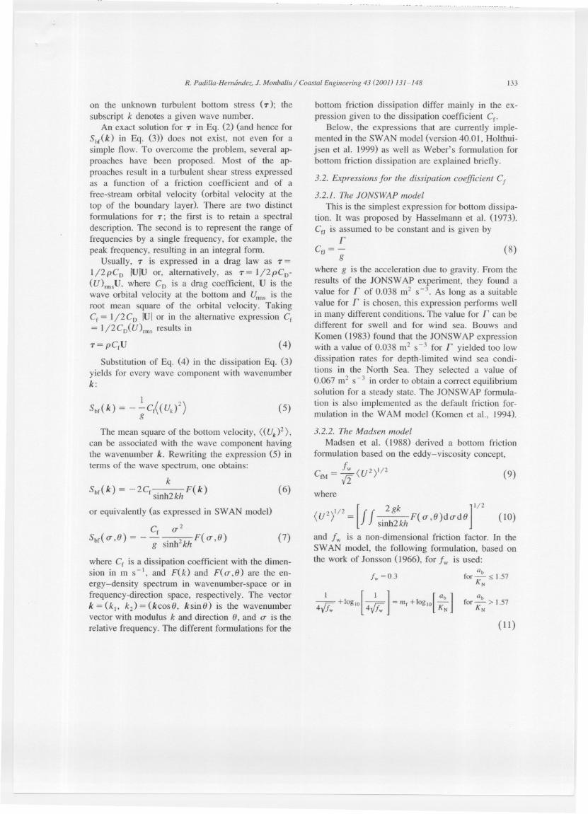
on the unknown turbulent bottom stress (T); thesubscript k denotes a given wave number.

An exact solution for T in Eq. (2) (and hence forSbf(k) in Eq. (3» does not exist, not even for asimple flow. To overcome the problem, several ap-proaches have been proposed. Most of the ap-proaches result in a turbulent shear stress expressedas a function of a friction coefficient and of afree-stream orbital velocity (orbital velocity at thetop of the boundary layer). There are two distinctformulations for T; the fIrst is to retain a spectraldescription. The second is to represent the range offrequencies by a single frequency, for example, thepeak frequency, resulting in an integral form.

Usually, T is expressed in a drag law as T =1/2pCD IUIU or, alternatively, as T= 1/2pCD-(U)rmsU, where CD is a drag coefficient, U is thewave orbital velocity at the bottom and Urmsis theroot mean square of the orbital velocity. TakingCf = 1/2CD IUIor in the alternativeexpressionCf= 1/2CD(U)rms results in

T=P~U (~

Substitution of Eq. (4) in the dissipation Eq. (3)yields for every wave component with wavenumberk:

Sbf(k) = - ~Cf(Uk/)g(5)

The mean square of the bottom velocity, «Uk)2 ),

can be associated with the wave component havingthe wavenumber k. Rewriting the expression (5) interms of the wave spectrum, one obtains:

kSbf(k) = -2Cf _._L'"u F( k) (6)

or equivalently (as expressed in SWAN model)

Cr a 2Sbf(a ,8) = - - . 2 F( a ,8)

g smh kh(7)

where Cr is a dissipation coefficient with the dimen-sion in m s- I, and F( k) and F( a , 8) are the en-ergy-density spectrum in wavenumber-space or infrequency-direction space, respectively. The vectork = (kl' k2) = (kcos8, ksin8) is the wavenumbervector with modulus k and direction 8, and a is therelative frequency. The different formulations for the

- -- - - -

133

bottom friction dissipation differ mainly in the ex-pression given to the dissipation coefficient Cf'

Below, the expressions that are currently imple-mented in the SWAN model (version 40.01, Holthui-jsen et al. 1999) as well as Weber's formulation forbottom friction dissipation are explained briefly.

3.2. Expressions for the dissipation coefficient Ct

3.2.1. The JONSWAP model

This is the simplest expression for bottom dissipa-tion. It was proposed by Hasselmann et al. (1973).CfJ is assumed to be constant and is given by

rCfJ = - (8)

g

where g is the acceleration due to gravity. From theresults of the JONSWAP experiment, they found avalue for r of 0.038 m2 S-3. As long as a suitablevalue for r is chosen, this expression performs wellin many different conditions. The value for r can bedifferent for swell and for wind sea. Bouws andKomen (1983) found that the JONSWAP expressionwith a value of 0.038 m2 S-3 for r yielded too lowdissipation rates for depth-limited wind sea condi-tions in the North Sea. They selected a value of0.067 m2 S-3 in order to obtain a correct equilibriumsolution for a steady state. The JONSWAP formula-tion is also implemented as the default friction for-mulation in the WAM model (Komen et aI., 1994).

3.2.2. The Madsen modelMadsen et al. (1988) derived a bottom friction

formulation based on the eddy-viscosity concept,

C = fw (U2 )1/2 (9)fM fi

where

[

2 k

]

1/2

(U2)1/2= ff . g F(a,8)dad8 (10)smh2kh

and fw is a non-dimensional friction factor. In theSWAN model, the following formulation, based onthe work of Jonsson (1966), for fw is used:

fw = 0.3

abfor- > 1.57

KN

(11)

----

134 R. Padilla-Hern/mdez. J. Monbaliu / Coastal Engineering 43 (200J) 131-148

where mr = -0.08, ab is a representative near-bot-tom excursion amplitude:

I

ab =[2ff . \ F( U ,O)dUdO

]2 (12)

smh kh

and KN is the bottom roughness length. Graber andMadsen (1988) implemented the expression of Mad-sen in a parametric wind sea model for finite waterdepths.

3.2.3. The Collins modelHasselmann and Collins (1968) derived a formu-

lation for the bottom friction dissipation. They re-lated the turbulent bottom stress to the external flowby means of a quadratic friction law. The dissipationcoefficient they derived reads:

Cr = 2C{ D;/U) + (U~)} (13)

where D;j is the Kronekerdeltafunction;( ) denotesthe ensemble average, U is equal to (U12+ Ul)I/2,U1 and U2 are the near bottom orbital velocitycomponents, and c is a drag coefficient determinedexperimentally as a function of the bottom rough-ness. Hasselmann and Collins proposed a value for cequal to 0.015.

Collins (I972) simplified the expression (13) forthe dissipation coefficient by leaving out the depen-dence on the direction of the wave component andby using the total wave induced bottom velocity:

Crc=2C(U2)2 (14)

where (U2) can be computed from Eq. (10). Ex-pression (14) is the one implemented in the SWANmodel. The value of the drag coefficient c was set to0.015. Cavaleri and Malanotte-Rizzoli (1981) imple-mented this friction model in a parametric wavemodel.

3.2.4. The Weber eddy-viscosity modelWeber's model for the spectral energy dissipation

due to friction in the turbulent wave boundary layeris based on the eddy-viscosity concept. In this model,the turbulent shear stress is parameterized in analogywith the viscous stress, with the coefficient of molec-ular viscosity replaced by a turbulent eddy-viscositycoefficient.

--

Solving the Navier-Stokes equations in the turbu-lent boundary layer and using perturbation theory,Weber derived the following dissipation coefficient.

(15)

CfW depends on the wave spectrum F(k), the waterdepth h, and the bottom roughness K N through thefriction velocity u', and on the radian frequency(w = 27TU) through ~o'

I I

=(

4( Yo+ h)w

)2 =

(

4KNw

)

2~0 . 30 '

KU KU(16)

The variable ~o reflects the ratio between theroughness length and the boundary layer thickness,which scales with u' / w; K is the von Kfumiinconstant set equal to 0.4; (Yo+ h) is the theoreticalbottom level and Tk is defined as

Tk is a dimensionless complex function and dependson the radian frequency and thus on the wavenumberthrough the argument ~o' Ker + iKei is the zeroorder Kelvin function (Abramowitz and Stegun,1965). The prime denotes the derivative with respectto the argument ~o' Details of the derivation of thedissipation coefficient in the eddy-viscosity modelare given in Weber (1989, 1991). It is of interest tolook at the differences and similarities between thedifferent formulations. The expression by Weber willbe used here as the reference since it models explic-itly the bottom friction dissipation mechanism.

The JONSWAP friction model does not interpretbottom dissipation in terms of a physical mechanismsuch as percolation, friction or bottom motion.

Weber's and Madsen's formulations differ in thefact that Madsen's model approximates the randomwave field by an "equivalent" monochromatic wave.This approximation is applied at an early stage oftheir calculations. Therefore, Madsen's expression isonly valid for a narrow, singled-peaked spectrum. Infact, Collins' drag-law dissipation expression is red-erived. However, in the Madsen formulation thefriction coefficient fw depends explicitly on the wavefield and on the roughness length.

---

R. Padilla-Hern(mdez, J. Monbaliu/ Coastal Engineering 43 (200/) /3/-/48

The formula of Weber is able to compute thedissipation rate directly from the bottom roughnesslength through the stress parameterization. That of-fers the possibility to adapt the dissipation rate ac-cording to the changing roughness under differentwave-current regimes. This could be important insome coastal areas. Moreover, the expression ofWeber maintains the spectral description and can beapplied to complex situations, where the wave fieldcannot be easily represented by one wave component(Weber, 1991).

4. Numerical experiments

4.1. 1ntroduction

In the following numerical experiments, the goalis to analyze the performance of the bottom frictionformulations of Hasselmann et a1.(1973), the eddy-viscosity model of Madsen et a1. (1988), the draglaw turbulent friction model of Collins (1972) andthe eddy-viscosity model of Weber (1989).

A comparison is made of SWAN model outputwith the data from the Lake George experiment(YV). The input files and the data for the SWANruns are taken from case F41LAKGR of the "Suite40.01.a of the bench mark tests for the shallow waterwave model SWAN Cycle 2, version 40.01(SBMSWAN)" (WL Delft Hydraulics, 1999).

4.2. Statistical analysis

In order to analyze the results from the SWANmodel using the different bottom friction models bycomparing them with measurements, a set of statisti-cal parameters following Dingemans (1997) is used:

The bias. The difference between the mean of theobservations (x) and the mean of the model results(y)

Bias = X - Y (18)

where Mean = X = ("i.jxJN), N is the number ofdata.

The rmse. The root mean square error

[

1 2

]

~

rmse = N ~ ( Yj - x;)(19)

135

The si. The scatter indexrmse

si = ill(20)

The re. The relative error or index of agreement

N X rmse2re=l-

pe

=1-

L (IYi -xl + IXj- XI)2i

(21 )

The relative error reflects the degree to which theobservations are approached by the model results.Willmott (1981) introduced re as an index of agree-ment. (re = 1, for perfect agreement, normally 0 < re< 1). The parameter pe is known as the potentialvariance.

In the computations of the different statisticalparameters, the imposed values of the wave parame-ters at the grid model boundary are not included inthe analysis.

4.3. Lake George

4.3.1. SituationThe Lake George experiment represents nearly

idealized wave growth in depth- and fetch-limitedconditions. The lake is fairly shallow with a relativeuniform bathymetry (depth about 2 m). It is approxi-mately 20 km long and 10 km wide. A series of eightwave gauges were situated along the North-Southaxis of the lake (Fig. 1).The bottom is rather smooth(bottom ripples were practically absent) and the bot-tom material consists of fine clay (Ris, 1997). Thewave measurements were carried out during the pe-riod from April 1992 until October 1993. Only datafor which the wind speed and direction were rela-tively constant during the 30-min sampling periodhave been retained. The criteria used for this selec-tion were that the wind speed should not vary bymore than 10% nor should the wind direction turn bymore than 10° to each side of the alignment of theinstrument array (north/south) during the 30-minsampling period. (For a complete description seeYV.)

--

136 R. Padilla-Hemandez. J. Monbaliu / Coastal Engineering 43 (200]) 131-148

Lake George Depth [m]o

" ~-O.5

<.

Fig. I. Bathymetry of Lake George and the locations of the eightwave gauges. Depth contour interval is 0.5 m starting from O.

For the computations, three northerly wind caseswere selected from the bench mark data set forSWAN (SBMSWAN, case F4ILAKGR). These casesare three typical examples, i.e., a low wind speed(UIO= 6.5 m S-I), medium wind speed (UIO= 10.8ms-I) and a high wind speed (UIO= 15.2 m s-t).

The computations were carried out with SWANversion 40.01 using the WAM Cycle 3 formulations(Booij et aI., 1999). The wave-wave triad interac-tions and depth-induced wave breaking were turnedon with default parameter values. For the bottomfriction, one of the above formulations is used. As inRis (1997), Station 1 is taken as the up-wave bound-ary in the simulation. This avoids uncertainty in thelocation of the northern shore because of seasonalvariation in water depth. Since no directional wavespectrum is available at Station 1, the directionaldistribution of the waves is approximated with acos2(1) directional distribution. For the computa-tions, a directional resolution of 10° and a logarith-mic frequency resolution (l1f= O.lf) between 0.166and 2.0 Hz for the low wind case and between 0.125and 1.0 Hz for the medium and high wind case arechosen. The spatial resolution is 250 m both in xand y direction. To account for seasonal variationsin water level, the water level was increased over theentire lake with +0.1, +0.3 and +0.27 m for thelow, medium and high wind case, respectively.

4.3.2. Calibration

In order to tune the friction coefficients of everyfriction model, the third case (high wind speed) waschosen. The combined scatter index (sic) for Hs andTp was taken as the cost function value to be mini-mized. The definition for the sic reads

sic = [si(Hs) + si(Tp)]/2 (22)

The results using the default value for the frictioncoefficient in every friction model is taken as areference (see Table I). An identical definition forthe combined relative error (rec) is used, replacing refor si in Eq. (22).

The si for Hs and Tp and the sic are shown in Fig.2. As can be observed in the figure, the behavior ofthe si is different for the different models. This

figure shows how sensitive the wave parameters (Hsand Tp) are to variations in the friction coefficient inthe case of the JONSWAP and the Collins expres-sions, and to variations in the roughness length, inthe case of the Madsen and the Weber expressions.

For the JONSWAP formulation and starting fromthe default value, it is clear that lowering the valueof the friction coefficient decreases the sic of Hs andTp. The si of Tp reaches a minimum at a value of0.030 m2 s-3 for r. For an interval of r-values, the

si of Tp is constant, but the results for Hs start

Table IFriction coefficient values for the different friction models and theresulting sicThe values in bold are the default and the underlined are the

optimal values for the Lake George case.

Run No. JONSWAP Madsen Collins Weber

r sic KN sic c sic KN sic[mm] [mm]

0.005 0.105 0.10 0.091 0.0005 0.120 0.01 0.0790.010 0.090 0.25 0.090 0.0025 0.106 0.10 0.0740.020 0.079 0.50 0.086 0.005 0.093 0.25 0.0710.025 0.074 1.0 0.080 0.010 0.089 0.50 0.0700.030 0.070 3.0 0.076 0.015 0.081 0.75 0.070-- - - --0.034 0.082 5.0 0.082 0.020 0.078 1.0 0.0740.038 0.080 10.0 0.093 0.025 0.074 2.5 0.1110.045 0.078 20.0 0.172 0.030 0.071 5.0 0.165--0.055 0.082 30.0 0.211 0.035 0.077 10.0 0.2030.067 0.092 50.0 0.214 0.040 0.081 20.0 0.2360.075 0.096 70.0 0.214 0.045 0.081 40.0 0.2410.085 0.120 80.0 0.214 0.060 0.085 60.0 0.242

I23456789

101112

R. Padilla-HemOndez. J. Monbaliu/ Coastal Engineering 43 (2001) 131-148

.2

u; .1r "'_"?"

j.....0.005 .020 .038 .067

r

.2

'r;; .1

1

.~'¥!!I...1

.0005 .005 .015c

137

'r;; .1~

~.....".-

......................

c;; .1

.0001 .0005 .05

WEBERr----

.2

",..,..~:....

...........-.....06 .0001 .00025 .01.04

KN

Fig. 2. The si for Hs and Tp. and sic in the function of the friction coefficient value in the Lake George case. The friction coefficient defaultvalue is indicated by a vertical line and the optimal value (the chosen value to run the three cases of Lake George) is indicated by a circle.

deteriorating. Nevertheless, lowering the value of rimproves the sic about 23% compared with theresults using the default value for r (see Table I).The value retained for r is 0.030. It should be noted

AP

.51 ~ I.3 TpCD .J.:

~ r-........1 j

0.005 .020 .038 .067r

CD'"E

.1, L /...............

o

.0005 .005 .015c

Fig. 3. Idem Fig. 2 but for rmse.

that the reference value for r was taken as 0.067,which is the appropriate value for depth-limitedwind-sea case in the Southern North Sea (Bouws andKomen, 1983), and not as 0.038 which corresponds

[EN

5 ..... .....3 ...

. ....CD .......en ..-E.......................

.1

.0001.0005 .005

KN

.05

.5

.3 ....................

..'.'.'.................

CD'"E

.1 o

.06 .0001 .00025 .01 .04

138 R. Padilla-Hern{mdez. J. Monbaliu / Coastal Engineering 43 (200]) 131-148

to swell conditions. The most suitable value for thiscase is even smaller than the value for swell condi-tions. The lowest value of the sic here cOITesponds

with the lowest value of si for Tp.Using the formulation of Madsen improvement of

sic leads to improvement for both Hs and Tp.That isbecause both parameters Hs and Tp are underesti-mated using the reference value. The optimal valuefor KN was chosen as 3 X 10-3 m. The improve-ment for the sic compared to the sic with the defaultvalue is about 64%. The lowest value of the sic doesnot cOITespondneither with the lowest value of the sifor Hs nor with the lowest value of the si for Tp.

The sic varies little using the formulation ofCollins for a region of c-values around the referencevalue. For higher than the reference value of c, the sifor Hs improves but the si for Tp increases. Going tolower values of c, the si of both wave parametersincreases. The value retained for c was taken equalto 0.030. According to Table 1 and Fig. 2, the sic hasthe best value but is only 14% different from the sicwith the default c-value. The value retained for c,however, does neither produce the lowest value ofthe si for Hs nor for Tp.Looking at the rmse (Fig. 3)and the rec (Fig. 4), it is not so clear that the wavemodel gives the best results for a c-value equal to0.030.

1.~N~~~:.............-::::: '

.8

2!

.6,,_ HsTp

--- rec0.005 .020 .038 .067

r

2!.6

For the friction model of Weber, lowering the sicleads to improvement for both Hs and Tp' Thechanges of the si are rather smooth making thechoice of the best value for KN easy. The optimalvalue for KN in Weber's formulation was chosenequal to 7.5 X 10-4 m. The improvement for the sicusing the optimum value compared to the sic withthe default value is about 71%.

Comparing the si, rmse and the re (Figs. 2, 3 and4, respectively), the results using the formulation ofWeber are more consistent in a statistical sense. Theoptimal value for KN' according to the sic costfunction, gives also the best value for the si, the rmseand the re for Hs' For Tp' the magnitude of thosestatistical parameters is quite close to the best values.That is not the case for the other formulations,especially not for the Collins' and Madsen's formu-lations. The lowest value for the sic (highest value ofrec) does not cOITespondneither to the lowest si andrmse (highest re) for Hs nor to the lowest si andrmse (highest re) for Tp. As can be seen in Figs. 2, 3and 4, the choice of the best value for the frictioncoefficient or the roughness length is prescribedmainly by the si of Tp. Tp is the parameter thatimproves most during the tuning process. Note thatRis et al. (1999) remarked that using the WAM cycle3 formulations, SWAN systematically overestimates

1.~~~.?~~ .'"----------.8

2!.6

.0001.0005 .005

KN

.05

.0005 .005 .015 .06 .0001 .00025 .01.04c KN

Fig. 4. Idem Fig. 2 but for there andrec.

R. Padilla-Hemimdez. J. Monba/iu I Coastal Engineering 43 (200]) 131-148

2f ·!468 0246

Stations Stations

Fig. 5. SW AN model results for the different bottom friction formulations (with the optimal value for the friction coefficients) and

observations of the significant wave height (left panels) and peak period (right panels) in nearly ideal generation conditions in Lake George.Observations (' ). JONSW AP ( + ). Madsen (v). Collins (0) and Weber (0) formulations.

the significant wave height and underestimates themean wave period.

It should be mentioned that a wave model run was

made using a roughness length corresponding to thegrain size at the bottom of the lake which is fine clay(Ris, 1997) of about I. X 10-6 m in diameter. Themodel was run using the expressions of Weber andMadsen. Comparing the results, using the expressionof Weber, between the retained value for KN (7.5 X10-4 m) and the roughness length corresponding tothe grain size (I. X 10-6 m) the sic increases byabout 30%. The si for Hs increases by 54% and thesi for Tp decreases by 12%. Using the Madsenexpression with KN equal to 1 X 10- 6 m, the differ-ence in the sic between the retained value for KN(3 X 10-3 m) and the roughness length correspond-ing to the grain size (1 X 10-6 m) is about 38%. Thesi gets worse by 13% for Tp and by 55% for Hs' Ascan be seen from these results, even at very smallvalues for KN the dissipation by bottom friction stillplays a role.

A wave model run without bottom friction for thecase of high wind speed was made to see howimportant the bottom friction is. The value of the sicnot considering the bottom friction is about 0.119.

Hs[m]

0.3 fU10=6.4 [m/s] . 0 0

0.21 .. t ~ ~ ~ ~.. .

0.1o 2 4 6

U10 =10.8 [n1Isl ...

0.4 f ~ i . ....

0.3L .t.-!

0.20 2 4 6

0.61U10 = 15.2 [m/S. ,..OAf ~.0.2

o 2

--

139

Comparing it with the value of 0.070, which isapproximately the value of the sic using the optimalcoefficients in the four bottom dissipation expres-sions (see Table 1), the difference is about 70%.

4.3.3. Validation

Once the appropriate values for the friction coeffi-cients and roughness length were chosen (see Table1, values underlined), the other two selected casesfor Lake George were run using these values. It isassumed that the bottom condition did not change.

As can be see in Fig. 5, the significant waveheight and the peak period are relatively well mod-eled by SWAN using either of the four frictionmodels, except at the last three stations in case one.At these stations (from 6 to 8), the wave parametersdo not show a monotonic behavior. That can possi-bly be ascribed to unresolved variation in the windfield. Such variation has been observed by YV.Those three stations were therefore eliminated from

the statistical calculations for case one only. A smallunderestimation of Tp can be observed in the mediumand low wind cases.

Fig. 6 shows the statistical parameters for thethree wind cases for each of the four bottom friction

B

2.22

1.81.6l ;1.4Le...

o 23

4 6 8

8

.$

$ $

6 84

2.5

8

---

2.5

21 ,:0 2.--------

3

140 R. Padilla-Hemcmdez, J. Monbaliu / Coastal Engineering 43 (200 J) J3J- /48

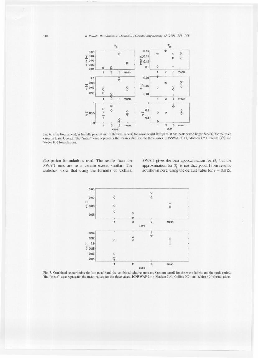
dissipation formulations used. The results from theSWAN runs are to a certain extent similar. The

statistics show that using the formula of Collins,

SWAN gives the best approximation for Hs but the

approximation for Tp is not that good. From results,not shown here, using the default value for c = 0.015,

0.08

0.07

~ 0.06

0.05

0.94

0.92

Z 0.9

~0.88

0.86

0.84

case

Fig. 7. Combined scatter index sic (top pane)) and the combined relative error rec (bottom pane)) for the wave height and the peak period.The "mean" case represents the mean values for the three cases. JONSW AP ( + ), Madsen ('\7), Collins (0) and Weber (0) formulations.

Hs Tp

0.05

0.161

ww '<7 8

I 0.04 0.14 0 00.03& 0.12

E 0.020.1 f 0 +

0.012 3 mean 1 2 3 mean

0.1

O5

0.08 - .."7""'0.06 0 60.06 8

0.04 0 0 0.042 3 mean 1 2 3 mean

0 8.:19

iO.95f0 0 .. g1 0.8

0.9' i2 3 mean 1 2 3 meancase case

Fig. 6. nnse (top panels), si (middle panels) and re (bottom panels) for wave height (teft panels) and peak period (right panels), for the threecases in Lake George. The "mean" case represents the mean value for the three cases. JONSWAP ( +), Madsen ('\7), Collins (0) andWeber (0) formulations.

'<7

Q+

':ijl

'<7

@0

0 0i

3 mean2case

+

000

0

¥ .3 mean

,2

R. Padilla-Hern(mdez. J. Monbaliu / Coastal Engineering 43 (200]) 131-148 141

Table 2

Fonnulas for non-dimensional energy (8) and non-dimensional frequency (11)against non-dimensional depth, obtained from the results ofSWAN using the different bottom friction models

Model JONSWAP Madsen Collins Weber

8=11=

4.1 X 10-381.76

0.148-0.472

2.9 X 10-38\.66

0.158-0.430

1.4 X 10-3 8\.42

0.208-0.375

1.4 X 10-3 8\.46

0.208- 0.375

T:r+j---0"H"T ;I>:r-+.:r.. -

~ --.,,--_--;1 :1

1

- YOUNG-- + JONSWAP

- - - MADSEN- COWNS

WEBER=10°

ere gives the worst approximation for Hs but thebest approximation for Tp.

Using the four bottom friction dissipation expres-sions, the largest error for Hs is in the high windcase compared with the other two cases. This can bepartially ascribed to a 'deviation' of the measure-ments from the monotonic behavior in the locations2 and 7 as can be seen in Fig. 5. Looking at themean values of rmse, si and re for the three cases(Fig. 6), the best performance for Hs corresponds tothe use of the Collins formulation and the best

performance for Tp corresponds to the Weber formu-lation. Fig. 7 shows the performance of the SWANusing the different bottom friction formulations inthe function of the combined statistics (sic and ree)

of Hs and Tp. As can be seen, SWAN has the bestperformance using Weber's formulation followed byCollins, and then by the JONSWAP and the Madsen

"'0

~10-4"b.

n'"

10-6

formulations. The peak period in the low wind case(for this wind field the bottom friction plays hardlyany role) is very well reproduced using the formula-tion of Weber. This is not the case using the otherformulations, as can be seen in Figs. 5 and 6.

4.3.4. Depth-limited wave growthIn order to refine the expressions of Bretschneider

(1958) for both non-dimensional energy (e) andnon-dimensional peak frequency (v), YV used theirfull data set of about 65,000 data points. They foundthat the asymptotic depth-limited growth can be con-sidered dependent on the non-dimensional depth (8)only. They found the following limits:

B = 1.06 X 10-3 81.3 (23)

v=0.208-o.375 (24)The non-dimensional parameters are defined as

g 2E / U1~ for the non-dimensional energy (B ),

Cl-0:)-0-n,.

/) - gdlu210

Fig. 8. Comparison of the SW AN results using the different bottom friction fonnulations and the fonnula from Young and Verhagen (1996)for non-dimensional energy 8 (top panel) and non-dimensional peak frequency 11(bottom panel) against non-dimensional depth.

142 R. Padilla-Hernfmdez. J. Monbaliu/ Coastal Engineering 43 (200]) /3/-/48

Table 3

Statistics comparing the values obtained from SWAN using thedifferent friction formulations with the values according to theformulae from YV in the case of depth-limited growth

Model JONSWAP Madsen Collins Weber

8 bias -0.002 -0.001 0.000 0.000rmse 0.003 0.002 0.000 0.000si 1.969 1.404 0.368 0.380re 0.800 0.816 0.955 0.953

v bias 0.055 0.055 0.000 0.000rmse 0.055 0.055 0.000 0.000si 0.243 0.241 0.000 0.000re 0.950 0.941 1.000 1.000

JpUIOIg for the non-dimensional peak frequency( v), gdI Ut~ for the non-dimensional depth (8), gis the gravitational acceleration, E is the total energyof the spectrum, UIOis the wind speed measured at areference height of 10 m, and d is the water depth.

To calculate the depth-limited growth, SWANwas run in one-dimensional mode for each of thefriction models. Several runs were performed usingdifferent depths ranging from 2.5 to 20 m. The windspeed was set equal to 20 m s-) (to work in thesame non-dimensional depth interval as YV). The

results were stored for different fetches ranging from15 to 15,000 km. The friction coefficients and rough-ness length used have the optimal values retainedfrom the tuning runs. The expressions given in Table2 were computed taking the maximum levels ofnon-dimensional energy and the minimum non-di-mensional peak frequency at every non-dimensionalfetch of the different runs.

Fig. 8 shows the different retained results for 8and v together with the expressions (23) and (24) ofYV. Table 3 shows the statistics comparing themwith the formulas obtained by YV. Although all ofthem give a good approximation to the measure-ments, it is clear that the formulae of Weber andCollins give the best results. The fit to the v curve ofYV is perfect. Because of the good approximation ofall formulations to the formula from YV, Table 3confirms that selecting sic as the parameter to beminimized was a good selection.

Even though YV considered that the asymptoticdepth-limited energy growth depends on non-dimen-sional depth only, the numerical results show that thedepth-limited growth is a function of the roughnesslength as well. If the bottom friction and bed mate-rial were not important in fetch- and depth-limited

10-6

- YOUNG+ Kn.10

- - Kn.025. Kn.0025- - - Kn.OOO25- Kn.00005

10°

/) =gdIu210

Fig. 9. Comparison of the SW AN results using the formulation of Weber with different roughness length (KN) and the formula from Young

and Verhagen (1996) for non-dimensional energy 8 (top panel) and non-dimensional peak frequency v (bottom panel) against non-dimen-sional depth.

- --

R. Padilla-Hemandez. J. Monbaliu / Coastal Engineering 43 (2oon /3/-/48

conditions (as assumed by YV), then the value as-signed to KN should not matter and the resultswould be expected to be the same. This is not thecase when the wave model is run using a differentroughness length in the friction dissipation formula-tion. To exemplify this, the SWAN model was runfor depth-limited wave growth with Weber's formu-lation for bottom friction. Fig. 9 shows the results fordifferent values for K N' Going from larger to smallervalues of KN' the e increases and the v decreases.Hence, one should expect that the curves for egrowth against non-dimensional fetch change as well.This implies that the expressions (23) and (24) shouldtake into account the bottom roughness. The asymp-totes for e and v can be expressed as:

(25)

(26)

One can see from Fig. 9 that the roughness lengthhas more influence on A and C than on Band D.

Changing KN from 0.10 to 5 X 10-5 m, A changesaround 250%, B changes 8%. C and D change 30%and 9%, respectively. KN has more impact on theenergy than on the frequency. This suggests that Aand C are functions of K N.

4.3.5. Fetch-limited wave growthUsing their data from Lake George, YV proposed

a generalized form to the shallow water limits for thegrowth of non-dimensional energy (e) and non-di-mensional peak frequency (v) with non-dimensionalfetch ( X)

e=3.64XIO-3{

tanhA\tanh [ BI

]}n (27)tanh A \

V=0.133{tanhA2tanh

[

B2

]}m (28)

tanh A2

where

(29)

(30)

143

and X is the non-dimensional fetch. (X = gx/ U1~),x is the distance and

A2 = 1.5051/m B-O.375/m

B2 = 16.3911/m X-O.27/m

(31 )

(32)

The coefficients n and m control the rate oftransition from "deep" to "depth limited" conditions.YV performed a non-linear least squares analysis ontheir selected data set to determine nand m. Theiranalysis yielded n equal to 1.74 and m equal to-0.37. Expressions (27) and (28) give a family ofcurves, one for each value of B.

The results from SWAN are compared with theequations given by YV. Figs. 10 and 11 show theresults from SWAN using the different bottom fric-tion formulations for B equal to 0.10 and 0.50,respectively. The deep water asymptotic forms ofEqs. (27) and (28) and the same equations but forshallow water (n equal to 1.74 and m equal to- 0.37) are also shown. As can be seen from thosefigures, SWAN overestimates the total energy forvery short X. In particular, energy growth in thehigh frequency range (very short fetches) is usuallyoverestimated by SWAN. This overestimation is ob-served systematically. According to Ris et al. (1999),the overestimation of energy at short fetches can beascribed to the linear wave growth term of Cavaleriand Malanotte-Rizzoli (1981). But in this work, thelinear growth term was not taken into account. Re-sults from the wave model using the linear wavegrowth shows no relevant differences with the resultswithout the linear growth term. The observed overes-timation of energy should be ascribed to anotherreason. The search for such reason is beyond thescope of this work.

The SWAN runs with the formulations of Collinsand Weber for bottom friction dissipation catch theasymptotic levels of e and v given by the expres-sion of YV quite well, better than when using theexpressions of JONSWAP and Madsen. But as canbe seen in Fig. 11, the wave model reproduces betterthe levels of non-dimensional energy when using theexpression of Weber than when using the expressionof Collins.

To quantify the differences between the modelresults and the expression of YV for fetch-limitedgrowth, the wave model was run for a range of

144 R. Padilla-Hem(mdez. J. Monbaliu/ Coastal Engineering 43 (200]) 131-148

.. o;:i"

~ 10"11'"

"""'-'-------

10.11~ 1~

X.=gx/l.r\oFig. 10. (a) Non-dimensional energy ISand (b) non-dimensional peak frequency 11against non-dimensional fetch X for a non-dimensionaldepth {j of 0.10. The deep water asymptotic form of Eqs. (20) and (23) is shown in dashed line. The same equations but for shallow wateras found by YV (n = 1.74 and m = - 0.375) is in solid line. SWAN was run using JONSW AP ( +), Madsen (v), Collins (0) and Weber( 0) formulation.

values of B. The four statistical parameters given inSection 4.2 are computed.

Fig. 12 shows the statistical parameters compar-ing I> from the wave model results against the I>

------------

103

X.= gx/lF,o

Fig. 11. Idem Fig. 10 but for a non-dimensional depth {j of 0.50. SWAN was run using JONSW AP ( + ), Madsen (0), Collins (dotted) andWebers (0) formulations.

--- ---- --

10.3

.. 0;:i"

10"

n'" 0

10.5102

100 b

103

<» I

0

-0n

;:i"_0-I>

R. Padilla-Hemlmdez. J. Monba/iu / Coastal Engineering 43 (200J) 131-148

X 10-41

a

o

-1gjJ5 -2

-3

-40

~"' ft::---"'"... "~ '"

........-.............

8

0.5

C

0.5/i

145

Eb

3

..

~21

1

..........-........r----

"vr., ,..-.....oo 0.5

d

0.5/i

Fig. 12. The bias. nnse, si and re against non-dimensional depth 8. The comparison is done for wave growth in fetch-limited conditionsbetween the non-dimensional energy & from SW AN with the different bottom friction dissipation fonnulations and the fonnula from Young

and Verhagen (1996).

computed from the YV expression (Eq. (27» for arange of values of 8. Fig. 13 shows the same as Fig.12 but for v. In this way, Figs. 10 and 11 arerepresented statistically in Figs. 12 and 13 as two

points at 8-values of 0.10 and 0.50, respectively. Tocalculate the fetch-limited growth, SWAN was run inone-dimensional mode for each of the friction mod-

els. Several runs were performed using a depth equal

""'-, '\'\I '..J; ".., ......

~ .~ 0.70.5 1 0 0.58 /i

Fig. 13. Idem Fig. 12 but for non-dimensional frequency.

0.5

oo

d

0.9

I!!0.8

0.06, av

, -.ION ' 0.5

o.04f '- 0.4...... COL

o.o:t

'-_, --- WEB .. 0.3"'

"" ,"-"S 0.2

, .... ..../\ ........ '. 0.1.. ""',, ...

-0.02' \' ,..-.........0 0.5

1.5 C

146 R. Padilla-Herncmdez. J. Monbaliu / Coastal Engineering 43 (200J) 131 - 148

to 20 m and wind speedrangingfrom 10 to 31.3 ms-1 (to work in the non-dimensional depth rangefrom 0.1 to 1.0). The total fetch for every run was15,000 km with a resolution of 5 km. The fetch tocompute the statistical parameters was different forevery 8, depending on when the energy computedfrom Eq. (27) becomes constant (no changes in theseventh significant digit). The fetch range is from440 km for 8 equal to 0.1 to 997 km when 0 isequal to 1.0. At small D-values,SWAN gives resultswhich have almost the same bias and rmse usingeither of the four bottom friction dissipation expres-sions. From Fig. 12a and b, it is evident that resultsstart diverging going to deeper waters. At higherD-values, the use of the expressions of JONSWAPand Madsen gives the largest bias and rmse. Apply-ing the formulations of Collins and Weber, oneobtains smaller bias and rmse, with a preference forWeber's expression. Looking at the four statisticalparameters (Fig. 12), the results of SWAN using theformula of Weber approach better the non-dimen-sional energy 8 computed by Eq. (27) and its behav-ior is more uniform along the non-dimensional depthaxis, as can be seen in Fig. 12d.

Fig. 13 shows the statistics for the non-dimen-sional frequency v of the SWAN results using thedifferent bottom friction dissipation formulations. Incontrast with 8, the bias and the rmse of v do nothave the same value for small o. Contrary to theresults for 8, the bias and the rmse decrease withincreasing 8.

The statistical measures for 8 indicate that usingthe expressions of Weber the wave model resultsapproach quite well the values computed from Eq.(27), better than using the other three bottom frictionformulations. With respect to v, the wave results areof similar quality when the expressions of Collinsand Weber are used and better than when using oneof the other two expressions.

One can therefore conclude that in fetch- anddepth-limited conditions, the computed wave param-eters are more consistent when the bottom frictiondissipation expression of Weber is used.

5. Summary and conclusions

The main objective was to investigate and clarifywhich bottom friction formulation performs best or

is more consistent in shallow water regions. TheSWAN model was run with the three formulationsoriginally included plus the eddy-viscosity formula-tion of Weber. The data of Lake George were usedto tune the friction coefficients of every formulationsuch that the combined scatter index was minimal.This exercise revealed different levels of difficulty intuning the different friction coefficients.

Weber's model showed the best performance inthe cases of depth- and fetch-limited wave growth. Inthe case of depth-limited wave growth, the fit of thecalculated curve for the non-dimensional peak fre-quency to the one obtained by YV is as good asperfect. For the non-dimensional energy, the statisti-cal values, rmse, si and re, show that the resultsusing Weber's formulation are superior in approach-ing the equations obtained from YV. In the case offetch-limited wave growth, the formulation of Webershowed the best performance in approaching theequations of YV derived from the measurements.Running the SWAN model using Weber's formulawith different roughness length suggests that in theequations for depth- and fetch-limited wave growththe effect of bottom roughness should be included.

Formulations for dissipation by bottom friction,such as the model by Madsen or Weber, which takeexplicitly physical parameters for bottom roughnessinto account, should be preferred in wave modelingin shallow water areas. They offer the possibility toadapt the dissipation rate according to the changingroughness under different wave or wave-currentconditions.

Besides showing the best performance, the for-mula of Weber has some other advantages. It was, atleast for the Lake George case, easier to tune thanthe other formulations. The tuning parameter, namely,the bottom roughness length has a physical meaning.It gives information about the bottom boundary layer,through the friction velocity. It retains a spectraldescription making this formulation more reliable fora multi-modal wave spectra. It can be extended tothe combined wave-current situation, important insituations where the tidal currents play a significantrole in the dynamics of the coastal zone.

The above conclusions are based on two majorassumptions. The first assumption states that thebottom friction dissipation is the only 'unknown'source term and the other source terms are repre-

147R. Padilla-Hemfmdez. J. Monba/iu / Coastal Engineering 43 (200J) 131-148

sented cOlTectly. The second assumption states thatthe conclusions would be the same if the bottomcharacteristics of the Lake George would, for exam-ple, change from fine clay to a sandy bottom. Itwould therefore be interesting to redo the aboveexercise when better formulations for the other sourceterms and/or when similar measurements but in asituation with a different bottom material becomeavailable.

Notation

ab Near bottom excursion-amplitude [m]C Coefficient in the Collins expression for the

dissipation coefficient [-]Non-dimensional friction factor [-]Dissipation coefficient [ms-I ]JONSWAP dissipation coefficient [m s-I]Madsen dissipation coefficient [m s- I]Collins dissipation coefficient [m s- I]Weber dissipation coefficient [m s-I ]

Cx' Cy Wave propagation velocities in geographi-cal X-, y-space [m s-I]

ccr' Co Wave propagation velocities in spectral eT-,O-space[S-2, rad s- I]Water depth [m]Total energy of the wave spectrum [m2]Frequency [Hz]Energy density spectrum [m2 s rad- I]Acceleration due to gravity [m S-2]Total water depth [m]Significant wave height [m]Wavenumbervector[m- 1]Wavenumber [m-I]Roughness length [m]Wave action density [m2 S2 rad-1]Reynolds-average pressure [N m- 2]Relative elTor [-]Combined relative elTor = (re( H.) + re-(Tp))/2 [-]Root mean square elTor[-]Dissipation of wave energy by bottom fric-tion [m2 s rad-I]Dissipation due to depth-induced wavebreaking [m2 s rad- I]Dissipation by wave friction [m2 s rad-I]Non-linear wave-wave interactions [m2 srad- I]Scatter index [-]

dE

fF

gh

Hskk

KNN

prerec

si

Combined scatter index = (si(Hs) + si-

(Tp))/2 [-]Time [s]Wave peak period [s]Reynolds-average velocity [m s- I]Friction velocity at the bottom [m s-I ]Orbital velocity at the bottom for a givenwave number [m s-I ]Wind speed at 10 meters above the waterlevel [m S-I]

<u 2>1/2 Root meansquareof the orbitalmotionatthe bottom [m s- 1]Horizontal coordinates [m]Vertical coordinate [m]Coefficient in CfJ [m2 s- 3]Non-dimensional depth [-]Kronecker delta [-]Non-dimensional energy [-]Wave direction [rad]von Karman constant [-]Non-dimensional peak frequency [-]Density of the water [kg m- 3]Relative frequency [rad]Turbulent stress in the wave boundary layer[N m -2]Non-dimensional fetch [-]Radian frequency [rad s- 1]

sic

.u

x, y

oK

v

peT'T

xw

Acknowledgements

R.P.H. gratefully acknowledges financial supportfrom the Consejo Nacional de Ciencia y Tecnologla(CONACYT,Mexico). We also thank WL DelftHydraulics for the SBMSWAN and Ian Young, Uni-versity of New South Wales, CanbelTa,Australia, forthe data of Lake George.

References

Abramowitz, M.. Slegun, LA., 1965. Handbook of Mathematical

Functions. National Bureau of Standards, Washington, DC.

Booij, N., Ris, R.c., Holthuijsen, L.H., 1999. A third-generationwave model for coastal region: 1. Model description and

validation. J. Oeophys. Res. 104 (C4), 7649-7666.Bouws, E., Komen, 0.1., 1983. On the balance between growth

148 R. PadiLla-Hern[mdez. J. Monbaliu / Coastal Engineering 43 (200]) 131-148

and dissipation in an extreme, depth limited wind-sea in theSouthern North Sea. J. Phys. Oceanogr. 13, 1653-1658.

Bretschneider, e.L., 1958. Revised wave forecasting relationships.Proc. 6th Conference on Coastal Engineering, Gainesville/

Palm Beach/Miami Beach, FL. ASCE, New York, pp. 30-67.Cavaleri, L., Malanotte-Rizzoli, P., 1981. Wind wave prediction

in shallow water: theory and application. J. Geophys. Res.86-CII, 10961-10973.

Collins, J .1., 1972. Prediction of shallow water spectra. J. Geo-

phys. Res. 93 (Cl), 491-508.

Dingemans, M.W., 1997. Water Wave Propagation Over UnevenBottoms: Part I. Linear wave propagation. Advanced Series

on Ocean Engineering, vol. 13, World Scientific, Singapore.Graber, Re., Madsen, O.S., 1988. A finite-depth wind wave

model: 1. Model description. J. Phys. Oceanogr. 18, 1465-1483.

Hasselmann, K., Collins, J.I., 1968. Spectral dissipation of finite-

depth gravity waves due to turbulent bottom friction. J. Mar.Res. 26 (I), 1-12.

Hasselmann, K., Bamett, T.P., Bouws, E., Carlson, H., Cartwright,

D.E., Enke, K., Ewing, J.A., Gienapp, H., Hasselmann, D.E.,Kruseman, P., Meerbrug, A., Mliller, P., Olbers, DJ., Richter,K., Sell, W., Walden, H., 1973. Measurements of wind-wave

growth and swell decay during the Joint North Sea WaveProject (JONSWAP). Dtsch. Hydrogr. Z., A 80 (12),95 pp.

Holthuijsen, L.H., Booij, N., Ris, R.e., Haagsma, Ij.G., Kieften-

burg, A.T.M.M., Padilla-Hernandez, R., 1999. SWAN Cycle 2version 40.01. User Manual. Delft University of Technology,The Netherlands.

Jonsson, I.G., 1966. Wave boundary layers and friction factors.

Proc. 10th Int. Conf. Coastal Engineering. ASCE, Tokyo,

Japan, pp. 127-148.Komen, GJ., Cavaleri, L., Donelan, M., Hasselmann, K., Hassel-

mann, S., Janssen, P.A.E.M., 1994. Dynamics and Modelling

of Ocean Waves. Cambridge Univ. Press, Cambridge, 532 pp.

Luo, W., Monbaliu, J., 1994. Effects of the bottom friction

formulation on the energy balance for gravity waves in shal-

low water. J. Geophys. Res. 99 (C9), 18501-18511.Madsen, O.S., Poon, Y.-K., Graber, H.C., 1988. Spectral wave

attenuation by bottom friction: theory. Proc. 21 st Int. Conf. on

Coastal Eng. ASCE, Malaga, Spain, pp. 492-504.Putrnan, J.A., Johnson, J.W., 1949. The dissipation of wave

energy by bottom friction. Trans. Am. Geophys. Union 30,67-74.

Ris, R.e., 1997. Spectral modelling of wind waves in coastal

areas. PhD thesis. Delft University of Technology, TheNetherlands.

Ris, R.e., Holthuijsen, L.H., Booij, N., 1999. A third-generation

wave model for coastal region: 2. Verification. J. Geophys.Res. 104 (C4), 7667-7681.

Shemdin, P., Hasselmann, K., Hsiao, S.V., Herterich, K., 1978.Non-linear and linear bottom interaction effects in shallow

water. Turbulent Fluxes Through the Sea Surface, Wave Dy-namics and Prediction. NATO Conf. Ser. V, vol. I, pp.347-372.

Weber, S.L., 1989. Surface gravity waves and turbulent bottom

friction. PhD thesis. University of Utrecht, the Netherlands.Weber, N., 1991. Bottom friction for wind sea and swell in

extreme depth-limited situations. J. Phys. Oceanogr. 21 (I),149-172.

Willmott, CJ., 1981. On the validation of models. Phys. Geogr. 2(2), 219-232.

WL Delft Hydraulics, 1999. SBMSWAN (Suite 40.01.a of theBenchmark Test for the Shallow Water Wave Model SWAN

Cycle 2, version 40.00. Edited by Delft University of Tech-nology.

Young, I.R., Verhagen, L.A., 1996. The growth of fetch limited

waves in water of finite depth: Part 1. Total energy and peak

frequency. Coastal Eng. 29,47-78.

---