Endogenous Uncertainty and Rational Belief Equilibrium: A Unified Theory of Market Volatility

by

Mordecai Kurz

Stanford University, July 14 1999Presented at the International School of Economic Research in Siena July 5 - 11, 1999

Department of EconomicsSerra Street at GalvezStanford UniversityStanford, CA. 94305-6072e-mail: mordecai@leland.stanford.eduhttp://www.stanford.edu/~mordecai

Abstract. The theory of Rational Belief Equilibria (RBE) offers a unified paradigm for explaining market volatility bythe effect of "Endogenous Uncertainty" on financial markets. This uncertainty is propagated within the economy (hence"endogenous") by the beliefs of asset traders. The theory of RBE was developed in a sequence of papers assembled in arecently published book (Kurz [1997]) and the present paper provides an exposition of both the main ideas of the theoryof RBE as well as a summary of the main results of the book regarding market volatility.

Section I starts by reviewing the standard assumptions underlying models of Rational Expectations Equilibria(REE) and their implications to market volatility. The paper then reviews four basic problems which have constitutedpuzzles or anomalies in relation to the assumptions of REE : (i) Why are asset prices much more volatile than theirunderlying fundamentals? (ii) The equity premium puzzle: why under REE is the predicted riskless rate so high and theequity risk premium so low? (iii) Why do asset prices and returns exhibit the "GARCH" behavior without exogenousfundamental variables to explain it? (iv) The "Forward Discount Bias" in foreign exchange: why are interest ratedifferentials poor predictors of future changes in the exchange rates? Section II outlines the basic assumptions of thetheory of RBE and the main propositions which it implies for market volatility. Section III develops the simulationmodels which are used to study the four problems above and explains that the domestic economy is calibrated, as inMehra and Prescott [1985], to the U.S. economy. Then for each of the four problems the relevant simulation results ofthe RBE are presented and compared to the results predicted by a corresponding REE and to the actual empiricalobservations in the U.S.

The paper concludes that the main cause of market volatility is the dynamics of beliefs of agents. The theory ofRBE shows that if agents disagree then the state of belief of each agent, represented by his conditional probability, mustfluctuate over time. Hence the distribution of the individual states of belief in the market is the root cause of allphenomena of market volatility. The GARCH phenomenon of time varying variance of asset prices is explained in thesimulation model by the presence of both persistence in the states of beliefs of agents as well as correlation among thesestates. Correlation makes beliefs either narrowly distributed (i.e. "consensus") or widely distributed (i.e. "non-consensus"). In a belief regime of consensus (due to persistence it remains in place for a while) agents seek to buy orsell the same portfolio leading to high volatility. In a belief regime of non-consensus there is a widespread disagreementwhich causes a balance between sellers and buyers leading to low market volatility. In short, the GARCH phenomenonis the result of shifts in the distribution of beliefs in the market induced by the dynamics of the individual states of belief.

Turning to the equity risk premium, the key question is what are the distributions of beliefs which ensure thatthe average riskless rate is low and the average equity risk premium is high. It turns out that the only circumstanceswhen the mean riskless rate falls to around 1% and the mean equity premium rises to around 7% arise when, on theaverage, the majority of agents are relatively optimistic about the prospects of capital gains in the subsequent period. Insuch a circumstance the rationality of belief conditions imply that the pessimists (who are in the minority) must have ahigher intensity of pessimism than the intensity of the optimists. In a large economy with this property the state of beliefof any one agent may fluctuate but on the average there will be a minority of intensely pessimistic agents. Thisasymmetry between optimists and pessimists flows directly from the rationality conditions of beliefs and implies that atmost dates the pessimists have a stronger impact on the bill market. At those dates the pessimists protect their wealth byincreasing their purchases of the riskless bill. This bids up the price of the bill, lowers the riskless rate and results in ahigher equity risk premium. In sum, the theory of RBE offers a very simple explanation to the observed riskless rate andequity premium. It says that the riskless rate is, on average, low and the premium high because at most dates there is aminority of pessimist who, by the rationality of belief conditions, have the higher intensity level of belief about highstock prices in the future. These agents drive the riskless rate lower and the equity premium higher.

The "Forward Discount Bias" in foreign exchange markets is the result of the fact that in an RBE agents oftenmake the wrong forecasts although they are right on the average. Hence, in an RBE the exchange rate fluctuatesexcessively due to the errors of the agents and hence at almost no date is the interest differential between two countriesan unbiased estimate of the rate of depreciation of the exchange rate one period later. The bias is positive since agentswho invest in foreign currency demand a risk premium on endogenous uncertainty which is above and beyond the riskwhich exists in an REE. The size of the bias is equal to the added risk premium due to endogenous uncertainty.

JEL Classification Numbers: D58, D84, G12.Key Words: rational expectation equilibrium (REE), rational beliefs, rational belief equilibrium

(RBE), endogenous uncertainty, state of belief, market volatility, equity risk premium,riskless rate, GARCH, forward discount bias, foreign exchange rates, OLG economy,correlation among beliefs, simulations.

This work has been supported by Fondazione ENI Enrico Mattei, Milano, Italy. I thank Horace W.1

Brock, William A. Brock, Michael Magill and Martine Quinzii for extremely valuable comments on an earlierdraft of this paper. I thank Stanley Black and Maurizio Motolese for their dedicated assistance.

1

Endogenous Uncertainty and Rational Belief Equilibrium: A Unified View of Market Volatilit y

by

Mordecai Kurz1

I. The Basic Issue

This paper surveys the unified view of market volatility that flows from the insight thatvolatility has two components. One is generated by "fundamental" forces which are outside theeconomy and I refer to them as exogenous. The second is propagated within the economicsystem and I refer to it as the endogenous component. Since the nature of exogenous shocks iswell known, explaining the endogenous component is the main task of this paper. My expositionstyle in this survey is mostly non-technical but several sections are mathematically formal in orderto ensure that a precise statement of the main concepts is provided.

Before explaining my theory, I briefly outline the perspective of the Market EfficiencyTheory, or Rational Expectations Equilibrium (REE) on market volatility. My aim is to use REEas a reference point for the evaluation of the problems which market volatility generates. Myaccount is brief since the theory of REE is well known.

The standard formulation of an equilibrium of an economy starts with the dynamicportfolio and consumption choices of households and the production, investment and dividenddecisions of firms. The theory is closed with market clearing conditions but given the randomnature of the underlying economy it follows that equilibrium quantities are all stochastic processeswith an underlying probability law. I call this probability the "true" probability law. Most of whatis done in modern research depends upon the utilization of this probability for computing objectslike forecasts, theoretical covariances or security prices. Thus, the idea that equilibrium isrepresented by a true stochastic process is fundamental to modern thinking in economics.

The REE theory is based on several assumptions, but three of them are fundamental to mydiscussion here. These are:

(A.1) The true probability law of the economy is stationary. In a stationary economy thejoint probabilities of economic variables remain the same over time.

(A.2) Economic agents know the true probability law underlying the equilibrium variablesof the economy. This is the first component of "structural knowledge" which the agents

2

are assumed to possess.(A.3) Agents know the demand and supply functions of all other agents. They cancompute equilibrium prices of commodities and assets in the present and in the futuregiven any possible exogenous fundamental information in the future. This is the secondcomponent of structural knowledge which they possess.

When formulating uncertainty, the standard theory specifies an exogenous "state space"which describes all that the agents are uncertain about with respect to the external environment. Examples of exogenous variables include: weather conditions, earthquakes, technologicalchanges, fire destruction etc. All equilibrium magnitudes depend upon the realization of theexogenous state but according to (A.3) all agents know the map between equilibrium magnitudes(e.g. production decisions of firms, prices, etc.) and the state. Consequently, all economicmagnitudes vary only with the variability of the exogenous state over time. Moreover, it is thenan assumption that given any observed information, all agents agree on the interpretation of suchinformation.

The implication of these assumptions is that all financial risks and observed volatility arisefrom causes which are external to the economy. I call such uncertainty "ExogenousUncertainty". Under the above theory, no risk can be propagated from within the economicsystem via human beliefs or actions and the volatility of equilibrium variables is exactly equal tothe level justified by the variability of exogenous conditions.

The above discussion enables me to offer a simple summary of the conclusions of thetheory of REE with respect to the nature of market volatility:

1. For each state of the exogenous fundamentals there is a correct equilibrium price of allsecurities in the market.2. If you possess all exogenous fundamental information you are able to compute thecorrect prices of securities and hence all uncertainty about prices is resolved. Byimplication, hedging against the risks of all exogenous fundamentals is possible, inprinciple, and can control all risk associated with market volatility.3. All market volatility is caused by exogenous forces.

These conclusions of REE have been at the foundation of contemporary research into thestructure of market volatility. Unfortunately, they are in conflict with many empiricalobservations and with common experience of market participants. Indeed, the implications ofthis theory have been rejected in broad areas of economics. In order to discuss specific issues Inote that there are several outstanding problems or paradoxes (sometimes called "anomalies")related to the functioning of financial markets which the REE theory failed to resolve and currentacademic research has aimed to develop special theories to explain each one of these paradoxes. Since I will offer a unified view of market volatility, such a single theory would be moreconvincing if it could solve simultaneously many of these problems. Here I focus on four centralsuch problems:

Models of "Noisy" rational expectation equilibria have also attempted to address this problem2

within the rational expectations paradigm. In these models the noise in prices is assumed to be generated bythe erratic trades of "noise traders" who are uninformed and irrational traders constituting a significantproportion of all traders in the market. I do not review this work in the present paper since it stands in sharpcontrast to the basic rationality postulates of that paradigm. That is, since all the conclusions of a model ofnoisy rational expectations are driven by the arbitrary market actions of irrational traders, such a modelshould be viewed as a theory of irrational behavior with which one can prove anything. Also, from theempirical perspective it is hard to see who these noise traders are and since on average they lose money it isnot clear what makes such traders survive.

Kurz (ed) [1997] Endogenous Economic Fluctuations: Studies in the Theory of Rational Beliefs.3

Studies in Economic Theory No. 6, Berlin and New York: Springer-Verlag. The introductory Chapter 1(Kurz [1997a]) and the "Applications" Part B consisting of Chapters 9, 10, 11 and 12 contain the detailswhich explain the ideas and support the results reported in the present paper.

3

& Problem A: Why are asset prices and foreign exchange rates much more volatile thantheir underlying fundamentals?& Problem B: Why do models based on REE predict an equity risk premium over theriskless rate of around .5% and a rate of return on riskless short term debt of around 5.5%while over the last hundred years the average equity risk premium in the U.S. has beenaround 7% and the riskless rate has been around 1%?& Problem C: Why do asset prices and returns exhibit the "GARCH" behavior of timevarying variances when there are no fundamental factors to explain it?& Problem D: Why have interest rate differentials (between two countries ) been suchpoor predictors of future changes in foreign exchange differentials in contrast with rationalexpectations, giving rise to the "Forward Discount Bias"?

Those who rejected the theory of rational expectations have tended to drift in diversedirections. Some have concluded that financial markets are dominated by investors who perceiveprobabilities incorrectly or are vulnerable to the impact of fads and mass psychology. Othershave concluded that for some unexplained reason the market can be irrational sometimes and eachfailed prediction of the theory has been ascribed to a corresponding incident of such irrationality. As a result, it is common to find in the investment community the argument that each instant ofsuch presumed irrationality offers an opportunity for excess returns (i.e. when an investmentopportunity is viewed as "excellent" and inexpensive). These perspectives are in conflict bothwith principles of rationality as well as with the hope of finding one explanation for all thesephenomena. This is my motivation for seeking a unified theory for market volatility.2

I proceed by reviewing in Section II the basic premises of my theory of Rational Beliefsand the allied concept of "Endogenous Uncertainty" which are the cornerstones of my approach. Section III, which is the main section of this paper, is devoted to showing via simulation resultshow the theory which I propose resolves the four Problems outlined. Most of the materialpresented here is based on papers published in a volume by Kurz (ed)[1997] and on Kurz and3

Motolese [1999].

xt � X I ÜN

(X)� (X)�

(X)� (X)� (X)�

(X)� (X)�

(X)� (X)�

(X)� TnB Tn

4

II. Endogenous Uncertainty and Rational Beliefs

II(A) Rational BeliefsMy theory of Rational Belief Equilibrium (RBE) developed in Kurz [1994a], [1994b] is

based on the following alternative assumptions:

(AA.1) Despite the fact that the economy may undergo structural changes yielding non-stationarity, the economic universe is stable in the sense that statistical and quantitativeanalysis can be successfully carried out in it. In such a system the concept of "normal"patterns makes empirical sense and provides useful knowledge. It is represented by thelong-term averages of economic variables. Thus, although our economy experiencestechnological and economic changes, the price/earning ratios of major indices have wellknown "normal" ranges and long-term (i.e. asymptotic) means, variances and covariances. Interest rates, growth rates, capital/output ratios etc. all have well known long-runaverage behavior which reveals some important dimensions of the true structure of theeconomy.

(AA.2) Economic agents do not know the true probability law underlying equilibriummagnitudes. This is the first component of structural knowledge which agents areassumed to lack.

(AA.3) Agents do not know the map from exogenous variables to equilibrium quantities ingeneral and prices in particular. They have, however, access to the very large volume of allpast data on the performance of the economy. This data they can use to statistically testany theory which they may develop about the functioning of the economy and of thefinancial markets. In this sense agents may learn something about structural relationshipsin the economy.

In formal terms, let be a vector of all observables at date t and assume it tobe N, finite. The sequence {x , t = 0, 1 ,...} is a stochastic process with true probability $. I uset

the notation x = (x , x , . . .) for members of and denote by %( ) the Borel )-field of0 1

. The space ( ,%( ) , $) is the true probability space and the dynamical system( ,%( ), $, T) represents the true economy. T is the shift transformation defined asfollows: let x = (x , x , x , . . .) then x = Tx , t = 0, 1, 2 , 3,... A belief of an agent is at t + 1 t

t t + 1 t + 2

probability Q ; the agent is adopting the theory that the probability space is ( ,%( ) , Q) .

An agent who observes the data does not know $ and using past data he tries to learn this probability. I assume that date 0 has occurred "a long time ago" and at date t, when agentsform their beliefs about the future beyond t, they have an ample supply of past data. Denote by x = (x , x , x , x , ...) the vector of observations generated by the economy. In studying joint0 1 2 3

distributions among observables, one considers blocks rather than individual observations. Forexample, to study the distribution of (x , x ) one uses the blocks (x , x ),(x , x ) ,(x , x ),... today today + 1 0 1 1 2 2 3

Hence, for any B� %( ) let the set , which is the preimage of B under , be defined

TkB {x � X � : Tkx � B} .

TkB (X)� (X)�

(X)� (X)� S T 1S.

(X)� (X)�

B

price of commodity 1 today� $1, price of commodity 6 tomorrow� $3 ,

2 � quantity of commodity 14 consumed two months later� 5.

mn(B)(x) 1n M

n1

k 01B(Tk x)

The relative frequency that B occurred among

n observations since date 0

1B(y) 1 if y � B0 if y Õ B .

(X)� (X)�

limn ��

mn(B)(x) m%

exists $ a.e.

m%

(X)� (X)� (X)� (X)�

(X)� (X)�

5

by

is the event B occurring k dates later. A dynamical system ( ,%( ), $, T) isstationary if $(B) = $(T B) for all B � %( ). A set S � %( ) is invariant if - 1

A dynamical system is ergodic if $(S) = 1 or $(S) = 0 for any invariant set S. For simplicity Iassume that ( ,%( ), $, T) is ergodic although this is not needed (see Kurz [1994a]where this assumption is not made). In order to learn probabilities agents study the frequencies ofall economic events. For example, consider the event B

Now using past data agents can compute for any finite dimensional set B the expression

where

This leads to a definition of a basic property which ( ,%( ), $, T) has:

Definition 1: A dynamical system is called stable if for any finite dimensional set (i.e. cylinder) B

The assumption of ergodicity ensures that the limit in Definition 1 is independent of x. In Kurz[1994a] it is shown that the set function can be uniquely extended to a probability m on ( ,%( )). Moreover, relative to m the dynamical system ( ,%( ), m, T) isstationary. There are two observations to be made.

(a) Given the property of stability, in trying to learn $ all agents end up learning m which isa stationary probability. In general m g $ : the true dynamical system ( ,%( )),$, T) may not be stationary. $ cannot be learned.

(b) Agents know that m may not be $ but with the data at hand m is the only thing thatthey can learn and agree upon.

These conclusions mean that although agents have no structural knowledge they do have a

-j

6

common empirical knowledge. I have noted that a stationary economy is one in which all thejoint probabilities of economic variables remain the same over time. Stationary systems are stablebut stable systems are not necessarily stationary. A system which experiences new technologiesand new social organizations is not likely to be stationary but may be stable. This distinction isthe central motive for the above assumptions and for this reason requires a some explanation.

Our economy is driven by a process of technological and organizational change whichdominates every aspect of life in human history. This process is very complex but has a distinctcharacter: once a new technology or organizational structure is established, it remains in place forsome time until a new one is developed to replace it. While a technology or social organization isin place, the economy appears to have a fixed structure (i.e. it is stationary) until the next change. For simplicity I use the term "regime" to refer to such episodes in which the structure of theeconomy and the market are relatively fixed. Note that a regime in which steam ships dominatethe technological frontier is very long and will have within it many, much shorter, sub-regimes. Moreover, the term may be used for the description of short periods in which a market may bedominated by a fixed configuration of factors, some fundamental and others involving the beliefsand perceptions of investors. In Figure 1a I give an example of such a sequence of regimes and

Figure 1aLegend

Figure 1b

(i) are dates of regime change(ii) horizonal bars are mean value functions data seen without any information about structural(iii) data seen with parameters of structural change change

the data which they generate. The horizontal bars represent the mean value functions which areconstructed as constant within each regime. Figure 1b shows how we see the data without theknowledge of either the start and end dates of each regime or the mean value function prevailing

(X)� (X)�

(X)� (X)�

m$n (B)

1n

n1

k 0$ (TkB ) .

m$

n (B)(X)� (X)�

(X)� (X)�

(X)�

m($(S) limn��

1n M

n1

k0$ (T kS) exists .

m( $

7

within it.

The important feature of a market characterized as a sequence of regimes is that in realtime no one knows exactly the parameters of the prevailing regime or its starting and endingdates. Assumptions (AA.1)-(AA.3) aim to capture this reality. They do not deny the fact that if aregime lasts long enough investors will figure out the character of the regime. Unfortunately, thefact that we can find out in retrospect the nature of the last regime does not mean that we learn the probability law of future observations or that we can correctly predict thenext regime. This explains conclusion (a) above:

R(1) The true probability underlying the system cannot be learned and even if an agentdiscovers it, he cannot be sure that it is the true probability. Equally so, economic agentscannot learn the equilibrium map between market prices and those variables whichdetermine prices. Such a map may change over time.

Assumptions (AA.1)-(AA.3) also specify what the agents do know and this fact is the basisfor the next development. Specifically, assumption (AA.3) means that all agents know theempirical distribution of past data from which they all deduce the same stationary probability m specified in conclusion (b). Observe that m summarizes the entire collection of asymptoticrestrictions imposed by ( ,%( )), $, T) on the empirical distribution of all variables.This common empirical knowledge provides the basis for a new definition of the rationality ofbeliefs. I now proceed formally.

It is shown in Kurz [1994a] that for each stable dynamical system with probability $ there is a set B($) of stable probabilities Q with dynamical systems which generate the samestationary probability m and hence impose the same asymptotic restrictions on the data as thetrue system with $. The question is how to determine analytically if any proposed belief( ,%( )), Q, T) generates m as a stationary measure. To examine this question consider,for any cylinder B the set function

I note that has nothing to do with data: it is an analytical expression derived from ( ,%( )), $, T).

Definition 2: A dynamical system ( ,%( )), $, T) is said to be weak asymptoticallymean stationary (WAMS) if for all cylinders S � %( )) the limit

It is shown in Kurz [1994a] that can be uniquely extended to a probability measure m on$

(X)� (X)� (X)� (X)�

(X)� (X)�

m(S)m$(S) for all (X)�

(X)� (X)�

(X)� (X)�

(X)� (X)�

(X)�

(X)� (X)�

Q �Qa� (1 � )Q]

(X)� (X)� (X)� (X)�

mQa mQ]

m .

8

( ,%( )) and ( ,%( )), m , T) is stationary. I then have a theorem which is$

the main tool in Kurz [1994a]:

Theorem 1: ( ,%( )), $, T) is stable if and only if it is WAMS. If m is the stationarymeasure calculated from the data, then S � %( )).

The implication of Theorem 1 is that every stable system ( ,%( )), Q, T) generates aunique stationary probability m which is calculated analytically from Q. This last fact is theQ

foundation of the following:

Definition 3: A selection of belief Q cannot be contradicted by the data m if(i) the system ( ,%( )), Q, T) is stable ,(ii) the system ( ,%( )), Q, T) generates m and hence m = m .Q

Rationality Axiom: A belief Q by an agent is a Rational Belief if it satisfies(I) Compatibility with the Data: Q cannot be contradicted by the data.(II) Non-Degeneracy: if m(S) > 0 , then Q(S) > 0 .

To express a belief in the non-stationarity of the process, an agent selects a probability Q . ]

This probability is said to be orthogonal with m if there are events S and S such that c

(i) S F S = , S � S = L , c c

(ii) m(S) = 1 , m(S ) = 0 , c

(iii) Q (S) = 0 , Q (S ) = 1 .] ] c

I want to characterize the set B($) of Rational Beliefs when the empirical distribution implies astationary measure m induced by ( ,%( )), $, T) .

Theorem 2 (Kurz [1994a]): Every Rational Belief must satisfy where 0 < � � 1, Q and m are probabilities which are mutually absolutely continuous (i.e. they area

equivalent) and Q is orthogonal with m such that]

(i) ( ,%( )), Q , T) and ( ,%( )), Q , T) are both stable,a]

(ii)Moreover, any Q such that �, Q and Q satisfy the above is a Rational Belief. a

]

A rational belief must then have the property that if one simulates the model, over time itwill generate the same empirical distribution as the one that was generated by the historicalrecord of the market. Thus the concept of a rational belief isolates that subset of all possibletheories or models that cannot be contradicted by the available data.

9

In my approach, the rationality of beliefs rests on the premise that the economic universe(or some transformation of it, in case of a growing economy) is stable so that two rational agentsholding two different theories cannot disagree about the long run statistics which both of theirindividual theories are required to "reproduce". If any model generates long term statistics whichdiffer from the empirical evidence, it is judged wrong and the underlying belief judged irrational. Iwill now explain other important interpretations and implications of Theorem 2.

II(B) Diversity of Beliefs and Mistakes in a Rational Belief EquilibriumA dynamically changing but stable economy is one in which economic variables may be

transformed (e.g. into logs or into growth rates rather than absolute values if needed) so thatalthough structural changes take place, all long term frequencies and averages converge. Thesefrequencies and averages are learned by all agents and represent the "normal" probabilities ofevents. Investors often consult such information when they describe how frequently a certainpattern of events happened over the last two hundred years! An agent who believes that theworld is stationary would adopt these normal frequencies as his belief. This result can be summedup by:

R(2) The theory holds that an agent who adopts the normal frequencies as his belief isrational since his belief is compatible with the empirical distributions.

Note, however, that such a person must also believe that the joint probability distributions ofeconomic and financial variables in the 1990's are the same as the joint distributions in the 1890'sand both are equal, according to him, to the joint distributions computed as averages over manypast years. That is, he believes that no structural changes ever take place or that technological orstructural changes in the real economy have a neutral effect on financial markets and thus have noeffect on the structure of market performance.

If the economic system is stationary and if all the agents knew for sure that it is stationary,then they will all learn the true probability law of motion and will know that this true law ofmotion is the one calculated from the empirical distributions of past events. Under suchcircumstances there will be no disagreement in that economy.

In contrast, I have already expressed my view that the process of structural change (i.e.non-stationarity) in our society is the central building block of its complexity and the root cause ofthe diversity of beliefs about it. In such a system the past is not an entirely satisfactory basis forassessment of risks in the future and at every date many agents hold the view that the market maybe similar to the past but yet very different. Hence, an agent who forms a forecast which isdifferent from the historical statistical average is adopting a sharper view of the future than can bededuced from the statistics of the past. Such a theory may not be contradicted by past data butpast data is not required to support it either. That is, an agent who holds a theory of the marketwhich insists that the situation today is different from the past does not support his theory by thestatistics of the past. He may offer some statistical evidence of recent developments to bolster hismodel but such evidence would lack high statistical reliability and thus may not be acceptable to

10

other agents. His theory may sometimes be right and sometimes be wrong.

What is the patterns of disagreement among these rational agents? Motivated by theobservations above, Theorem 2 shows that:

R(3) The main source of disagreement among agents derives from the fact that they canhold different theories both about the nature and intensity of changes in the economy aswell as their timing. As a result, given commonly observed news at any date, agents canhave very different opinions regarding the significance of the news to future marketperformance. For example, some may be optimistic while others are pessimistic about it.

The mere fact that agents disagree has an immediate and very important implication.

R(4) A group of economic agents who hold rational beliefs and pairwise disagree forever(at all times and in the limit rather than have a one-time disagreement) must alsoexperience variations in the probabilities with which they forecast future economic eventsat different dates. This means that in a world of disagreement the states of belief of theseagents must fluctuate over time.

I stress that conclusion R(4) is a consequence of the theory of rational beliefs togetherwith the observations that agents disagree. To understand why this conclusion holds note that if agroup of agents disagree pairwise forever then at least all but one of them must not believe thatthe economy is stationary and hence they do not permanently adopt the normal frequencies astheir beliefs. However, their beliefs must be compatible with the normal frequencies in the exactsense that deviations of their one period probability beliefs from the normal frequencies mustaverage to zero. That is, if you are optimistic relative to the normal frequencies in some datesyou must be pessimistic relative to those frequencies in other dates so that on average you expectyour deviations from the normal frequencies to average to zero. But then it follows that allpermanent disagreements imply variability in probability beliefs around the normal frequencies.

Let me examine the implication of R(4). It says that if we observe a market in which thereis always some disagreement among agents who hold rational beliefs then their disagreements arenot fixed. If we study those disagreements we shall find that they are the result of on-goingreassessment and the states of beliefs of the disagreeing individuals are changing over time. Notethat this does not mean that the distribution of beliefs in the market as a whole will be changingover time as well. I return to this important subject when I discuss in IV(iv) the results regardingthe equity risk premium.

The dual requirement of stability and of compatibility with the empirical distributionsimpose restrictions on the models of the economy which a rational agent can adopt as his belief. Nevertheless, the theory allows sufficient heterogeneity of beliefs to persist over time so that thesubjective models used by the agents may imply forecast functions which can be different fordifferent agents at all dates. In short, my theory permits two intelligent investors who observe

11

the same vast information about the past to have different opinions and hence to make differentforecasts of the future.

If there is a true and unknown equilibrium probabilistic law of motion underlying thedynamics of the market, and if there are substantial differences in probability beliefs among theagents about the future, then, although all the agents are rational, most may be holding wrongbeliefs. This leads them to make forecasting mistakes. To clarify this point recall Figures 1a-1bwhich reveal the problem of an agent who forms a belief about the market. Suppose that theprice/earnings ratio of an index of his interest is the highest in 40 years. If he follows the statisticsof the long past he will compute the fact that, say, only in 7.8% of past cases the price/earningsratio went higher than the observed level and hence the probability of capital gains is 7.8%. Withsuch probability the investor decides that the index is too high and his portfolio decision is to sell. Another investor, observing the identical information about prices and earnings, formulates amodel about the future productivity of the firms in the index on the basis of which he concludesthat the statistical record of the past is not entirely applicable. Based on his model, he believesthat the probability of higher prices is 60% on the basis of which his portfolio decision is to buy.

I suggest that one or both of the two investors hold wrong beliefs and are thus making amistake. More formally, the mistake of an agent at date t is defined as the difference betweenthe collection of his forecasts at date t conditional upon the information at that date and theforecasts that would be made with the correct model, were it known. Since an agent selects hisdecisions based on his beliefs, these mistakes in beliefs get translated into mistaken actions. Inequilibrium, quantities and prices will reflect those mistakes. Thus, the economic variables whichwe observe at each date contain the mistakes of the agents and this fact will be the foundation ofthe concept of Endogenous Uncertainty.

I caution against a simplistic interpretation of the term "mistake". In its daily use this termusually refers to acts or thoughts which are wrong but which could have been avoided. Here a"mistake" is a rule by which a rational agent utilizes information efficiently but fails to make thecorrect forecast. In fact, it is essential that there is no statistical way through which an agent canbe assured of avoiding making a "mistake" in my sense. Thus, in the context of this theoryrational agents make mistakes. The theory does not say that agents who form an opinion whichdeviates from the statistical norm be "certain" or sure of the truth of their model. What the agentsdo know is that without committing to an investment program that will take advantage of thechanging conditions of the market, they cannot make excess returns.

My approach implies, therefore, that the nature of "risk assessment" by the agents is quitedifferent from the usual analysis of the covariance structure among asset returns. For these agentsthe market is an arena for the competition among theories that seek to capture future excessreturns. In such a market the risky nature of a decision is tied to a commitment to a theory of themarket without having statistically reliable evidence in support of such a theory. "Assessment" ofsuch risks has something to do with the way we interpret existing information rather than with autilization of past covariances. This is particularly true in an environment of changing regimes

This component of market uncertainty is called Endogenous Uncertainty in Kurz [1974].4

12

where advanced signals about the coming regime may be available, but agents have insufficientevidence to be able to interpret such information with a high level of statistical reliability.

An economic equilibrium in which all agents hold rational beliefs is called a RationalBelief Equilibrium (RBE). In such an equilibrium the investment, consumption and portfoliodecisions are, in part, determined by the mistakes of the agents and these effects can besubstantial. Hence the mistakes of agents have an effect on equilibrium prices and on the realallocations in the economy. Alternatively, in an RBE the beliefs of agents have real effects on theperformance of the economy; they influence the volatility of economic variables such as output,investment and prices. This leads to the fifth result:

R(5) If individual agents can make mistakes in the assessment of market values, then themarket as a whole can also evaluate assets "incorrectly". This conclusion should beunderstood in the sense that such pricing can be different from that pricing that would bejustified by the true market forecast. Equilibrium market prices may overshoot above"fundamental values" when asset prices rise and may overshoot downward, below"fundamental values" when asset prices decline.

This conclusion shows that an important component of the volatility of economic variablesis generated by the mistakes of agents. To see why this could be important, suppose for examplethat some investors develop a theory according to which a particular imminent development mayadversely affect the profits of some firm. The actions of these investors will induce a fall in theprice of the shares of the firm with no exogenous event to "justify" it. Moreover, if the theory ofthese agents is wrong, prices will ultimately return to their original position and the entire movewould have been induced only by the forecasting mistakes of the agents. Similar arguments applyto other variables such as an investment by a firm or a purchase of foreign currency by a trader:beliefs have real effects on the fluctuations of economic variables. That component of volatilitybeyond the level that is justified by the exogenous variables is therefore said to be internallypropagated. I call this type of uncertainty Endogenous Uncertainty.4

II(C) Components of Endogenous UncertaintyAnticipating the developments in Section III below I briefly evaluate the specific factors

which contribute to this component of market volatility. Think of a market in which, at any dateor over a period, an agent holds a probability belief about future economic events which deviatesfrom the normal pattern. For example, the agent may sometimes be relatively optimistic andsometimes relatively pessimistic about future increases of price/earnings ratios relative to theprobability m. It turns out that in order to assess how these levels of relative optimism andpessimism contribute to market volatility over time we need to focus on the fluctuations in thedistribution of beliefs. For example, Compare a distribution in which 5% of the agents areoptimistic, 5% are pessimistic and 90% are neutral with a distribution in which 50% are optimistsand 50% are pessimists. Although both distributions are "balanced," it is a fact that the latter

All numerical results for the domestic economy are developed in Kurz and Schneider [1996] in5

Kurz and Beltratti [1997] and Kurz and Motolese [1999] who utilize similar models. The results for theinternational economy are in Kurz [1997c] and Black [1997].

13

contributes to market volatility much more than the former. It is important to understand the twocomponents of endogenous volatility:

1. Amplification of exogenous shocks (Overshooting). In an REE, Markov exogenous shocks,which alter the profit stream of a firm have an effect on price volatility. I define the pricefluctuations generated by such exogenous shocks as those fluctuations which are "justified bydividends." The impact of endogenous amplification is simply to increase the effect of theseexogenous shocks so that the price fluctuations could be much higher than those justified by thedividends. This is what is commonly known as the "overshooting" phenomenon in stock prices. In the models that will be discussed later, the degree of overshooting is very large.

2. Pure endogenous volatility. The second component of endogenous volatility is pure volatility. In models that have finite number of possible equilibrium prices this component simply generatesnew price states. That is, there are more possible prices in an RBE than in an REE. Indeed, inthe typical model that will be discussed later, there are two exogenous dividend shocks leading totwo prices under REE. Under RBE there are 8 possible prices generated by the exogenousshocks and by the states of beliefs. Hence, the pure effect is represented by the additional prices. In REE with infinite number of prices this distinction is more complicated and can be defined byregressing prices on the exogenous shocks: the component of price variability over the REE levelwhich is explained by the exogenous shocks is defined as amplification and the component thatcannot be explained by exogenous shocks is defined as pure endogenous volatility.

III Explaining the Paradoxes: Simulation Analysis

I have suggested to the reader that my theory offers a unified paradigm to solve the fourproblems formulated in Section I. Here I review these solutions in the form of simulation resultsof models with endogenous uncertainty. Since the questions span issues related not only to thedomestic but also to the international economy, I present the results of two slightly differentmodels: one of the domestic economy and a second of the international economy . The two5

models have the same basic structure which I shall review first. After this review I present theresults and interpret them.

III(A) The Basic OLG ModelsI will review the domestic component of the OLG model and then comment on the multi

country version.

III(A.1) The Economy. I employ a two-agent, OLG, economy with a homogenous consumption

C1kt

C2kt�1

qt

dt�1Dt�1

Dt

pt Pt

Dt

Max(C1k

t , �kt , B k

t , C2kt�1)

EQkt

uk(C1kt , C2k

t � 1 ) | It

C1kt � Pt�

kt � qtB

kt 6

kt

C2kt � 1 �

kt (Pt � 1 � Dt � 1) � Bk

t .

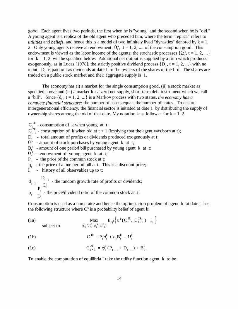
14

good. Each agent lives two periods, the first when he is "young" and the second when he is "old." A young agent is a replica of the old agent who preceded him, where the term "replica" refers toutilities and beliefs, and hence this is a model of two infinitely lived "dynasties" denoted by k = 1,2. Only young agents receive an endowment 6 , t = 1, 2, .... of the consumption good. Thist

k

endowment is viewed as the labor income of the agents; the stochastic processes {6 , t = 1, 2, ...} tk

for k = 1, 2 will be specified below. Additional net output is supplied by a firm which producesexogenously, as in Lucas [1978], the strictly positive dividend process {D , t = 1, 2, ...} with not

input. D is paid out as dividends at date t to the owners of the shares of the firm. The shares aret

traded on a public stock market and their aggregate supply is 1.

The economy has (i) a market for the single consumption good, (ii) a stock market asspecified above and (iii) a market for a zero net supply, short term debt instrument which we calla "bill". Since {d , t = 1, 2, ...} is a Markov process with two states, the economy has at

complete financial structure: the number of assets equals the number of states. To ensureintergenerational efficiency, the financial sector is initiated at date 1 by distributing the supply ofownership shares among the old of that date. My notation is as follows: for k = 1, 2

- consumption of k when young at t; - consumption of k when old at t + 1 (implying that the agent was born at t);

D - total amount of profits or dividends produced exogenously at t;t

� - amount of stock purchases by young agent k at t;tk

B - amount of one period bill purchased by young agent k at t;t k

6 - endowment of young agent k at t;tk

P - the price of the common stock at t;t

- the price of a one period bill at t. This is a discount price;I - history of all observables up to t;t

- the random growth rate of profits or dividends;

- the price/dividend ratio of the common stock at t;

Consumption is used as a numeraire and hence the optimization problem of agent k at date t hasthe following structure where Q is a probability belief of agent k:k

(1a)subject to

(1b)

(1c)

To enable the computation of equilibria I take the utility function agent k to be

uk(C1kt , C2k

t � 1 ) 1

1 �k

(C1kt ) 1 �k

�

�k

1 �k

(C2kt � 1) 1 �k , �k > 0 , 0 <�k < 1.

Pt(C1kt )

�k� �k EQ k

t( (C2k

t � 1)�k (Pt�1�Dt�1) | It ) 0

qt(C1kt )

�k� �k EQ k

t( (C2k

t � 1)�k | It ) 0 .

Dt � 1 Dtdt � 1

1 , 1 11 1 , 1

7kt

6kt

Dt

b kt

B kt

Dt

c1kt

C1kt

Dt

c2kt�1

C2kt�1

Dt�1

D1 �k

t D�k

t

c 1kt pt�

kt qt b

kt � 7

k

c2kt�1 �

kt (pt�1� 1) �

b kt

dt�1

pt(c1kt )

�k� �kEQ k

t( (c2k

t�1dt�1)�k (pt�1�1)dt�1) | It ) 0

qt(c1kt )

�k� �k EQ k

t( (c2k

t � 1dt � 1)�k | It ) 0

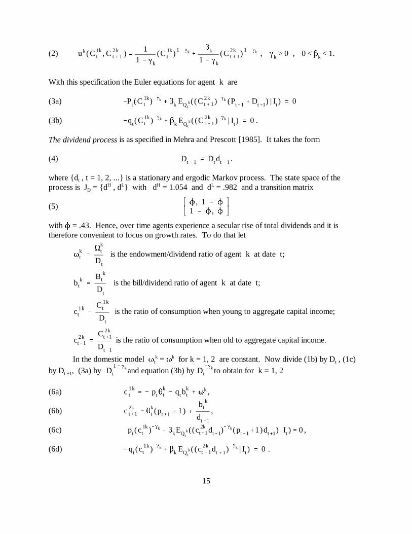
15

(2)

With this specification the Euler equations for agent k are

(3a)

(3b)

The dividend process is as specified in Mehra and Prescott [1985]. It takes the form

(4) .

where {d , t = 1, 2, ...} is a stationary and ergodic Markov process. The state space of thet

process is J = {d , d } with d = 1.054 and d = .982 and a transition matrixDH L H L

(5)

with 1 = .43. Hence, over time agents experience a secular rise of total dividends and it istherefore convenient to focus on growth rates. To do that let

is the endowment/dividend ratio of agent k at date t;

is the bill/dividend ratio of agent k at date t;

is the ratio of consumption when young to aggregate capital income;

is the ratio of consumption when old to aggregate capital income.

In the domestic model 7 = 7 for k = 1, 2 are constant. Now divide (1b) by D , (1c)t tk k

by D , (3a) by and equation (3b) by to obtain for k = 1, 2 t +1

(6a) ,

(6b) ,

(6c) ,

(6d) .

bkt bk

t (pt , qt , dt , It )

�kt �

kt (pt , qt , dt , It )

�1t � �

2t 1

b1t � b 2

t 0

(pt�1,qt�1,dt�1,ykt�1) (pt , qt , dt , yk

t )

bkt bk(pt , qt , dt , yk

t )

�kt �k(pt , qt , dt , yk

t )

16

The optimum conditions (6a) - (6d) imply the following demand functions for k = 1, 2

(7a) ,

(7b) .

Equilibrium requires the market clearing conditions

(7c)

(7d) ;

The equilibrium implied by (7a)-(7d) depends upon the beliefs of the agents. I studyMarkov equilibria with a finite number of prices. An equilibrium is characterized either by oneMarkov matrix or by a sequence of such matrices which describe the transition from a price stateto another. However, the stationary measure m will be described by a single transition matrixfrom prices at t to prices at t + 1 which I call . The two agents hold rational beliefs Q k

which are stable Markov probabilities with stationary measures defined by . It is clear that therationality of belief conditions can be very complicated. The technique of "assessment variables"is the main technical development in Nielsen [1996] and Kurz and Schneider [1996]. It enables asimple description of a large family of rational beliefs.

III(A.2) Rational Belief Equilibrium. Assessment variables of agents are sequences of randomvariables {y , t = 1, 2, ...} for k = 1, 2 and here I assume that y � Y = {0, 1}. The belief oft t

k k

agent k is a probability Q over the joint process {(p ,q , d , y ), t = 1, 2, ...} which is ak kt t t t

Markov process. The decision functions in (6a) - (6d) are selected based on the conditionalprobability of Q given the value of y .k k

t

As a matter of economic interpretation, assessment variables are parameters indicatinghow an agent perceives the state of the economy and are thus tools for the description of stableand non-stationary processes. In the model at hand they are the method of describing if an agent isoptimistic or pessimistic at date t about capital gains at date t + 1. I thus need to clarify howassessment variables enter the decision mechanism of agent k. Note that in (6c) - (6d) agent k specifies the probability of conditional on - the value ofhis assessment variable jointly with the observed data. It then follows from the Markovassumptions that the demand functions of agent k for stocks and bills are functions of the form

(10a)

(10b) .

Consequently the market clearing conditions are

(dt , y1t , y2

t )

�1(pt , qt , dt , y1t ) � �2(pt , qt , dt , y2

t ) 1

b1(pt , qt , dt , y1t ) � b 2(pt , qt , dt , y2

t ) 0 .

pt

qt 0�(dt , y1

t , y2t )

(y 1t , y2

t ) y kt � {0 , 1} y k

t 1y k

t 0(y1

t , y2t )

(pt , qt )(dt , y1

t , y2t )

(pt , qt ) (pt�1 , qt�1)(dt , y1

t , y2t ) (dt�1 , y1

t�1 , y2t�1)

(dt , y1t , y2

t )(pt , qt )

(pt , qt ) (pt�1, qt�1)

(pt , qt )(pt�1 , qt�1)

y kt y k

t 1

The choice of the equilibrium dynamics being generated by a fixed, stationary matrix is a matter of6

convenience and simplicity . The process { , t = 1, 2, ...} could have been selected to be anystable process with a Markov stationary measure induced by the empirical distribution. In such a case thefixed transition matrix would characterize only the stationary measure of the equilibrium dynamics ratherthan be the matrix of the true probability of the equilibrium dynamics of prices.

17

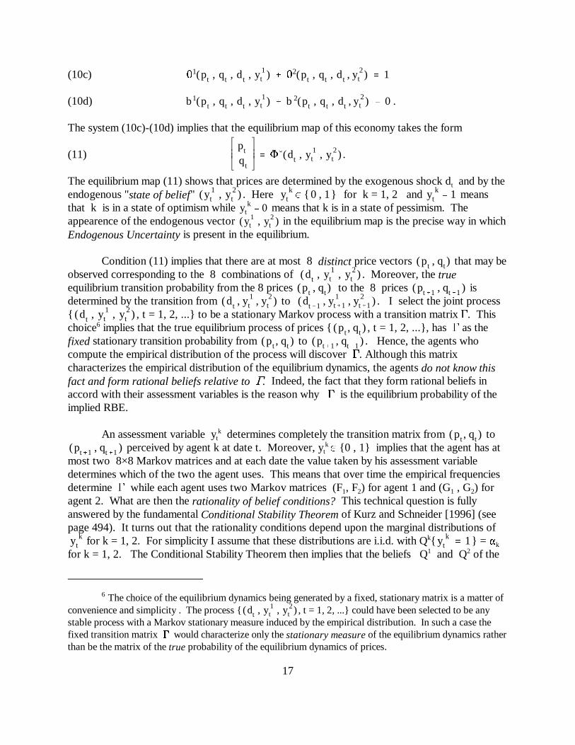
(10c)

(10d)

The system (10c)-(10d) implies that the equilibrium map of this economy takes the form

(11) .

The equilibrium map (11) shows that prices are determined by the exogenous shock d and by thet

endogenous "state of belief" . Here for k = 1, 2 and meansthat k is in a state of optimism while means that k is in a state of pessimism. Theappearence of the endogenous vector in the equilibrium map is the precise way in whichEndogenous Uncertainty is present in the equilibrium.

Condition (11) implies that there are at most 8 distinct price vectors that may beobserved corresponding to the 8 combinations of . Moreover, the trueequilibrium transition probability from the 8 prices to the 8 prices isdetermined by the transition from to . I select the joint process{ , t = 1, 2, ...} to be a stationary Markov process with a transition matrix . Thischoice implies that the true equilibrium process of prices { , t = 1, 2, ...}, has as the6

fixed stationary transition probability from to . Hence, the agents whocompute the empirical distribution of the process will discover . Although this matrixcharacterizes the empirical distribution of the equilibrium dynamics, the agents do not know thisfact and form rational beliefs relative to . Indeed, the fact that they form rational beliefs inaccord with their assessment variables is the reason why is the equilibrium probability of theimplied RBE.

An assessment variable y determines completely the transition matrix from totk

perceived by agent k at date t. Moreover, y� {0 , 1} implies that the agent has attk

most two 8×8 Markov matrices and at each date the value taken by his assessment variabledetermines which of the two the agent uses. This means that over time the empirical frequenciesdetermine while each agent uses two Markov matrices (F , F ) for agent 1 and (G , G ) for1 2 1 2

agent 2. What are then the rationality of belief conditions? This technical question is fullyanswered by the fundamental Conditional Stability Theorem of Kurz and Schneider [1996] (seepage 494). It turns out that the rationality conditions depend upon the marginal distributions of

for k = 1, 2. For simplicity I assume that these distributions are i.i.d. with Q { } = �kk

for k = 1, 2. The Conditional Stability Theorem then implies that the beliefs Q and Q of the1 2

�1F1 � (1 �1)F2 , �2G1 � (1 �2)G2

(y 1t , y2

t )

(pt�1, qt�1, dt�1)

18

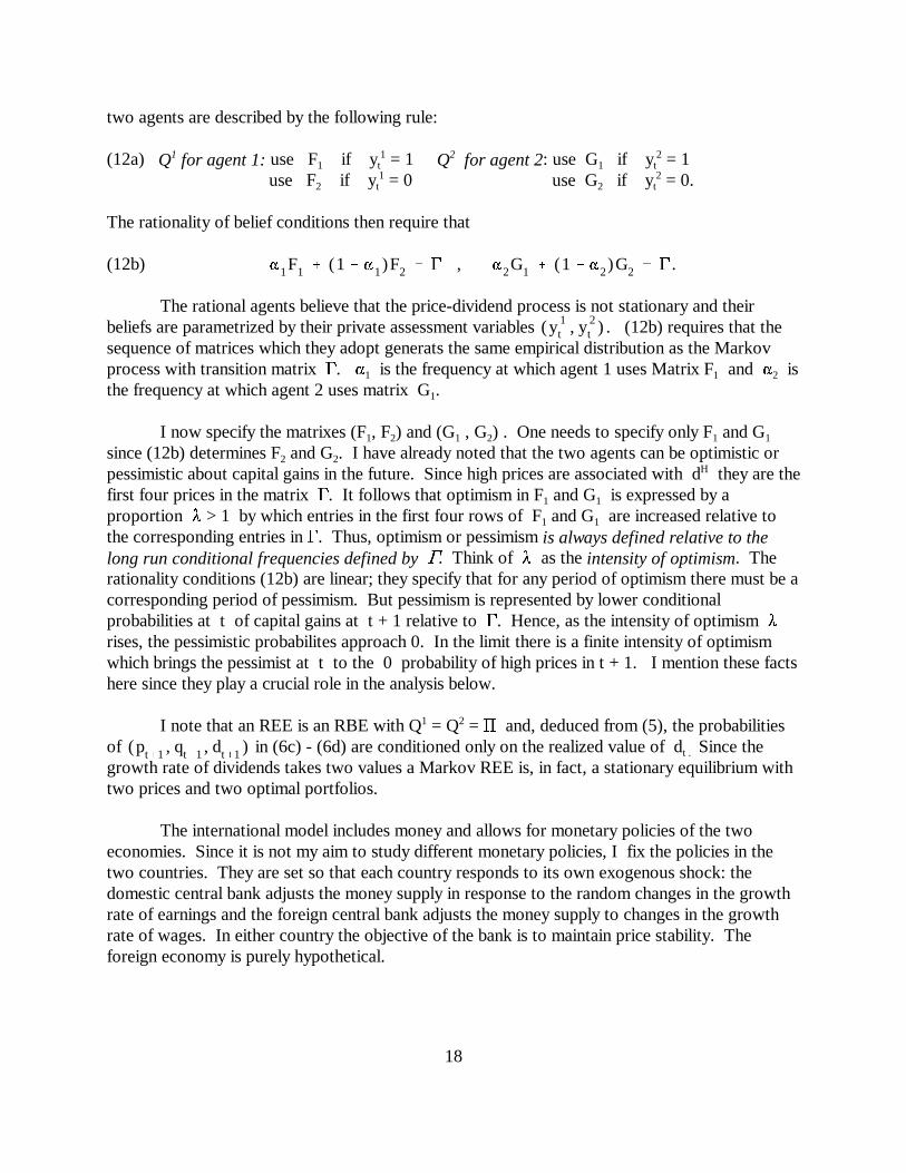
two agents are described by the following rule:

(12a) Q for agent 1: use F if y = 1 Q for agent 2: use G if y = 11 1 2 21 t 1 t

use F if y = 0 use G if y = 0.2 t 2 t1 2

The rationality of belief conditions then require that

(12b) .

The rational agents believe that the price-dividend process is not stationary and theirbeliefs are parametrized by their private assessment variables . (12b) requires that thesequence of matrices which they adopt generats the same empirical distribution as the Markovprocess with transition matrix . � is the frequency at which agent 1 uses Matrix F and � is1 1 2

the frequency at which agent 2 uses matrix G .1

I now specify the matrixes (F , F ) and (G , G ) . One needs to specify only F and G 1 2 1 2 1 1

since (12b) determines F and G . I have already noted that the two agents can be optimistic or2 2

pessimistic about capital gains in the future. Since high prices are associated with d they are theH

first four prices in the matrix . It follows that optimism in F and G is expressed by a1 1

proportion � > 1 by which entries in the first four rows of F and G are increased relative to1 1

the corresponding entries in . Thus, optimism or pessimism is always defined relative to thelong run conditional frequencies defined by . Think of � as the intensity of optimism. Therationality conditions (12b) are linear; they specify that for any period of optimism there must be acorresponding period of pessimism. But pessimism is represented by lower conditionalprobabilities at t of capital gains at t + 1 relative to . Hence, as the intensity of optimism � rises, the pessimistic probabilites approach 0. In the limit there is a finite intensity of optimismwhich brings the pessimist at t to the 0 probability of high prices in t + 1. I mention these factshere since they play a crucial role in the analysis below.

I note that an REE is an RBE with Q = Q = $ and, deduced from (5), the probabilities1 2

of in (6c) - (6d) are conditioned only on the realized value of d Since thet .

growth rate of dividends takes two values a Markov REE is, in fact, a stationary equilibrium withtwo prices and two optimal portfolios.

The international model includes money and allows for monetary policies of the twoeconomies. Since it is not my aim to study different monetary policies, I fix the policies in thetwo countries. They are set so that each country responds to its own exogenous shock: thedomestic central bank adjusts the money supply in response to the random changes in the growthrate of earnings and the foreign central bank adjusts the money supply to changes in the growthrate of wages. In either country the objective of the bank is to maintain price stability. Theforeign economy is purely hypothetical.

19

III(B) On the Method of Simulations.What is the logic of a simulation model and why should we consider this method of

analysis valid? To answer this question I note first that the parameters of the real economy areselected so as to conform to well known parameters of econometric models that were estimatedfor the U.S. economy. These include the long term growth rates of wages and earnings and thecoefficients of risk aversion and discount rates of the agents. As a result, the real part of theeconomy is required to act in conformity with what we know about the long run tendencies of theU.S. economy. Hence, the fundamentals of the economy are exactly the same as we know fromthe statistics of the real economy. The parameters which I, as a model builder, will select arethose that relate to the beliefs of the agents and their distributions. The simulation models thenask what would be the implications of alternative belief structures for price volatility, holding thefundamentals fixed. Since rational expectations are among the beliefs which can be examined inthe model, the results below will provide a comparison between the implications of rationalexpectations and rational beliefs for price volatility, keeping the real economy the same.

It has been well documented that if one imposes on the real fundamentals of the simulationmodels the assumption of rational expectations by the agents, all the problems and paradoxesspecified earlier will appear and I shall demonstrate that this remains true in the models at hand. However, if I can show that under the assumption that the agents hold rational beliefs the financialmarkets will not exhibit any of the paradoxes, then it follows that the belief structure of the agentsdoes provide a unified paradigm to resolve the specified problems. It would then be useful tohave an intuitive understanding of the structure of beliefs that generate the various conclusionsand I will attempt to provide some interpretation in a later section.

The foreign economy is a purely hypothetical economy; it is not calibrated to anyparticular economy. The two economies will have a common ("world") stock market and theforeign economy will have an exogenous endowment shock.

III(C) Simulation Demonstration of the Solutions to the Four ProblemsIn the Tables below I present comparisons between the simulation results under rational

expectations and under rational beliefs. The aim is first to exhibit what are the problems whicharise under REE and then to show that these problems are significantly resolved under the unifiedparadigm of the theory of rational beliefs. The sequence of the tables below correspond to thequestions posed at the start.

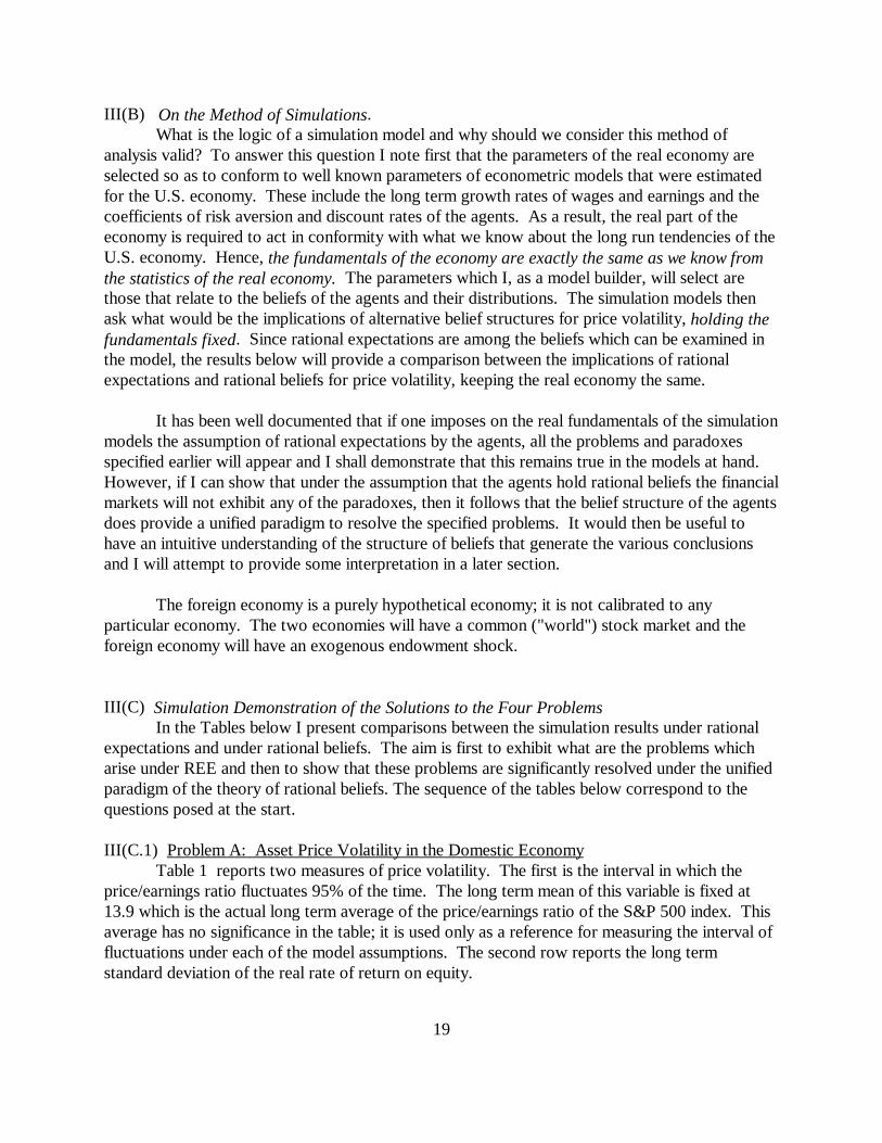
III(C.1) Problem A: Asset Price Volatility in the Domestic EconomyTable 1 reports two measures of price volatility. The first is the interval in which the

price/earnings ratio fluctuates 95% of the time. The long term mean of this variable is fixed at13.9 which is the actual long term average of the price/earnings ratio of the S&P 500 index. Thisaverage has no significance in the table; it is used only as a reference for measuring the interval offluctuations under each of the model assumptions. The second row reports the long termstandard deviation of the real rate of return on equity.

)r

r F

'

20

Table 1: Long Run Volatility of the Price/Earnings Ratio and the Return on Equity

Under Rational Under Rational ActualExpectations Beliefs

Interval in which the price/earnings ratio fluctuates 95% of the time [ 13.8 , 14.0 ] [ 9.4 , 18.4 ] [ 5.5 , 22.3]

- the long term standard deviation of 4.1% 17.5% 18.4%the return on equity

The table exhibits the problem which arises under rational expectations: if stock pricesvary strictly in accord with fundamentals they would not change very much! The variance of theprice/earning ratio is bigger by an order of magnitude under rational beliefs than under rationalexpectations. The table shows that under rational beliefs the index would have spent 95% of thetime between 9.4 and 18.4 which is of the same order of magnitude as the historical record. Thisinterval is somewhat smaller than the actual interval reported in the last column, a fact that may beexplained by the generally agreed upon observation that the fluctuations of the reportedprice/earnings ratio are sensitive to tax and accounting practices. These tend to overstate thevolatility of recorded earnings relative to the true economic earnings of the companies in theindex. The actual long term standard deviation of the return on the S&P 500 index is 18.4% andthe simulations under rational beliefs lead to a standard deviation of 17.5%. These two measuresof volatility are very close.

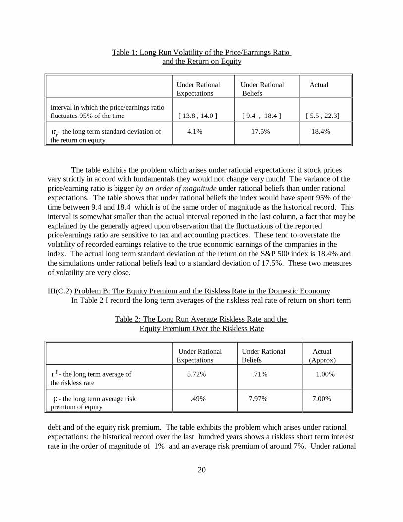
III(C.2) Problem B: The Equity Premium and the Riskless Rate in the Domestic Economy In Table 2 I record the long term averages of the riskless real rate of return on short term

Table 2: The Long Run Average Riskless Rate and the Equity Premium Over the Riskless Rate

Under Rational Under Rational ActualExpectations Beliefs (Approx)

- the long term average of 5.72% .71% 1.00%the riskless rate

- the long term average risk .49% 7.97% 7.00%premium of equity

debt and of the equity risk premium. The table exhibits the problem which arises under rationalexpectations: the historical record over the last hundred years shows a riskless short term interestrate in the order of magnitude of 1% and an average risk premium of around 7%. Under rational

21

expectations the model fails to come close to these facts. Under rational beliefs the averageequity premium is 7.97%, the average riskless rate is .71% and these figures correspond to thehistorical record.

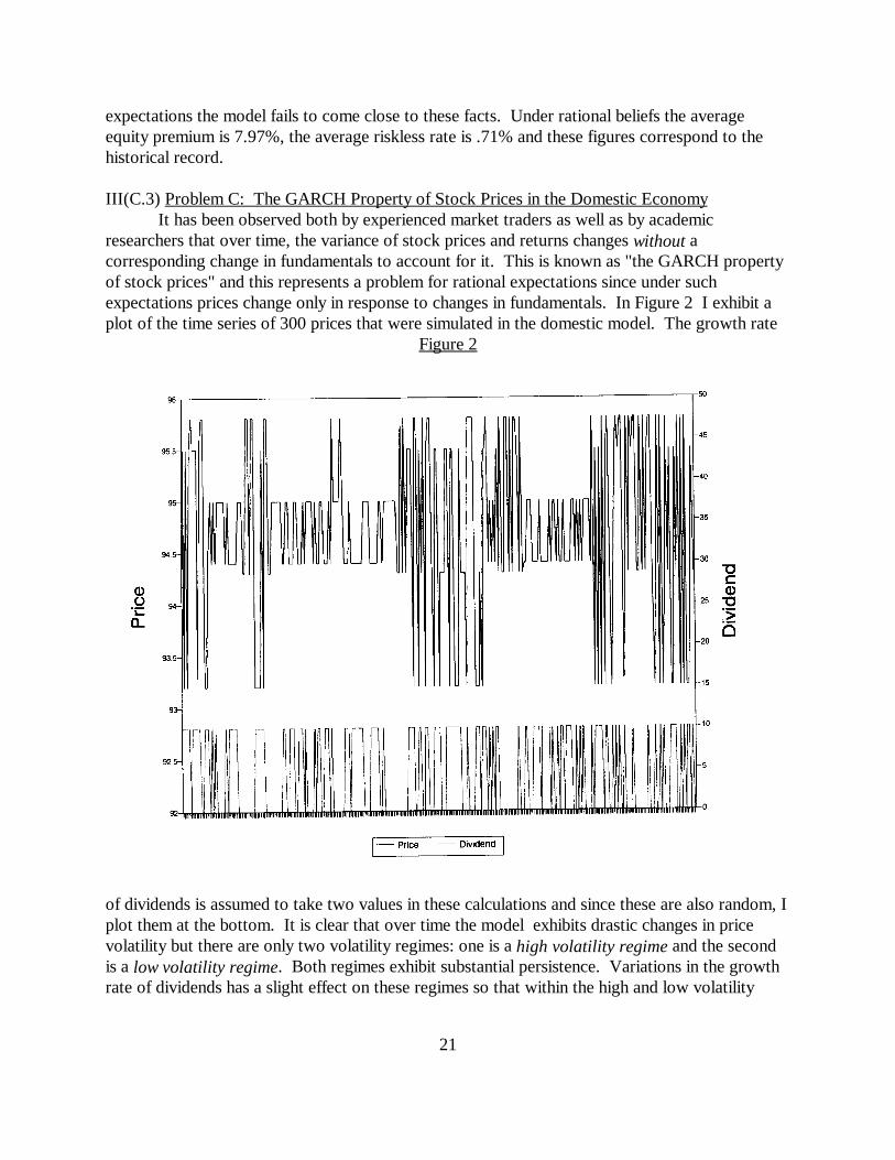
III(C.3) Problem C: The GARCH Property of Stock Prices in the Domestic EconomyIt has been observed both by experienced market traders as well as by academic

researchers that over time, the variance of stock prices and returns changes without acorresponding change in fundamentals to account for it. This is known as "the GARCH propertyof stock prices" and this represents a problem for rational expectations since under suchexpectations prices change only in response to changes in fundamentals. In Figure 2 I exhibit a plot of the time series of 300 prices that were simulated in the domestic model. The growth rate

Figure 2

of dividends is assumed to take two values in these calculations and since these are also random, Iplot them at the bottom. It is clear that over time the model exhibits drastic changes in pricevolatility but there are only two volatility regimes: one is a high volatility regime and the secondis a low volatility regime. Both regimes exhibit substantial persistence. Variations in the growthrate of dividends has a slight effect on these regimes so that within the high and low volatility

ext�1 ext

ext

c � � (rDt rF

t ) � Jt�1

(ext�1 ext )(rD

t rFt )

22

regimes there are sub-regimes whose volatility depends to a small degree upon dividends.

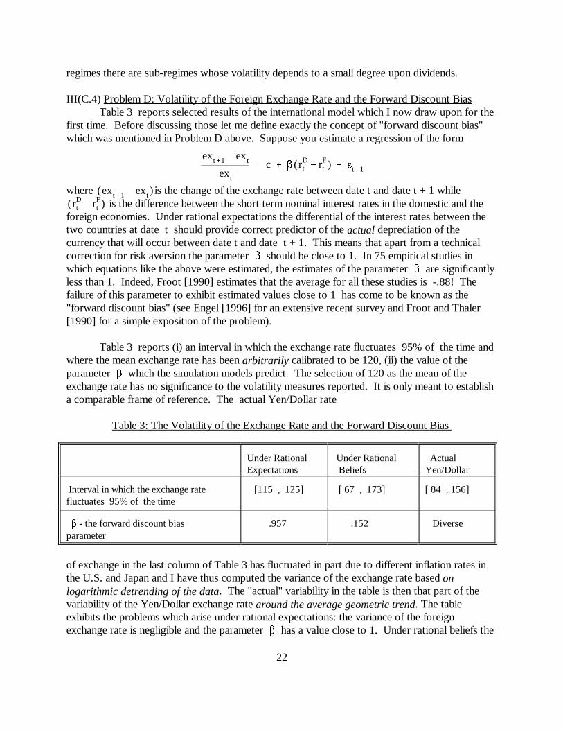
III(C.4) Problem D: Volatility of the Foreign Exchange Rate and the Forward Discount Bias Table 3 reports selected results of the international model which I now draw upon for the

first time. Before discussing those let me define exactly the concept of "forward discount bias"which was mentioned in Problem D above. Suppose you estimate a regression of the form

where is the change of the exchange rate between date t and date t + 1 while is the difference between the short term nominal interest rates in the domestic and the

foreign economies. Under rational expectations the differential of the interest rates between thetwo countries at date t should provide correct predictor of the actual depreciation of thecurrency that will occur between date t and date t + 1. This means that apart from a technicalcorrection for risk aversion the parameter � should be close to 1. In 75 empirical studies inwhich equations like the above were estimated, the estimates of the parameter � are significantlyless than 1. Indeed, Froot [1990] estimates that the average for all these studies is -.88! Thefailure of this parameter to exhibit estimated values close to 1 has come to be known as the"forward discount bias" (see Engel [1996] for an extensive recent survey and Froot and Thaler[1990] for a simple exposition of the problem).

Table 3 reports (i) an interval in which the exchange rate fluctuates 95% of the time andwhere the mean exchange rate has been arbitrarily calibrated to be 120, (ii) the value of theparameter � which the simulation models predict. The selection of 120 as the mean of theexchange rate has no significance to the volatility measures reported. It is only meant to establisha comparable frame of reference. The actual Yen/Dollar rate

Table 3: The Volatility of the Exchange Rate and the Forward Discount Bias

Under Rational Under Rational Actual Expectations Beliefs Yen/Dollar

Interval in which the exchange rate [115 , 125] [ 67 , 173] [ 84 , 156]fluctuates 95% of the time

� - the forward discount bias .957 .152 Diverse parameter

of exchange in the last column of Table 3 has fluctuated in part due to different inflation rates inthe U.S. and Japan and I have thus computed the variance of the exchange rate based onlogarithmic detrending of the data. The "actual" variability in the table is then that part of thevariability of the Yen/Dollar exchange rate around the average geometric trend. The tableexhibits the problems which arise under rational expectations: the variance of the foreignexchange rate is negligible and the parameter � has a value close to 1. Under rational beliefs the

23

results are drastically different: the variance of the foreign exchange is of the order of magnitudeof observed fluctuations in the market. Finally, the forward discount bias parameter in the RBEreported in the table is .152 which is significantly less than 1. Within the class of models usedhere a negative parameter could not be predicted.

IV. Simple Explanations of How the Theory Resolves Each of the Four Problems

In Section III I demonstrated that the unified paradigm offered by the theory of rationalbelief equilibrium (RBE) goes a long way towards solving the four problems that could not besolved within the prevailing rational expectations paradigm. In this section I will offer a simplebut systematic explanation of the results presented in Section III. In doing so I will alsodemonstrate the workings of the model of RBE.

(i) Volatility of Prices and Exchange Rates. The explanation of why the volatility of prices andexchange rates in an RBE exceed the level determined by the exogenous fundamentals of theeconomy is simple. Each agent forms his own theory of what the future will bring and thedistribution of the private models in the economy constitutes the "social state of belief." Variability in the state of belief in the market is then an important factor, together with theexogenous shocks, in explaining price volatility. Since the social state of belief is not observablewe need to seek proxies for it. Incomplete proxies can be seen in the distribution of priceforecasts announced by different forecasters in the market. Interesting distributions of short termand long term interest rate forecasts by professional economists are also revealing since all use thesame data. Thus the "state of belief" in the market is simply a "distribution of beliefs".

Endogenous uncertainty is then that component of price volatility which is caused by thedistribution of beliefs of the agents. Therefore, equilibrium price volatility can be represented as asum of the form

Market Uncertainty = Exogenous Uncertainty + Endogenous Uncertainty

Since exogenous uncertainty is that component of market volatility which is determined by thevolatility of the exogenous fundamental conditions in the market, it is then clear why total marketvolatility exceeds the level justified by fundamentals.

Without introducing technical details I stress that endogenous uncertainty has a dual effecton market volatility. One component of endogenous uncertainty is the amplification of the effectof fluctuations of exogenous fundamentals on price volatility. This is the effect whereby thedistribution of beliefs in the market can cause changes in the fundamental exogenous variables tohave a larger effect on price volatility than would be true in a corresponding rational expectationsequilibrium. The second component of endogenous uncertainty arises from the fact thatvariations in the distribution of beliefs cause additional pure price volatility which is uncorrelatedwith any fundamental information. This component of endogenous uncertainty may have

24

dramatic effects on the volatility of prices in an RBE since this component turns out to be affectedby correlation and commonality of beliefs among traders. When a large number of agents becomeoptimistic about capital gains, prices may rise. Conversely, when a large number of agentsbecome pessimistic prices decline.

The amplification component of Endogenous Uncertainty provides a natural explanation of thephenomenon which is recognized as "market overshooting." This is usually a reference to the factthat when prices are high they often proceed to go higher than can be justified by fundamentalsand when they go low, they go lower than can be justified by the exogenous variables. Naturally,excess volatility and overshooting is part of the historical record and is incorporated in theempirical distribution of any market. Hence it becomes part of the belief structure of agents: theyexpect the market to overshoot.

(ii) The Forward Discount Bias in foreign exchange rates. To see why this bias arises naturally inan RBE recall the rational expectations argument in favor of � = 1 (apart from the correction forrisk aversion which I ignore here). Hence, in such an equilibrium it is a theoretical conclusionthat the difference between the one period nominal rates in the two countries at date t is exactlyequal to the expected percentage depreciation of the exchange rate between the two currenciesbetween dates t and t + 1. This expectational arbitrage argument implies that in the realeconomy the differential between the one period nominal rates in the two countries will be anunbiased statistical forecast of the one period depreciation of the exchange rate in the next period. Under this proposition one would expect to have a regression coefficient of 1 between thepercentage differential of the nominal rates at date t and the actual percentage change of theexchange rate between dates t and t + 1.

The theory of RBE predicts that agents holding rational beliefs may make significantforecasting mistakes. This would result in a true, equilibrium, process of the exchange rate whichwould fluctuate excessively in part due to these mistaken forecasts. Hence, at almost no datewould the nominal interest differential between the two countries be an unbiased estimate of therate of depreciation of the exchange rate one period later and under such circumstances oneshould not expect the regression coefficient to be close to one. Agents who want to takeadvantage of such a regression, basing their investment strategy on a nominal rate differentialwhich appears to offer an investment opportunity, will find that this is not arbitrage in thestandard riskless sense of the term. At date t the exchange rate at date t + 1 is a randomvariable. In an RBE any trade on the spread between the nominal interest rates of two curenciesrequires agents to take a foreign exchange risk which is valued different by agents holding diversebeliefs.

Should we expect that under rational beliefs the parameter � satisfies � < 1? The answeris yes for the following reason. Consider first a rational expectations equilibrium in which thedifference between the domestic and foreign nominal interest rates is z%. In that equilibrium youdo not need to form expectations on the currency depreciation itself. It is sufficient for you tobelieve that other investors or currency arbitrageurs know the true probability of currency

For more details about the nature of GARCH and related processes see Bollerslev, Chou and6

Kroner [1992] and Bollerslev, Engle and Nelson [1994].

25

depreciation and they have already induced the interest differential to be equal to the average rateof currency depreciation which will be z%. Now consider an RBE. All agents know that no oneknows the true probability distribution of the exchange rate and therefore the exchange rate issubject to endogenous uncertainty. Being risk averse, agents who invest in foreign currencywould demand a risk premium on endogenous uncertainty and over the long run the difference (1-�) is the premium received by currency speculators for being willing to carry foreign currencypositions. For a positive premium it follows that � < 1.

(iii) The GARCH Property of Asset Prices. As indicated earlier, the states of belief of different6

individual investors may be highly correlated and this is a consequence of the many modes ofcommunication in our society. Investors talk to each other and this interaction causes them toinfluence each other; they all read the same newspapers, the same reports of the Wall Streetanalysts and watch the same television programs which feature expert views on the economicconditions in the future. Analysts and experts know each other, they talk to each other and attendthe same conferences thus tend to correlate their views either in agreement or disagreement. Theconsequence of this correlation among the beliefs of agents is that the distribution of beliefs tendsto switch across different "cognitive" centers of gravity. Indeed, each such center of gravity is a"belief regime". The important examples of such regimes of belief are regimes of "consensus" and"non-consensus." The persistence of the states of belief is an important element in the emergenceof the GARCH property. In the models studied here the state of belief is a Markov process withdegrees of persistence which depend upon the parametrization of each model.

The emergence of the GARCH property is a consequence of two different effects whichthe distribution of beliefs has on the market. These two effects are directly related to the relativestrength of the two components of Endogenous Uncertainty discussed above: amplification andpure endogenous volatility. I will start with pure endogenous volatility since this effect is simpler. It turns out that what really matters for the effect of this component of endogenous volatility onthe emergence of the GARCH phenomenon is the persistence of the regime of consensus vs. theregime of market non consensus. A regime of market consensus is formed when the models ofthe majority of traders generate similar predictions and if the regime persists, then over time, if thereal economy remains in the same state ("high" for expansion and "low"for recession) the tradersmove together between states of optimism and states of pessimism. Such fluctuations betweenoptimistic and pessimistic outlooks on market prices may occur on many different frequencies. Non-consensus is a belief regime in which the distribution of models used by the agents isrelatively spread out and consequently their predictions vary widely across the different possibleoutcomes in the future. If the regime of non-consensus persists then, at a given state of the realeconomy, the diverse forecasts tend to cancel each other out over time.

I now observe that when the regime of consensus is formed the pure volatility component

26

of security prices will be high. This is so since all agents are either optimistic or pessimistic at thesame time; when optimistic they want to buy the same portfolio and when pessimistic they wantto sell the same portfolio leading to price volatility. Conversely, when a non-consensus regimeoccurs the opposite is true: the distribution of beliefs is one in which the excess demand of theoptimists matches the excess supply of the pessimists leading to low volatility. This component ofendogenous volatility is not correlated with real exogenous shocks.

I turn now to the effect of "amplification" which is drastically different from the firsteffect. To understand this second effect consider two different states of belief each of which has ahigh degree of persistence. For example, let the first state be one of "universal optimism" and thesecond state be one of "non-consensus" or "disagreement". Given the state of optimism, priceswill vary with the state of the dividend growth. However, assuming a strong endogenousamplification, prices will overreact to changes in the fundamental information but the degree ofamplification is not the same in the state of total optimism as in the state of non-consensus. Ifthe economy is in a state of optimism (and remains there) the variations in asset prices due tocyclical output fluctuations is usually relatively small so that the variance of prices in that state isrelatively small. If the economy is in the state of non-consensus (and remains there) the priceresponse to cyclical output fluctuations is very different depending upon the intensity of optimismand pessimism. As we shall see later, in all models presented here the pessimists are more intensethan the optimists. Consequently, if in a state of non-consensus the net output state is "low" (i.e.recession) then the pessimists will dominate by making the price crash even further but if the stateis "high" the pessimistic outlook has less force and prices will rebound sharply. As a result, thevariance of prices in that state is very high. In short, as the economy moves among differentstates of belief the level of asset prices will change, but more importantly, the variance of priceswill vary, giving rise to the GARCH property.

To generalize these conclusions beyond the simulation models, the theory of RBE showsthat the variance of stock prices depends upon the distribution of beliefs in the market and sincethis distribution changes over time, so does the variance of stock prices. Also, in an RBE agentscan utilize exogenous shocks and realized prices to determine their state of belief about the future. Consequently, the distribution of beliefs and hence the variance of prices may depend upon boththe correlation among the beliefs of the agents as well as the exogenous shocks and realizedprices. Both of these may change abruptly, and so can the induced regime of beliefs.

The models used in the simulations relate to events which occur over long stretches oftime and hence the simulation results apply to low frequencies (i.e. months and years). These donot address the structure of volatility at high frequencies investigated by some papers of theGARCH literature (see for example Bollerslev, Chou and Kroner [1992] and Brock and LeBaron[1996]). This limitation of the results here should not obscure the main conclusion to which thetheory of RBE leads: the GARCH phenomenon is caused both by the persistence as well as by theabrupt shifts in the distribution of beliefs. These forces hold over low or high frequencies.

The debate regarding "The Equity Premium Puzzle" was initiated by Mehra and Prescott [1985]. A7

sample of other papers on the subject include Mankiw [1986], Reitz [1988], Weil [1989], Epstein and Zin[1990], Constantinides [1990], Campbell and Cochrane [1999], Brennan and Xia [1998] and Abel [1999].

27

(iv) The Equity Premium and the Riskless Rate. Explaining the factors which determine the7

equity risk premium (i.e. "the" premium) in an RBE is ultimately simple but demands the reviewof the technical conditions which formulate the rationality of beliefs of the agents. A direct andsimple explanation flows naturally from the resolution of Problem A. It proposes that in an RBEendogenous uncertainty causes the total level of uncertainty to exceed the level that would prevailunder rational expectations. Risk averse investors would then demand a higher risk premium forholding equity which is more risky in an RBE than in a rational expectations equilibrium and forthat reason the premium would be higher in an RBE. This explanation has a grain of truth butneeds to be qualified by two additional considerations.

The first consideration suggests that due to the diversity of beliefs the equity premiumarises in a world where optimists and pessimists reside together. The risk premium demanded byoptimists is likely to be different from the premium demanded by pessimists and hence, the marketpremium must depend upon the distribution of beliefs. Indeed, there are proportions of optimistsand pessimists which do not generate a higher equity risk premium than is generated underrational expectations. Second, an important component of the equity premium puzzle has beenthe question of why the riskless rate predicted by rational expectations models has been so muchhigher than the mean riskless rate realized over the last century and this question must be clearedas well. The direct explanation given above does not address the question of why the riskless rateis so much lower in the simulated RBE relative to rational expectations equilibria.

To gain intuition into the two issues above I must bring you into some of the moretechnical aspects of the theory and to do that I examine a very simple model (based on Kurz[1998]). Consider an economy with two types (� and �) of agents who are different only in theirmodels of market price behavior (i.e. their beliefs). As part of their models, each of the type �agents has an assessment and when the assessment takes the value 1 the agent uses probabilitydistribution F of future prices and when it takes the value 2 the agent uses probability distribution1

F . These assessment variables are different for the two types. For this reason I denote the2

probabilities used by type � agents by G when the assessment of a type � agent takes the value 11

and by G when the assessment of a type � agent takes the value 2. However, I also assume that2

there is a very large number of agents of each type and each of them has his own separateassessment. Now, the assessments of the large number of agents of each of the types are,statistically speaking, the same random variables since these agents are of the same type but nowcomes the deeper question: are these assessments independent random variables? To addressthis question I must take an indirect route.

Some who object to models with heterogenous beliefs have suggested that in a largeeconomy consisting of many agents with independent beliefs the law of large numbers wouldoperate to average out the diversity of beliefs. Such averaging should render the model of diverse

28

beliefs irrelevant, leading the model of a large economy to function like a model of therepresentative household with a single, rational expectations belief. This intuitive argument ismisleading and the reasons are the key to understanding why a large equity premium and a lowriskless rate can be generated in an RBE.

Let me then return to my simple model and make the strong assumption that all theassessments within each type are i.i.d. with the probability of assessment taking the value of 1 being, say, .60. The consequence of this assumption is that although the probability used by anyone agent depends upon his assessment, the distribution of beliefs in the economy is fixed at ((.60, .40), (.60, .40)). That is, at all times 60% of type � agents use probability distribution F1

and 40% of them use F . A similar situation is assumed with respect to type � agents. If I now2

interpret F and G to mean "optimistic beliefs about higher returns next period" and F and G to1 1 2 2

mean "pessimistic beliefs about higher returns next period" then I have an economy where the lawof large number holds as required. At all times the distribution of beliefs is constant with 60% ofeach type optimistic and 40% pessimistic. The terms "optimism" and "pessimism" are exactly thesame proportions defined before and hence I will call these proportions (which are fixed for eachtype but may be different across the two types ) the "intensities of optimism" or the "intensities ofpessimism". I use the term "intensities" rather than "intensity" since these intensities of optimismor pessimism may vary depending upon current prices.

In this economy 60% of the agents are always optimistic, using F or G , and hence each1 1

agent fluctuates between optimistic and pessimistic outlooks with a frequency of .60 in theoptimistic mode and a frequency of .40 in the pessimistic mode. This would make sense onlywhen I consider the rationality of belief conditions which the agents satisfy. These stipulate thatthe beliefs may fluctuate over time but must average to . The RBE is then established if type �agents satisfy the condition .60F + .40F = and type � agents satisfy condition .60G +1 2 1

.40G = . But now I need to compare two equilibria: an REE in which all the agents hold the2

belief and the RBE in which 60% are optimists and 40% are pessimists relative to . Thoseclaiming that independent beliefs do not matter would propose that these two equilibria are thesame in the sense that prices and allocations are the same. I will show that these two are verydifferent equilibria with drastically different equity premia and volatility characteristics.

To convince you of that fact suppose that the initial percentage of pessimists in theeconomy is x = .40 and in equilibrium the rationality condition (1 - x)F + xF = is satisfied. 1 2

Now I lower the percentage x = .40 to x1. Would the rationality of belief condition (1 -x1)F1

+ x1 F = be satisfied with x1? The answer is no since my decrease of the percentage of2

pessimists from x = .40 to x1 without changing the matrices (F , F , G , G ) means that I1 2 1 2

reduced the weight assigned to the pessimistic matrix F and increased the weight assigned to the2

optimistic matrix F leading to the result that (1 -x1)F + x1 F g . Hence, as the number of1 1 2

pessimists in the market declines, I must adjust the intensity parameters in F and in G so that2 2

the intensity of their pessimism increases. Indeed, a point will be reached at which I could notlower the fraction of pessimists any further since the intensity of their pessimism has reached apoint where, given some price, they are virtually certain that they will lose money between date t

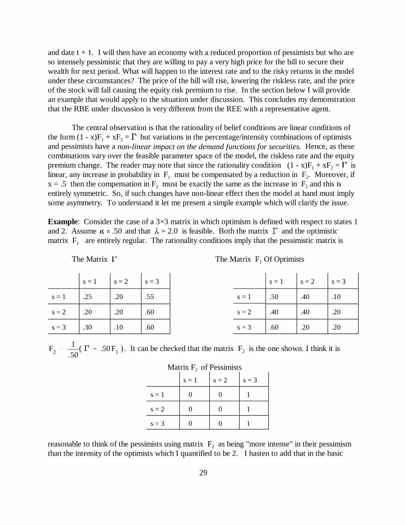
� .50

F2 1

.50( .50F1 )

29

and date t + 1. I will then have an economy with a reduced proportion of pessimists but who areso intensely pessimistic that they are willing to pay a very high price for the bill to secure theirwealth for next period. What will happen to the interest rate and to the risky returns in the modelunder these circumstances? The price of the bill will rise, lowering the riskless rate, and the priceof the stock will fall causing the equity risk premium to rise. In the section below I will providean example that would apply to the situation under discussion. This concludes my demonstrationthat the RBE under discussion is very different from the REE with a representative agent.

The central observation is that the rationality of belief conditions are linear conditions ofthe form (1 - x)F + xF = but variations in the percentage/intensity combinations of optimists1 2

and pessimists have a non-linear impact on the demand functions for securities. Hence, as thesecombinations vary over the feasible parameter space of the model, the riskless rate and the equitypremium change. The reader may note that since the rationality condition (1 - x)F + xF = is1 2

linear, any increase in probability in F must be compensated by a reduction in F . Moreover, if1 2

x = .5 then the compensation in F must be exactly the same as the increase in F and this is2 1

entirely symmetric. So, if such changes have non-linear effect then the model at hand must implysome asymmetry. To understand it let me present a simple example which will clarify the issue.

Example: Consider the case of a 3×3 matrix in which optimism is defined with respect to states 1and 2. Assume and that � = 2.0 is feasible. Both the matrix and the optimisticmatrix F are entirely regular. The rationality conditions imply that the pessimistic matrix is 1

The Matrix The Matrix F Of Optimists1

s = 1 s = 2 s = 3 s = 1 s = 2 s = 3

s = 1 .25 .20 .55 s = 1 .50 .40 .10

s = 2 .20 .20 .60 s = 2 .40 .40 .20

s = 3 .30 .10 .60 s = 3 .60 .20 .20

. It can be checked that the matrix F is the one shown. I think it is 2

Matrix F of Pessimists2

s = 1 s = 2 s = 3

s = 1 0 0 1

s = 2 0 0 1

s = 3 0 0 1

reasonable to think of the pessimists using matrix F as being "more intense" in their pessimism2

than the intensity of the optimists which I quantified to be 2. I hasten to add that in the basic

� .57

See, for example, the papers by Brock [1993],[1996], Durlauf [1993],[1994] and Föllmer [1974].8

30

model discussed in this paper � = 2.0 is not feasible and the matrix needs to be compatiblewith (5) and for this reason does not have the simple structure as in the example. Indeed, in themodel above � = 1.7542 and .

Given the basic observation that at any date the risk premium is determined by theexogenous variables and by the distribution of beliefs in the market, I reexamine the assumptionsmade earlier. Recall that I have assumed that the assessments are i.i.d. in order to refute thecriticism that heterogeneity of beliefs is irrelevant in a large economy with independent beliefs. Extensive research conducted in recent years has shown that it takes very little local interactionamong agents in the market in order to remove the effect of the law of large numbers onequilibrium variables such as prices. More specifically, under small local interactions, equilibriumaggregate variables of a large economy act as random variables rather than as constants . Given8

the natural interaction among the agents in financial markets there is ample theoretical justificationfor assuming that the beliefs of agents in the market are correlated and hence their assessments arenot jointly i.i.d. On the empirical side, there is little data on the distribution of beliefs in themarket. However, the litle evidence which is available (such as the forecasts of analysts on WallStreet) suggests that individual beliefs are highly correlated. Hence, both theoretical as well asempirical considerations imply that we should study models where the distribution of beliefs is arandom variable, jointly distributed with prices and other equilibrium variables.

The argument developed earlier (for an economy with i.i.d. assessments) regarding thebelief intensity of the pessimists remains valid in an economy with correlation among theassessments of the agents. The only difference is that now the distribution of beliefs changes overtime and the riskless rate and equity premium vary with the states of the economy. Hence, theRBE model’s prediction of the long term averages of the riskless rate and of the equity premiumdepends now also upon the frequency at which the system visits those distributions of beliefswhich generate low riskless rate and high premium. As we consider patterns of correlation amongthe beliefs of agents we may also expand the range of empirical evidence that needs to beexplained. In this paper I considered only four variables which needed to be explained. In acomplete analysis of the equity premium one may ask for the model prediction to match otherempirical regularities. These would include:

(i) the first and second moments of the price\earning or price\dividend ratio;(ii) the first and second moments of the riskless rate on short term debt;(iii)the first and second moments of the risky return of equities;(iv)the equity premium.

The remarkable fact is that the basic model presented in this paper can explain all theseregularities simultaneously. In order to do that, the parametrization needs to be specified asfollows:

(i) the optimists need to constitute a majority of about 57%;(ii) the intensity of the optimists needs to be set at 1.7542 which is approximately themaximal rate feasible;

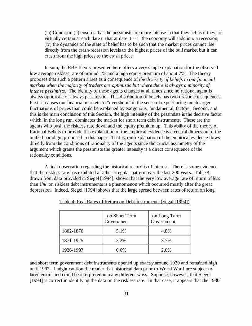
31

(iii) Condition (ii) ensures that the pessimists are more intense in that they act as if they arevirtually certain at each date t that at date t + 1 the economy will slide into a recession;(iv) the dynamics of the state of belief has to be such that the market prices cannot risedirectly from the crash-recession levels to the highest prices of the bull market but it cancrash from the high prices to the crash prices.

In sum, the RBE theory presented here offers a very simple explanation for the observedlow average riskless rate of around 1% and a high equity premium of about 7%. The theoryproposes that such a pattern arises as a consequence of the diversity of beliefs in our financialmarkets when the majority of traders are optimistic but where there is always a minority ofintense pessimists. The identity of these agents changes at all times since no rational agent isalways optimistic or always pessimistic. This distribution of beliefs has two drastic consequences. First, it causes our financial markets to "overshoot" in the sense of experiencing much largerfluctuations of prices than could be explained by exogenous, fundamental, factors. Second, andthis is the main conclusion of this Section, the high intensity of the pessimists is the decisive factorwhich, in the long run, dominates the market for short term debt instruments. These are theagents who push the riskless rate down and the equity premium up. This ability of the theory ofRational Beliefs to provide this explanation of the empirical evidence is a central dimension of theunified paradigm proposed in this paper. That is, our explanation of the empirical evidence flowsdirectly from the conditions of rationality of the agents since the crucial asymmetry of theargument which grants the pessimists the greater intensity is a direct consequence of therationality conditions.

A final observation regarding the historical record is of interest. There is some evidencethat the riskless rate has exhibited a rather irregular pattern over the last 200 years. Table 4,drawn from data provided in Siegel [1994], shows that the very low average rate of return of lessthan 1% on riskless debt instruments is a phenomenon which occurred mostly after the greatdepression. Indeed, Siegel [1994] shows that the large spread between rates of return on long

Table 4: Real Rates of Return on Debt Instruments (Segal [1994])

on Short Term on Long Term Government Government

1802-1870 5.1% 4.8%

1871-1925 3.2% 3.7%

1926-1997 0.6% 2.0%

and short term government debt instruments opened up exactly around 1930 and remained highuntil 1997. I might caution the reader that historical data prior to World War I are subject tolarge errors and could be interpreted in many different ways. Suppose, however, that Siegel[1994] is correct in identifying the data on the riskless rate. In that case, it appears that the 1930

32

depression has something to do with the low riskless rate. But such a fact provides furthersupport for the theory offered in this paper since this may establish the fact that the pessimists inmy RBE model based their pessimism on the experience of the 1930's. This does not mean thatthe probability which the pessimists attached to capital losses are exactly the empirical frequenciesof the great depressions. These empirical frequencies are part of the average historical record inthe matrix . Rationality of belief permits the pessimists to hold a probability F or G which2 2

do not correspond to any specific empirical frequency. However, it is the great depression thatmay have been responsible for the nature of the RBE which we have been discussing all along.

References

Abel, A.B. [1999], Risk Premia and Term Premia in General Equilibrium. Journal of MonetaryEconomics 43, 3 - 33.

Black, S. [1997], "The Forward Discount Puzzle in a Rational Beliefs Framework." Workingpaper, Department of Economics, Stanford University, May .

Bollerslev, T., Chou, R., Kroner, K. [1992], "ARCH Modeling in Finance: A Review of theTheory and Empirical Evidence". Journal of Econometrics, 52, 5 - 60.

Bollerslev, T., Engle, R., Nelson, D. [1994], "ARCH Models". In Engle, R., McFadden, G., (eds.)Handbook Of Econometrics, Vol. IV, Amsterdam: North Holland.

Brennan, M.J., Xia, Y. [1998], Stock Price Volatility, Learning, and the Equity Premium. UCLA,Anderson School, February.

Brock, W.A. [1993], "Pathways to Randomness in the Economy: Emergent Nonlinearities andChaos in Economics and Finance". Estudios Economicos 8, No 1 pp. 3-55.

Brock, W.A. [1996], "Asset Price Behavior in Complex Environments". Report Number 9606,Department of Economics, University of Wisconsin, Madison, Wisconsin.

Brock, W.A., LeBaron, B.D. [1996], "A Dynamic Structural Model for Stock Return Volatilityand Trading Volume". The Review of Economics and Statistics 78 , 94 -110.

Campbell, J.Y., Cochrane, J.H. [1999], "By Force of Habit: A Consumption-Based Explanationof Aggregate Stock Market Behavior". Journal of Political Economy 107, 205 - 251.

Constantinides, G. [1990], "Habit Formation: A Resolution of the Equity Premium Puzzle".Journal of Political Economy 98, 519 - 543.

33

Durlauf, S.N. [1993], "Nonergodic Economic Growth". Review of Economic Studies 60, 349 -366.

Durlauf, S.N. [1994], "Neighborhood Feedbacks, Endogenous Stratification, and IncomeInequality". Department of Economics, University of Wisconsin, Madison Wisconsin.

Engel, C.M. [1996], "The Forward Discount Anomaly and the Risk Premium: A Survey of RecentEvidence". Journal of Empirical Finance 3, 123 - 192.

Epstein, L.G., Zin, S.E. [1990], " "First-Order" Risk Aversion and the Equity Premium Puzzle". Journal of Monetary Economics 26, 387 - 407.

Föllmer, H.[1974], "Random Economies with Many Interacting Agents". Journal ofMathematical Economics 1, 51- 62.

Froot, K.A. [1990], "Short Rates and Expected Asset Returns". Working paper no. 3247,National Bureau of Economic Research, Cambridge, MA.

Froot, K.A., Thaler, R.A.[1990], "Anomalies: Foreign Exchange". Journal of EconomicPerspectives 4, (Summer) 179-192.

Kurz, M. [1974], "The Kesten-Stigum Model and the Treatment of Uncertainty in EquilibriumTheory," pp. 389-399 in M.S. Balch, P.L. McFadden, S.Y. Wu (eds.) Essays on EconomicBehavior Under Uncertainty, Amsterdam: North Holland.

Kurz, M. [1994a], "On the Structure and Diversity of Rational Beliefs." Economic Theory 4, pp. 877-900. Reprinted as Chapter 2 in Kurz, M.(ed.) [1997], Endogenous EconomicFluctuations: Studies in the Theory of Rational Belief. Studies in Economic Theory No.6, Berlinand New York: Springer-Verlag.

Kurz, M. [1994b], "On Rational Belief Equilibria." Economic Theory 4, 859-876. Reprinted asChapter 5 in Kurz, M. (ed.) [1997], Endogenous Economic Fluctuations: Studies in the Theoryof Rational Belief. Studies in Economic Theory No.6, Berlin and New York: Springer-Verlag.

Kurz, M.(ed) [1997], Endogenous Economic Fluctuations: Studies in the Theory of RationalBelief. Studies in Economic Theory No.6, Berlin and New York: Springer-Verlag.

Kurz, M. [1997a], "Endogenous Economic Fluctuations and Rational Beliefs: A GeneralPerspective." In Kurz, M. (ed.) Endogenous Economic Fluctuations: Studies in the Theory ofRational Belief, Chapter 1. Studies in Economic Theory No. 6, Berlin and New York: Springer-Verlag.

Kurz, M.[1997b], "Asset Prices with Rational Beliefs." Chapter 9 in Kurz, M. (ed.) Endogenous

34

Economic Fluctuations: Studies in the Theory of Rational Belief, Chapter 9. Studies in Economic Theory No. 6, Berlin and New York: Springer-Verlag.

Kurz, M.[1997c], "On the Volatility of Foreign Exchange Rates." Chapter 12 in Kurz, M. (ed.)Endogenous Economic Fluctuations: Studies in the Theory of Rational Belief, Studies inEconomic Theory No. 6, Berlin and New York: Springer-Verlag.

Kurz, M. [1998], Social States of Belief and the Determinants of the Equity Risk Premium in ARational Belief Equilibrium. In a monograph entitled Functional Analysis and Economic Theory,Y.A. Abramovich, E. Avgerinos and N.C. Yannelis (eds.), pp. 171 - 220, Springer Verlag.

Kurz, M., Beltratti, A. [1997], "The Equity Premium is No Puzzle." Chapter 11 in Kurz, M.(ed.) Endogenous Economic Fluctuations: Studies in the Theory of Rational Belief, Studies inEconomic Theory No. 6, Berlin and New York: Springer-Verlag.

Kurz, M., Motolese, M. [1999], "Endogenous Uncertainty and Market Volatility." WorkingPaper, Department of Economics, Stanford University, Stanford, CA. May 5.

Kurz, M., Schneider, M. [1996], "Coordination and Correlation in Markov Rational BeliefEquilibria." Economic Theory 8, pp. 489 - 520. Reprinted as Chapter 10 of Kurz, M. (ed.)Endogenous Economic Fluctuations: Studies in the Theory of Rational Belief, Studies inEconomic Theory No. 6, Berlin and New York: Springer-Verlag.

Mankiw, G. N. [1986], "The Equity Premium and the Concentration of Aggregate Shocks".Journal of Monetary Economics, 15, 145 - 161.

Mehra, R., Prescott, E.C. [1985], "The Equity Premium: A Puzzle". Journal of MonetaryEconomics 15, pp. 145-162.

Reitz, T.A. [1988], "The Equity Premium: A Solution". Journal of Monetary Economics 22, 117- 133.

Siegel, J. J, [1994], Stocks for the Long Run: A Guide to Selecting Markets for Long TermGrowth. New York: Irwin Professional Publishing.

Weil, P. [1989], "The Equity Premium Puzzle and the Riskfree Rate Puzzle". Journal ofMonetary Economics 24, 401 - 422.