Endogenous Entry in Markets with Adverse Selection∗

Anthony Creane† Thomas D. Jeitschko‡

June 10, 2011

Abstract

The implications of adverse selection due to asymmetric information about quality are well-understood. Given the negative implications for trading and welfare, however, the questionarises of how such markets come into existence. We consider a market in which firms makeobservable investment/entry decisions that generate products of a quality that becomes knownonly to the firm. Entry has the tendency to lower prices, which may lead to adverse selection.The implied price collapse limits the amount of entry so that high prices are supported in themarket equilibrium, which results in above normal profits.

While contributing to our understanding of markets with asymmetric information and ad-verse selection, the model may also provide insight into the question of why markets withadverse selection are empirically hard to identify. The analysis suggests that rather than ob-serving the canonical market collapse, such markets may instead be characterized by less entrythan would be empirically predicted and above normal profits even in markets with low mea-sures of concentration.Keywords: adverse selection, asymmetric information, quality, entry, entry barriers

JEL classification: D8 (Information, Knowledge, and Uncertainty), D4 (Market Structure

and Pricing), L1 (Market Structure, Firm Strategy, and Market Performance)

∗The views expressed are those of the authors and are not purported to reflect the views of the U.S.Department of Justice. We thank Georges Dionne, Paul Klemperer, John Moore, Bill Neilson, Eric Ras-musen, Jozsef Sakovics, Bernard Sinclair-Desgagne, Roland Strausz, John Vickers, seminar participants atOxford, Jan. 2008, Edinburgh, Feb. 2008, Royal Holloway, Feb. 2008, City University, May 2008, Humboldtand Free Universities, May 2008, UBC, Mar. 2009, HEC Montreal, Oct. 2009, Duke and UNC, Oct. 2009,the U.S. Department of Justice, Feb. 2010, Rochester, Mar. 2010, UVA, Sept. 2010, Georgetown Sept. 2010,the Midwest Theory Meetings in Ann Arbor, Nov. 2007, the IIOC in Washington, D.C., May 2008, and theEuropean Meetings of the Econometric Society in Barcelona, Aug. 2009.†Department of Economics, Michigan State University, East Lansing, MI 48824, creane@msu.edu.‡Department of Economics, Michigan State University, East Lansing, MI 48824, jeitschk@msu.edu; and

Antitrust Division, U.S. Department of Justice, Washington, D.C. 20530, thomas.jeitschko@usdoj.gov.

1 Introduction

The inefficiencies associated with adverse selection are well known. The basic idea, intro-

duced in Akerlof’s (1970) seminal paper, is familiar: There is a market in which products

are differentiated only by their quality. If consumers cannot observe the quality of individual

goods then by the law of one price all qualities are sold for the same price. If firms’ costs

are increasing in quality, then at that single price the highest quality products may not

be offered, whereas lower quality ones are. Poor quality drives out good quality and the

amount exchanged is inefficiently low, perhaps even zero. Since then there have been many

applications and extensions of the basic work.1

Notwithstanding this extensive literature, two issues concerning such markets remain.

The first is theoretical in nature: Given that especially high quality firms suffer the con-

sequences of adverse selection, the question arises of how—particularly in new products

markets—high quality producers find themselves in such an unenviable situation. Equilib-

rium reasoning suggests that forward looking firms should be able to anticipate and avoid

such unfavorable outcomes.

The second issue concerning adverse selection is an empirical one. As Riley (2002) notes,

research seeking empirical support for the potential role of introductory prices, advertising or

warranties in overcoming the adverse selection problem draw at best only mixed conclusions.

These studies do, however, provide evidence for some of the underlying assumptions of the

basic model, namely that even when products are differentiated by quality, they may be

subject to the law of one price so that higher quality does not command a price-premium.

Moreover, these findings also suggest that high quality is not actually driven off the market.

Indeed, many studies seeking direct or indirect empirical verification for adverse selection in

various settings have similarly found only relatively weak evidence.2

1For some recent theoretical contributions in the area see, e.g., Johnson and Waldman (2003), Hendel etal. (2005), Horner and Vielle (2009), or Belleflamme and Peitz (2009).

2Studies showing lacking evidence of methods of overcoming adverse selection are Gerstner (1985), Hjorth-Andersen (1991), Caves and Greene (1996), or Ackerberg (2003); for contrasting findings see Wiener (1985).Studies that fail to identify adverse selection directly or indirectly include, e.g., Bond (1982), Lacko (1986),Genesove (1993), or Sultan (2008), but also see Dionne et al. (2009).

1

In this paper we address the first question directly by considering endogenous entry into

the market. In doing so, we are able to shed some light on the second issue, showing that the

two questions may actually be related. A two-stage game is used to model markets in which

adverse selection can arise. In the first stage firms make an observable fixed investment in

quality. Similar to the seminal work of Milgrom and Roberts (1986) and also Daughety and

Reinganum (1995, 2005), the quality of the product resulting from the investment is random

and unobservable to the consumers. However, unlike these models of monopoly, we consider

entry so that firms who enter the market find themselves in the second stage competing in

a market characterized by the salient features of adverse selection.

To fix ideas, consider viniculture: while land, grapes and other inputs (e.g., casks) are

verifiable, the quality of the resulting wine for most consumers is not.3 Other industries in

which investment is verifiable, but quality not, range from the highly specialized, such as

horse breeding (the stud and mother are verifiable investments); to broader markets such as

secondary mortgage markets in which loan origination is observable, but loan quality is only

imperfectly conveyed. Many trade associations and agencies also certify certain inputs or

processes of production, but not the quality of the final product. This is the case historically,

for instance, with purity laws, appellation or guilds’ marks; today Underwriter Laboratories

in the United States, the Technischer Uberwachungsverein (TUV) in Germany, and the

International Organization for Standardization (ISO) perform similar accreditations.

We show that incremental entry may have substantial price effects if adverse selection

takes hold and the market collapses with bad quality driving out good quality, resulting in

dramatic implications for profitability. Indeed, this mechanism can be viewed as a possible

manifestation of the notion of ruinous or destructive competition. While economic research

in this area generally focuses on uncertain demand (see, e.g., Deneckere et al., 1997) some,

including legal scholars and policy makers (for instance, OECD, 2008, or Hovenkamp, 1989),

see ruinous competition tied specifically to a deterioration in quality. In anticipation of this,

3While we primarily have in mind small, new vineyards, Ashenfelter (2008) notes that even when exam-ining the most famous and well known chateaux considerable uncertainty about quality in the market fornew wines exists.

2

firms rationally refrain from entering so that adverse selection and the associated market

collapse coupled with a deterioration of quality does not arise in the market.4,5

When latent adverse selection manifests itself in this way it results in ex ante positive

profits in the entry equilibrium.6 That is, the potential for adverse selection works as a barrier

to entry. An implication of this is that it would be difficult to find direct empirical support

for adverse selection, even though it is a salient feature of the market studied. Indeed,

empirical support for the presence of latent adverse selection might be found in indirect

evidence such as otherwise unexplained supra-normal profits or diminished investment/entry.

Thus, the analysis suggests heretofore unrecognized factors in the empirical literature on how

uncertainty affects investment/entry. For instance, in our model price-cost margins (i.e.,

profitability) are not necessarily related to concentration, so the analysis may shed light on

the apparent empirical contradiction that—on the one hand—uncertainty has been found to

have a greater negative impact on investment as the price-cost-margin increases (e.g., Guiso

and Parigi, 1999); but—on the other hand—the inverse relationship between uncertainty

and investment has been shown to be stronger for more competitive environments (Ghosal

and Loungani, 2000).

The basic intuition for why latent adverse selection affects entry is straightforward as is

illustrated in the following stylized example. There are ten price-taking firms each of which

sells one indivisible unit. Firms possess a technology that either produces a high quality

product at cost 2.20, or a low quality product at cost of 1.50. Demand for high quality goods

is given by P = 7(1 − 0.05Q); for low quality goods it is P = 2(1 − 0.05Q). The quality

4As Hovenkamp (1989) notes, the role of dramatic quality deterioration has long been acknowledged (see,e.g., Jenks, 1888, 1889 or Jones, 1914, 1920), but has, to our knowledge, not been formally modeled. Animplication of our model is that under unforeseen negative demand shocks markets do experience dramaticcrashes coupled with a deterioration of quality that can be interpreted as ruinous competition.

5Etro (2006) also notes the importance endogenous entry has in understanding the market equilibrium,in his case strategic substitutability no longer determines investment distortions.

6For a fixed market structure (i.e., without entry) positive profit with asymmetric information can alsoarise, see for example, for the case of moral hazard Bennardo and Chiappori (2003), but also Klein and Leffler(1981), Creane (1994), and Dana (2001); and positive profit can persist even when entry is considered, whenthere is an exogenously given incumbent with advantages over potential entrants, see, e.g., Schmalensee(1982), Farrell (1986), or Dell’Ariccia et al. (1999). More generally, on the importance of positive profitpersistence when endogenizing entry, see Etro (2011).

3

of an individual firm’s product is unobservable, but it is known that half of the firms offer

high quality, so demand for goods of unknown quality is given by P = (.5× 7 + .5× 2) (1−

0.05Q) = 4.5(1− 0.05Q). The equilibrium price for the goods of unobservable quality when

all ten firms produce one unit each is P ∗ = 4.5(1− 0.05× 10) = 2.25, which is sufficient to

cover the cost of both low and high quality producers, yielding an expected profit of 0.40.

A potential entrant is contemplating this market. The quality of the entrant’s product is

equally likely to be high or low ex ante (e.g., this may be the result of R&D that is required

to enter the industry) so its expected costs are .5× 1.50 + .5× 2.20 = 1.85. Should the firm

enter this market? Remarkably, the answer is no.

Since the entrant’s level of quality is unobservable, market demand is—as before—given

by P . If the firm enters the market, the price with eleven units on offer in the market is thus

P ∗ = 4.5(1−0.05×11) ≈ 2.03. While this price is above the firm’s ex ante expected costs of

1.85, it is insufficient to cover a high quality firm’s cost of 2.20. Ceteris paribus, this need not

be of concern to the eleventh firm, as it might contemplate entry in anticipation of becoming

a low-quality producer. However, upon entry some high quality firm is driven out of the

market. As a result, the average quality of the remaining output is decreased. This implies

a decrease of demand, reinforcing the reduction in price. In other words, adverse selection

takes holds of the market and—as can readily be verified for our illustrative example—all

high quality firms leave the market.7 With only low quality firms in the market demand is

given by P , and so the price is no greater than P = 2(1 − 0.05 × 5) = 1.50,8 which is the

cost of producing producing a unit of low quality. Consequently, low quality firms can at

best only cover their costs and therefore make zero profit.

In sum, despite prices being well above cost in the ten-firm market, if an additional firm

enters the market adverse selection sets in and the price plunges from 2.25 to 1.50. Hence,

no investment made to enter the market—no matter how small—can be recovered. As a

7Consecutive market prices upon exit of 1, 2, 3, 4, 5 high-quality firms are approximately 2.13, 2.17, 2.14,2.00, 1.69; none of which are sufficient to cover the costs of producing high quality.

8There are at least the original five, but possibly six low quality firms in the market depending on theinvestment outcome of the entrant.

4

consequence no entry takes place: the latent adverse selection in the market serves as an

entry barrier protecting above normal profits and, in equilibrium, there is no adverse selection

in the market: all firms—high and low quality alike—produce and sell their output.9

The underlying mechanism that generates the result is that prices are a function of both

the quantity and the average quality sold in the market. Entry reduces prices due to increased

quantity, but the price reduction triggers adverse selection, reducing average quality and

further eroding profit, rendering initial entry costs unrecoverable. As a consequence, the

entry equilibrium may result in positive profit, even with costless entry, while trade in the

market does not exhibit adverse selection. That these insights are not merely a peculiarity

of the illustrative example is demonstrated in the more general framework that is introduced

after relating the main idea to recent work on adverse selection.

The general framework is introduced in Section 2, followed by the analysis of the equilib-

rium. Welfare and potential policy implications of the equilibrium are presented in Subsec-

tion 2.3, where it is shown that while the absence of adverse selection raises welfare compared

to increased entry coupled with adverse selection, welfare still falls short of second-best levels.

Subsection 2.4 concludes the basic analysis with some technical conditions that differentiate

markets with the potential for milder forms of adverse selection. These technical conditions

are used when we examine the robustness of the findings by considering alternative frame-

works in Section 3. In particular, while for heuristical reasons the base model deals with

binary quality distributions, we extend the main insights to generalized quality distributions

in Subsection 3.1, and while the base model assumes price-taking behavior, we consider mo-

nopolistic firms in Subsection 3.2. Section 4 contains some concluding remarks, all proofs

are collected in the Appendix.

9It should be noted that in keeping with our general set-up in the remainder of the paper, we havechosen the potential entrant’s R&D efforts in the illustrative example to yield a stochastic quality outcome.However, the limited entry/positive profit equilibrium derived in the example holds even if the firm is knownto produce high quality, provided that consumers cannot distinguish which firm produced which units in themarket. Specifically, for the case that consumers anticipate an additional unit of high quality in the market,demand is given by P =

(6117 + 5

112)

(1− 0.05Q) = 5211 (1− 0.05Q), which with an output of 11 units in the

market yields a price of approximately 2.13, i.e., below the cost of high quality so that the potential entrantrefrains from entry, even if it is known that his product will raise the average quality in the market.

5

2 Entry and Welfare in the Base Model

In this section we present the basic model with a binary distribution of quality. We consider

the entry equilibrium, while distinguishing markets in which under adverse selection no high

quality is traded (“classic” adverse selection) from those in which some high quality producers

continue to sell (“mild” adverse selection). Thereafter we analyze the welfare properties of

the equilibrium configurations and propose a revenue-neutral welfare enhancing tax-cum-

subsidy scheme that results in the attainment of the second-best welfare optimum. We

conclude with a discussion of technical conditions that differentiate markets in which mild

adverse selection may occur from markets where this phenomenon does not arise. These

technical conditions are then shown to hold with generalized (continuous) distributions of

quality.

2.1 The Base Model

Consider a two-period model of a market for a good of which the quality characteristics

are inherently unobservable to consumers. In the first period firms install a fixed level of

capacity, normalized to 1, by making an investment outlay of ι ≥ 0. The investment cost

may reflect discovery costs associated with securing requisite inputs or basic research and

development outlays; or, for the case of our viticulture example, the acquisition of land to be

cultivated or aged barrels to be employed, and for the case of mortgages the loan origination

process. Similar to the seminal papers by Jovanovic (1982) and Hopenhayn (1992), the

success of the initial investment outlay is unknown ex ante, but has a binomial distribution:

there is a probability τ that a firm’s product is of high quality with unit cost of c; and (1−τ)

is the probability that it is of low quality, costing c.10 At the end of the first period, the firm

observes the quality that it can produce after its investment outlay of ι is sunk.11

10Jovanovic (1982) and Hopenhayn (1992) consider ex ante unknown cost differences of firms entering amarket. In contrast to our work, however, these studies consider industry dynamics assuming a homogeneousproduct of known quality.

11As will become clear below when we discuss the equilibrium notion, whether or not the firm observesa rival’s quality-realization is not germane, nor, for that matter, is the exact assumption governing the

6

In the second period market exchange takes place. Since quality is unobservable to

consumers, the market clears at one price, P . Firms act as price takers vis-a-vis that price

and make a production decision that maximizes their market profit (gross of entry costs,

which are sunk at this stage) π := P − c, given their costs c ∈ {c, c}, with 0 < c < c. The

augmented cost for a unit of high quality either represents a production cost or can be thought

of as an opportunity cost, as is done, for example in Daughety and Reinganum (2005), i.e.,

all firms have production costs of c, but high quality producers have an outside option valued

at c. The latter interpretation is pertinent if, for instance, there is an alternative use for the

product, as is the case in Akerlof’s (1970) archetypal paper in which used car owners may

choose to keep their cars, horse-breeders who choose to hold on to some yearlings (Chezum

and Wimmer, 1997), lenders who keep mortgages rather than selling them in the secondary

market;12 or if high-quality products can be sold in an alternative market in which quality is

independently verified—as is the case in viniculture with vintners who can sell their grapes

to a negociant, rather than selling under their own label (Lonsford, 2002a,b, Heimoff, 2009),

or electronics manufacturers who sell their products to name brands for retail (see, e.g.,

Financial Times Information, 2000).13

Inverse demand for products of (known) high quality is given by P (Q), whereas demand

for products of low quality is P (Q) (< P (Q),∀Q)—both twice continuously differentiable and

strictly decreasing. While firms know the quality of their product, the quality characteristics

of any given good on offer is unobservable to consumers. At the beginning of the second

period, consumers know the number of firms that invested in order to sell in the market,

but not each firm’s output. Consumers also know the ex ante distribution of quality that

quality-determination process, provided that τ captures the expected quality across, but not necessarilywithin firms.

12The commercial mortgage-backed security (CMBS) market is subject to adverse selection at the marginbetween loans that are securitized in-house by the originator and loans sold to competing CMBS underwriters,see Chu (2011).

13The two interpretations of the the unit cost for high quality (i.e., production costs or opportunitycosts) are isomorphic whenever the investment outlay is not so low that firms invest solely in the hopes ofobtaining high quality for the alternate use. Consequently, all the derived results continue to hold under theopportunity cost interpretation provided that the critical thresholds on ι derived in the paper are shifted bythe amount of this added profit opportunity.

7

can be delivered, given by τ . On the basis of this, consumers form beliefs about the quality

composition of overall market supply. Letting α denote the consumers’ perception of the

fraction of high quality products on offer (which can differ from τ , depending on firms’

production choices), market demand is

P (Q,α) := αP (Q) + (1− α)P (Q). (1)

Since both demand for high quality goods P and demand for low quality goods P are

strictly decreasing, P (Q,α) is strictly decreasing in its first argument. And, since P > P ,

market demand is increasing in its second argument, reflecting the greater willingness to

pay for higher quality. In equilibrium, consumers’ beliefs about the expected (i.e., average)

quality on offer are consistent with firms’ actions so that α correctly reflects the average

quality of the goods in the market.

We assume that selling some high-quality goods is efficient, (i.e., c < P (0, 1)) and, in

order to make entry attractive, that producing some low-quality goods is also efficient (i.e.,

c < P (0, 0)). As a result Ec := τc+(1−τ)c < P (0, τ) so that there is positive demand for at

least some output, given the prior distribution on quality. Moreover, since we are interested

in market constellations in which adverse selection may occur, we assume for convenience

that when beliefs rule out the presence of high quality the market price is insufficient to

cover the costs of producing high quality, i.e., P (0, 0) < c. Finally, we make the standard

assumption that limQ→∞ P (Q, γ) = 0.

Our assumptions characterizing the market equilibrium are standard in the literature on

adverse selection, yet these do not always identify a unique equilibrium. In particular, there

is the possibility of a coordination failure in which high-quality firms under-produce for no

reason other than consumers do not expect them to produce. In order to assure that firms’

entry decisions are not driven by equilibrium selection, we use the Pareto selection criterion to

eliminate all but one market equilibrium, whenever multiple equilibrium configurations exist.

This means that we restrict attention to the equilibrium with the greatest average quality of

output in the market.14 As a result of this assumption, for any number of firms in the market

14Wilson (1980) considers the possibility of multiple equilibrium configurations and notes that these can be

8

there is a unique equilibrium price P ∗(n), which implies a well-defined expectation of market

profit for the nth firm prior to entry, i.e., Eπ(n) = P ∗(n)− Ec = P ∗(n)− [τc+ (1− τ)c].

For purposes of greater clarity, we treat the number of firms n as coming from a con-

tinuum. Consequently, any above-normal profit equilibrium is not due to the well-known

integer constraint problem, but is a general characteristic of the equilibrium that occurs

even when n is an integer. Moreover, for heuristic purposes, we characterize symmetric

equilibrium configurations in which firms choose mixed strategies over binary production

plans, i.e., they choose a probability with which they either produce at full capacity, or shut

down. Other equilibrium configurations, involving asymmetric pure strategies, or fractional

capacity utilization rates, yield identical insights.

2.2 Endogenous Entry and Market Equilibrium

For expositional ease we consider sequential entry of firms so that the equilibrium is deter-

mined by the last firm that expects to recover its entry costs of ι upon entering the market

(the equilibrium is qualitatively the same when assuming simultaneous entry decisions).15

Due to downward sloping demand for a given quality composition, as firms enter the market

the increase in supply drives down the market price. Consequently firms’ expected market

profits are diminished upon entry. Entry continues up to the point where the marginal firm’s

expected market profit upon entering, Eπ, no longer exceeds its entry cost of ι. We consider

how this process plays out in the equilibrium of the entry game, and what the implications

of the entry equilibrium are on the market equilibrium.

We first consider high entry costs and demonstrate that in the resulting zero-profit entry

equilibrium no adverse selection occurs in the market. Second, we consider lower entry

costs (including the possibility of zero entry costs) and examine markets in which adverse

Pareto-ranked by increasing prices; Rose (1993), however, finds that generally a unique equilibrium emerges.In our model there is multiplicity, including the possibility of more than one equilibrium with the same priceso that average quality, rather than price, yields the relevant Pareto-ranking.

15In the special case of costless entry, the Pareto criterion yields that a firm refrains from entering whenit is indifferent between entering or not.

9

selection leads to all high quality being taken off the market so only low quality is traded.16

We refer to this market outcome as “classic” adverse selection, and show that the possibility

of classic adverse selection may function as a barrier to entry so that the entry equilibrium

is associated with positive profits and there is no adverse selection in the market.

We conclude this subsection by considering a milder form of adverse selection in which

some, but not all high quality is taken off the market. We show that with small (possibly

even zero) entry costs adverse selection may still function as an entry barrier, resulting in an

entry equilibrium with positive expected profit in concurrence with mild adverse selection;

while classic adverse selection is prevented from occurring in the market equilibrium. We

leave for later a more technical discussion of the conditions on demand, costs, and quality

that allow for mild adverse selection to occur.

2.2.1 High Entry Cost: Zero Profit and No Adverse Selection

The entry equilibrium is determined once the marginal firm is left without positive overall

expected profit when contemplating incurring the investment outlay of ι given its expected

market profit upon entering. Thus, if entry costs ι are large, a firm must expect high

market profits upon entry in order to enter the market. Since expected costs of the firm are

exogenous, the only way to support high expected profits is through a high market price.

However, a price that is high enough to induce entry of the last firm, may be sufficiently high

so that all firms in the market—regardless of their quality and cost characteristics—can cover

their costs of production. Consequently, there is no adverse selection in the market when

prices are sufficiently high. This leads to the first result, which is useful as a benchmark for

later results because it establishes the conventional entry equilibrium outcome. Specifically,

high entry costs imply a zero-profit entry condition and a market in which there is no adverse

selection. Formally,

16Using the Pareto selection criterion in conjunction with our assumption that it is efficient to producesome low quality precludes a complete market collapse. However, these cases are easily subsumed in thecurrent analysis.

10

Lemma 1 (High Entry Costs Prevent Adverse Selection) There exists an investment

cost ι such that whenever ι ≥ ι,

1. if entry takes place, the equilibrium number of firms n∗ is implied by the market price

that is equal to the total expected cost of the firm, i.e., P (n∗, τ) = ι+ Ec;

2. firms make zero expected profit, i.e., Eπ − ι = 0; and

3. there is no adverse selection in the market, i.e., all high quality producers are active in

the market and the average quality in the market is characterized by τ .

In this equilibrium ex ante profits are zero and all firms produce at full capacity. It follows

that under endogenous entry adverse selection is not observed when there are sufficiently

high entry costs despite the salient features of adverse selection being present. To put this

more succinctly: when entry costs are high, few firms enter. And when few firms enter, a

high price is sustained. And when the price is high, all firms can cover their costs. Finally,

when all firms can cover their costs there is no adverse selection.

The critical threshold of entry costs noted in the lemma is given by ι = (1 − τ)(c − c).

This threshold is exactly equal to the ex ante expected profit of a firm when the market

price only just covers the cost of producing high quality, i.e., when P = c so that only

low quality producers obtain positive profit. We now turn to how endogenous entry affects

markets when entry costs are lower.

2.2.2 Positive Profit and No Adverse Selection

In Proposition 1 entry costs are identified that are so high that entry into the market is

restricted and only few firms enter. As a result of the small number of firms in the market,

prices are sufficiently high to support full production by high quality producers so that

adverse selection does not occur in the market. We now suppose that entry costs are below

the threshold identified in Proposition 1 and show that the resulting increase in entry still

need not result in adverse selection. Indeed, despite lower entry costs, latent adverse selection

11

can serve as an effective entry barrier under which no adverse selection occurs in the market

and the entry equilibrium entails above normal profit (as is the case in the example in the

introduction).

In order to demonstrate this, note first that for adverse selection to not occur all firms

must be offering their output for sale. This only happens if the resulting market price is no

lower than the cost of producing high quality. Let n denote the largest number of firms that

the market can sustain under full production without adverse selection setting in. It follows

that n is implicitly given by

P (n, τ) = c. (2)

Firms’ expected market profits (i.e., gross of entry costs ι, but before production costs are

known) at n are given by

Eπ (n) = P (n, τ)− [τc+ (1− τ)c] = (1− τ)(c− c). (3)

This is the critical threshold on entry costs, identified in Proposition 1, above which entry

falls short of levels that may trigger adverse selection. We now derive the entry equilibrium

when entry costs are below this level of ex ante expected market profit. That is, we consider

cases in which, in contrast to Proposition 1, ι < ι.

As noted, if firms in excess of n enter the market, then adverse selection occurs. In the

current analysis we restrict attention to the classic case of adverse selection known from the

literature in which high quality is driven out and only poor quality remains to be traded in

the market.17

Proposition 1 (Adverse Selection as an Entry Barrier) Suppose that for any amount

of entry that induces a price below high quality cost when all entrants produce, i.e., n > n,

the market suffers from classic adverse selection and only low quality is traded in the market.

Then there exists an investment cost ι ∈ [0, ι) such that for all ι ∈ [ι, ι),

1. the equilibrium number of entrants results in an equilibrium price equal to high quality

cost when all entrants produce so that n∗ = n;

17Necessary and sufficient conditions for this case are given in Subsection 2.4.

12

2. firms make positive expected profit, i.e., Eπ − ι > 0; and

3. there is no adverse selection in the market, i.e., all high quality producers are active in

the market and the average quality in the market is characterized by τ .

Proposition 1 demonstrates that even with entry costs that do not limit entry to a zero-

profit equilibrium, adverse selection need not occur in the market, as the potential for adverse

selection itself can work as an effective entry barrier. Having assumed that it is efficient to

produce some low quality, a complete collapse (i.e., a no-trade equilibrium) as in Akerlof’s

(1970) paper does not occur (although we can easily also allow for this outcome, and the

insights follow even more readily). Nevertheless, when ι = 0 entry is limited to n∗ = n,

resulting in potentially substantial above-normal expected profit of (1 − τ)(c − c) in the

entry equilibrium even with costless entry.

Lemma 1 and Proposition 1 together suggest that when one considers entry in markets

with the characteristic features of adverse selection, then adverse selection does not in fact

take hold of the market whenever entry costs are above ι, where—depending on charac-

teristics of demand, ex ante quality and costs—ι can be arbitrarily small, or even zero. If

entry costs are high, then the entry equilibrium is characterized by the common zero-profit

condition. However, if entry costs are low, the latent adverse selection leads to an entry

equilibrium in which firms’ average market profits are above the cost of entry. These results

may provide an explanation for why empirical research frequently fails to uncover direct or

indirect evidence of adverse selection. However, the propositions suggest alternative tests for

these markets, namely either high entry costs serving as a barrier to entry which prevents

adverse selection from taking hold of the market (Lemma 1); or above normal profit without

additional entry (Proposition 1).

In the analysis thus far (in particular in Proposition 1) we have restricted attention to

instances in which what we termed classic adverse selection may affect the market, namely

that adverse selection implies that high quality producers shut down and only low quality is

on offer in the market. We have characterized how such latent adverse selection serves as an

13

entry barrier that prevents adverse selection and preserves above normal profit in the entry

equilibrium. If, instead, one considers milder forms of adverse selection that do not lead to

market collapse, entry may take place beyond n, and yet above-normal profit still remains a

feature of the entry equilibrium. We now examine this case.

2.2.3 Positive Profit with Mild Adverse Selection

Proposition 1 is concerned with the case of classic adverse selection in which all high quality

producers exit and only low quality producers remain, should adverse selection set in. How-

ever, recall that given our assumption of downward sloping demand prices are a function of

not only the average quality in the market, but also of the quantity on offer in the market.

And thus, firms shutting down and exiting has—all else equal—the tendency to increase

prices in the market. Hence, if entry beyond n takes place so that the price is insufficient to

cover the expense of producing high quality when all firms produce, some high quality firms

(albeit not necessarily all) opt out of production. As this reduces the quantity on offer in

the market, the price tends to rise, possibly allowing those high quality firms that did not

opt out of production to cover their production costs.

An illustration of this can be found with a minor modification of the example given in the

introduction. If in that example the cost of producing high quality is lower, say, 2.10 rather

than 2.20, then the eleventh firm will enter the market, knowing full well that if it obtains

high quality either itself or a rival high quality firm will not produce, resulting in a price of

about 2.13. However, entry of a twelfth firm would not take place, since this would surely

trigger classic adverse selection and render any investment outlay unrecoverable, regardless

of the firm’s type. Hence the entry equilibrium would, once again, be characterized by classic

adverse selection serving as an entry barrier that preserves above normal profit. And while

mild adverse selection is a feature of the market equilibrium; classic adverse selection is not.

Whether such an adjustment can take place in any given market depends critically on

how firms’ choices affect the composition of quality and quantity in the market. To formalize

this, recall market demand as a function of quantity and average quality, given in (1) and

14

reproduced here:

P (Q,α) = αP (Q) + (1− α)P (Q). (4)

The proof of Proposition 1 relies on demand being increasing in its second argument.

Specifically, notice that in markets that exhibit classic adverse selection with entry beyond

n, α takes on the value of either τ (no adverse selection) or 0 (classic adverse selection).

This discontinuity (α switching from τ to 0) when adverse selection sets in is central to

the positive profit result in Proposition 1. In departure from the previous analysis, we now

consider situations in which both Q and α vary continuously as firms in the market alter

their production plans continuously—potentially leading to mild adverse selection.

If entry beyond n takes place and all firms in the market produce, then—by definition

of n—the price is below c, so high quality producers make negative profit in the market.

Consequently, at least some high quality producers will refrain from producing, which reduces

market output. Since P (Q,α) is decreasing in its first argument, the reduction of output—

all else equal—yields a higher market price. Note, however, that all else is not equal: as

only high quality producers cease production the positive quantity effect is countered by a

negative quality effect since the average quality of the goods on offer deteriorates. With this

we formalize the notion of “mild” adverse selection.

Lemma 2 (Mild Adverse Selection) A market has the potential for an equilibrium with

mild adverse selection whenever for some n > n there exists κ ∈ (0, 1) such that

P

((1− τ + κτ)n,

κτ

1− τ + κτ

)= c; (5)

in which case κ is the proportion of high quality firms in the market that produce.

While we leave a more technical and detailed discussion of the conditions for the existence

of mild adverse selection to the end of this section, it is worth noting at this stage that if

several values for κ exist that satisfy (5), then the Pareto equilibrium selection criterion

eliminates all but the largest of these. However, it is important to note that mild adverse

selection need not exist in a given market: While high quality producers are indifferent

15

between producing and not producing when the price is c, their decisions affect average

quality and thus consumers’ willingness to pay. This, in turn, affects the market price

for given market output and firms are no longer indifferent between producing or not at

prices that are different from c so that firms’ production plans are adjusted. Thus, output

and average quality must be determined simultaneously and must yield a price of c. Such

balancing is not always possible. Indeed, in the initial example used in the introduction to

the paper no such balancing is possible so that mild adverse selection cannot occur.

Having formalized the condition for mild adverse selection, we now characterize the im-

plications for entry when the condition holds.18

Proposition 2 (Mild Adverse Selection and Positive Profits) Suppose that the mar-

ket has the potential for mild adverse selection. Then there exists an investment cost ι′ ∈ [0, ι)

such that for all ι ∈ [ι′, ι),

1. the equilibrium number of entrants is greater than that which would result in an equi-

librium price equal to high quality cost, i.e., n∗ > n;

2. firms make positive expected profit, i.e., Eπ − ι > 0; and

3. there is mild adverse selection with a fraction κ ∈ (0, 1) of high quality producers still

operating in the market so that the fraction of high quality is α ∈ (0, τ).

When conditions on demand, the distribution of quality, and costs allow for mild adverse

selection, this leads to entry beyond n, whenever entry costs are not prohibitive, i.e., they

are not above ι. However, as some high quality firms opt not to produce, average quality

in the market deteriorates upon entry beyond n. At some point continued entry leads to

such a deterioration of average quality of the goods on offer that consumers are no longer

willing to pay a price that covers the costs of producing high quality, at which point further

entry results in classic adverse selection in the market. That is, classic adverse selection still

determines the equilibrium entry level.

18The analysis of high entry costs given in Proposition 1 is independent of whether the market has thepotential for mild adverse selection.

16

A comparison between markets with the possibility of mild adverse selection with those

where only classic adverse selection can occur is not directly possible, since these markets

must differ in some aspects of demand, cost, or the exogenous quality parameter. However,

it may nonetheless be worth noting that if the markets are sufficiently similar in the relevant

aspects, then the threshold level identified under mild adverse selection, ι′, may be smaller

than that under classic adverse selection, ι, since mild adverse selection permits entry beyond

n. In particular, if demand for low quality, the cost of producing low quality, and the

exogenous probability of being of high quality are the same across markets and if demand

for and costs of high quality are such that n is the same in both markets, then ι′ ≤ ι with

equality only when ι′ = ι = 0.

Thus, loosely speaking, while markets with mild adverse selection are more prone to ex-

hibit adverse welfare effects of adverse selection, a complete market collapse—and hence the

most drastic implication for welfare—is more likely to be deterred, since the critical thresh-

old for entry costs is low. This observation naturally leads to a more detailed examination

of welfare in these markets.

2.3 Welfare

The focus of the preceding analysis has been firms’ forward looking decisions based on

their profit considerations. In this subsection we assess overall equilibrium welfare under

endogenous entry in markets with adverse selection. To this end, let CS(n) denote consumer

surplus in the (unique) market equilibrium with n firms and define W (n) := CS(n)+nEπ(n)

as the total welfare in the market when n firms have entered.

To begin, an implication of Proposition 1 is that when entry costs are above ι the entry

equilibrium yields the maximum welfare. This follows, since there is no adverse selection in

the market and so there is no welfare loss in the market; and given that firms’ entry decisions

yield zero expected profit, any increase in the welfare in the market upon entry is insufficient

to offset additional entry costs. This insight does not apply to the cases of Propositions 1 and

2 since these equilibrium configurations are characterized by positive profits. However, as

17

these equilibrium configurations also do not exhibit classic adverse selection, positive profits

need not imply welfare losses compared to increased entry. Indeed, limited entry not only

protects the above normal profits, but also protects consumer surplus in the market that

arises because high quality is traded. Formally,

Proposition 3 (Welfare Preservation) When investment costs are in the intermediate

range, i.e., ι ∈ (ι, ι) so that latent adverse selection serves as an entry barrier and n∗ = n,

overall welfare is greater compared to market settings with an increased number of firms

entering.

In other words, when entry costs are are such that ι ∈ (ι, ι) (for classic adverse sec-

tion and ι ∈ (ι′, ι) for mild adverse selection), entry beyond the entry equilibrium reduces

market welfare, as the market collapses and classic adverse selection occurs. Hence, when

endogenizing entry, the welfare losses associated with classic adverse selection are averted.

Nevertheless, the fact that profit is not competed away in the entry process suggests the

potential for welfare improving policies. Indeed, it is still possible for a welfare-maximizing

competition agency to raise welfare, even when the quality of the individual firms is also

unobservable to the government (i.e., second-best welfare maximization). To see this, note

that while entry beyond n necessarily (weakly) reduces the market price, incremental entry

beyond n coupled with a commitment to full production by all firms (including all high

quality firms, who then produce at a loss) yields a price that is above expected production and

entry costs (i.e., P (n+ ε, τ) > τc+(1−τ)c+ ι, with ε small, but positive). Such incremental

entry increases welfare because the gain to consumers, due to increased production and

increased average quality, is greater than the loss to high quality firms from producing

without being able to cover production costs. Hence, the equilibrium entry level is less than

the second best welfare optimum.

It may seem counter-intuitive that it is socially optimal to have a high quality firm sell

in the market in which it earns negative economic profits, but the high quality firm creates a

positive externality by increasing the average quality in the market. Thus, the constrained

18

welfare-optimal amount of entry, denoted by n∗∗, is obtained when entry costs are just offset

by market profit under (forced) full production, i.e., P (n∗∗, τ) = τc+ (1− τ)c+ ι.

Thus, while forward-looking firms refrain from entering and thereby prevent the welfare

losses associated with adverse selection, the entry level is inefficient compared to the second-

best welfare optimum. Despite investment-entry being socially insufficient, the traditional

solution to increase entry—i.e., subsidizing investment-entry—does not work. This is be-

cause the additional entry that the subsidy induces does not result in the positive market

externality of high quality output, since at the point of the production decision, the sub-

sidy is sunk and high quality producers are better off refraining from production. That

is, the negative welfare effects of limited entry are not curbed by the introduction of an

investment-entry subsidy. Indeed, this suggests a further indirect test for the presence of

adverse selection in markets, namely that investment-entry subsidies (short of the remaining

above-normal profit) do not affect the market equilibrium.

Although an investment-entry subsidy does not move the market towards the second-best

welfare maximum, the classic solution of offering a production subsidy for firms in the market

does so, provided that this policy is announced before investment-entry occurs. Specifically,

a production subsidy that covers the high quality firm’s short-fall of revenue over costs, i.e.,

c− P (n∗∗, τ), results in the second best welfare optimum: all high quality firms are able to

cover their costs of production when n∗∗ firms enter, as they sell their product at the price

of P (n∗∗, τ) and obtain the subsidy. This outcome, however, continues to result in positive

ex ante (expected) profits, since high quality firms break even and low quality firms make

positive profit. Nevertheless, despite the positive profits at this new level of entry, additional

firms do not enter, as otherwise this added entry again reduces prices to a level where adverse

selection sets in, which renders investment costs unrecoverable.

It should be noted that the welfare-increasing policy can be made revenue-neutral. This

is done by imposing an investment-entry tax in the first period equal to the value of the

subsidy. With this tax and the production subsidy, expected profits for the n∗∗ firms that

enter are zero. Consequently, such a revenue neutral policy is welfare enhancing even if

19

the subsidy and tax fall short of the optimal level, since the increased entry coupled with

the positive market externality from sustained production of high quality raises welfare. If,

instead, the tax and subsidy is set above the optimum, then the optimal level of investment-

entry (i.e., n∗∗) followed by full production still results, because investment-entry greater

than n∗∗ generates negative profits and so entry beyond n∗∗ does not occur. We summarize

this discussion in the following proposition.

Proposition 4 (Revenue-Neutral Welfare Optimizing Policy) The second best social

welfare optimum can be achieved with a period-two production subsidy and a revenue-neutralizing

period-one investment tax. Moreover, even if the government sets the wrong subsidy level,

as long as there is a revenue-neutralizing investment tax, welfare increases.

An advantage of such a combined policy in which firms are first taxed and later subsidized

is that the policy is easy to implement. In contrast to previous suggestions that restrict the

subsidy to high-quality producers, there is no need for the verification of a firm’s quality

as all firms receive the subsidy. Hence, firms need not worry about the possibility of an

erroneous or faulty application of the subsidy rule, which otherwise might lead high-quality

producers to refrain from producing.

Despite the fact that the proposed policy in Proposition 4 does not require verification

of quality since the subsidy applies indiscriminately to all firms, the policy is costless due

to its revenue-neutrality. Hence the government need not know if there is latent adverse

selection, that is, if there is no latent adverse selection, then the investment-entry decision

is unaffected. A final advantage of the proposed policy is that, since the policy is revenue

neutral, an industry will only lobby for it when the policy increases overall welfare.

2.4 Conditions For Classic Adverse Selection

Since the notion of mild adverse selection is novel to this paper we briefly delineate when it

can arise. The conditions obtained facilitate the analysis of the extensions and generalizations

studied in the next section. As a matter of nomenclature, we refer to a market in which

20

classic adverse selection may occur, but mild adverse selection cannot happen, as a market

with “classic adverse selection” (even though in equilibrium there is no adverse selection

when ι > ι). We otherwise speak of a market with “mild adverse selection” (even though

this market exhibits classic adverse selection when ι < ι′).

In line with Lemma 2 let κ denote the proportion of high quality firms in the market that

actually produce (so that the proportion (1−κ) of high quality producers shut down). Then,

for a given number of firms in the market n, market output is given byQ(κ|n) := (1−τ+κτ)n;

and the proportion of high quality in the market is given by α(κ) := κτ1−τ+κτ

. Define the

market price (i.e., a firm’s revenue) for given n and given κ by

P(κ|n) := P (Q(κ|n), α(κ)) = α(κ)P (Q(κ|n)) + (1− α(κ))P (Q(κ|n)). (6)

This representation allows one to consider how the market price varies with incremental

changes in the proportion of high quality output in the market. In particular, it serves to

show how the exit of a high quality firm has two countervailing effects on price. Thus,

P ′(κ|n) =dPdκ

=∂P

∂Q

dQ

dκ+∂P

∂α

dα

dκ

=(

(1− α)P ′ + αP′)τn︸ ︷︷ ︸

Quantity Effect

+(P − P

) τ(1− τ)

(1− τ + κτ)2︸ ︷︷ ︸Quality Effect

.

When considering a reduction in κ, the first term is the slope of the demand curve for

a given quality composition of output, so this term captures the positive price effect of a

reduction in output (cf. Fig. 1). This term is weighted by τ , since only high quality firms

have an incentive to reduce their output. The second term measures the (negative) effect

on the price premium that consumers are willing to pay for high quality over low quality,

weighted by the marginal impact of decreases in average quality, due to a reduction in κ

(see Fig. 1). Whether these two effects can offset each other in such a way to establish a

market price that leaves high quality firms indifferent about their production decision, i.e.,

P(κ) = c, determines whether a market can exhibit “mild adverse selection” (see Lemma 2).

21

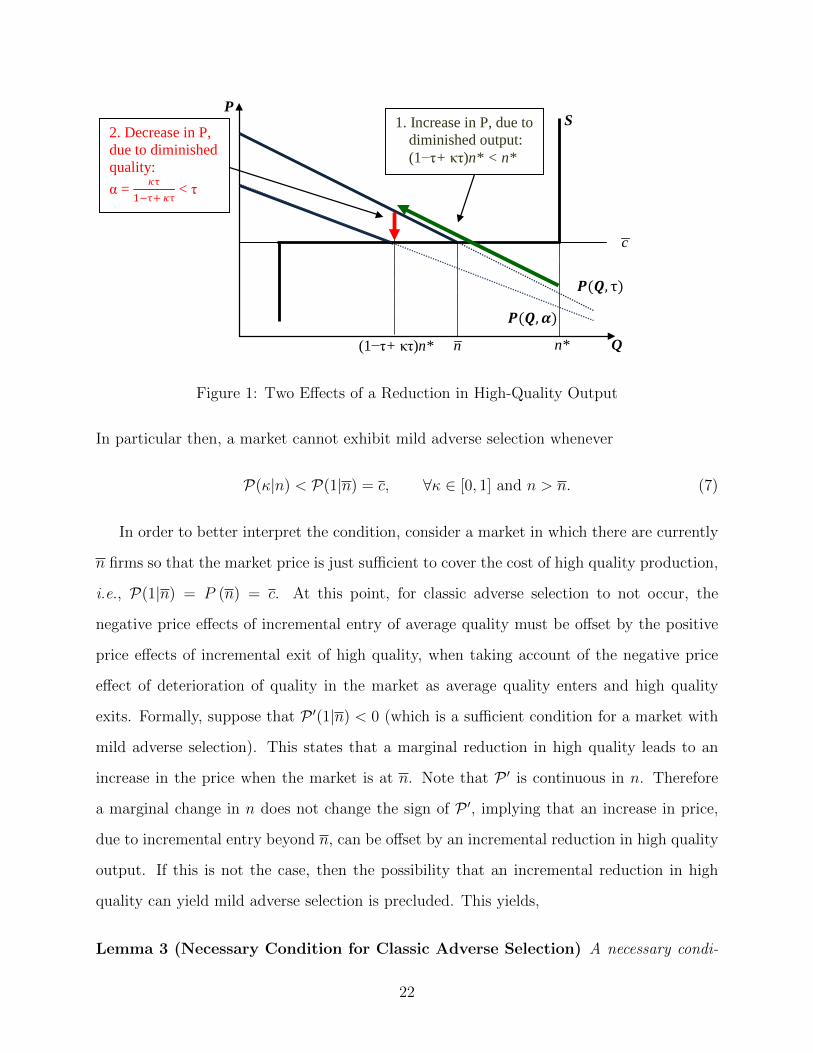
1. Increase in P, due to diminished output: (1−τ+ κτ)n* < n*

Q

P

c

S

n* n (1−τ+ κτ)n*

𝑷𝑷(𝑸𝑸,𝜶𝜶)

𝑷𝑷(𝑸𝑸, τ)

2. Decrease in P, due to diminished quality: α = 𝜅𝜅τ

1−τ+ 𝜅𝜅τ < τ

Figure 1: Two Effects of a Reduction in High-Quality Output

In particular then, a market cannot exhibit mild adverse selection whenever

P(κ|n) < P(1|n) = c, ∀κ ∈ [0, 1] and n > n. (7)

In order to better interpret the condition, consider a market in which there are currently

n firms so that the market price is just sufficient to cover the cost of high quality production,

i.e., P(1|n) = P (n) = c. At this point, for classic adverse selection to not occur, the

negative price effects of incremental entry of average quality must be offset by the positive

price effects of incremental exit of high quality, when taking account of the negative price

effect of deterioration of quality in the market as average quality enters and high quality

exits. Formally, suppose that P ′(1|n) < 0 (which is a sufficient condition for a market with

mild adverse selection). This states that a marginal reduction in high quality leads to an

increase in the price when the market is at n. Note that P ′ is continuous in n. Therefore

a marginal change in n does not change the sign of P ′, implying that an increase in price,

due to incremental entry beyond n, can be offset by an incremental reduction in high quality

output. If this is not the case, then the possibility that an incremental reduction in high

quality can yield mild adverse selection is precluded. This yields,

Lemma 3 (Necessary Condition for Classic Adverse Selection) A necessary condi-

22

tion for a market with classic adverse selection ( i.e., no mild adverse selection) is that

P ′(1|n) ≥ 0.

The condition given in Lemma 3 is not sufficient to assure that (7) holds, since mild

adverse selection need not be the result of a marginal adjustment process. In particular,

there are market constellations in which upon incremental entry beyond n mild adverse

selection emerges due to a (potentially large) positive measure of high quality firms ceasing

production. Indeed, in the example given in the introduction, if the cost of producing high

quality is given by 2.15, rather than 2.20, then upon entry of the eleventh firm in the market,

high quality cannot cover its cost even after the exit of one high-quality producer as the price

drops to 2.13. However, if two high quality producers simultaneously exit, the price increases

to 2.17, which is sufficient to cover high quality costs. That is, while a marginal reduction

in high quality output may not suffice to restore an equilibrium, a large reduction (falling

short of complete shut-down of high quality) may yield an equilibrium with mild adverse

selection.

We now consider conditions that render Lemma 3 sufficient for a market with classic

adverse selection.

Lemma 4 (Sufficient Condition for Classic Adverse Selection) A sufficient condition

for a market with classic adverse selection (given the condition in Lemma 3) is that

P ′′(κ|n) 6= 0,

i.e., P(κ) is either strictly concave or strictly convex in κ when evaluated at n.

Lemma 4 essentially imposes a regularity condition on the price adjustment process as

quantity and quality vary. The condition can be made weaker, since high quality being

driven entirely off the market only requires that once—for a fixed number of firms in the

market—the price reaches an extremum under variation in the quality make-up of supply,

then this extremum is not just local, but also global. For instance, either quasi-concavity or

quasi-convexity of P is also sufficient to guarantee the desired result.

23

We close this section with two final observations. First, while the primary argument

made is applied to conditions when there are n firms in the market, the proof of Lemma 4

establishes that mild adverse selection can be ruled out for measurable entry beyond n (i.e.,

a coordinated simultaneous entry of several firms). Second, it is straightforward to show that

Lemma 4 always holds when demand is not too convex (e.g., linear) and the price premium

function (viz., P − P ) is either decreasing or elastic whenever it is increasing.

3 Robustness

In this section we offer some results on the robustness of the insights by considering a

generalization and an extension. An obvious extension would be to allow for additional

periods of trading so that learning can take place. Indeed, this allows high quality firms to

reap profit in the future and therefore makes entry more attractive than in the base model.

But this is qualitatively equivalent to simply assuming a lower cost for the production of

high quality, and therefore such an extension results only in quantitative, but not qualitative

differences compared to the preceding analysis.

A less obvious question is what role discrete quality levels play in the base model. Hence,

we first consider a version of the model with a continuous distribution of types and derive

similar insights to those already established. A second question concerns the role that the

market structure has on the results. We address this by illustrating the main results by

sketching how in monopoly settings the same underlying effect of diminished entry (viz.

reduced capacity) also occurs when the firm invests in order to produce a good of uncertain

quality.

3.1 Continuous Distribution of Quality

Though we considered discrete distributions of quality thus far, the results do not crucially

depend on discreteness. Specifically, suppose that quality, which is indexed by s, is dis-

tributed ex ante according to the strictly increasing and twice differentiable distribution

24

function F (s) on [s, s]. The cost associated with producing a unit of the good with qual-

ity index s is given by the strictly increasing twice differentiable function C(s). Given the

Pareto selection criterion in conjunction with the law of one price, if it is profitable for a

firm of quality index σ ∈ [s, s] to produce, it is also profitable for all firms with quality

index s ≤ σ to produce. All other assumptions on firms remain the same. In particular, we

consider a continuum of firms who each observe an independent draw from the distribution

of quality parameters F (s) upon entry. Consequently there is no aggregate uncertainty and

the distribution of quality among the firms in the market is also characterized by F (s).19

Demand for quality s is given by p(Q, s), which is twice differentiable and decreasing

in market output Q and increasing in quality s. Define demand for the case that σ is the

highest level of quality on offer by P (Q, σ) :=∫ σs

p(Q,s)F (σ)

dF (s) and it follows that P (Q, σ)

is also twice differentiable, decreasing in Q, and increasing in σ. Assume that the lowest

quality alone cannot support efficient market transactions, i.e., P (0, s) ≤ C (s); whereas

there is potential for trade given the ex ante average quality, i.e., P (0, s) > C (s). Assuming

limQ→∞ P (Q, σ) = 0 yields that n is implied by P (n, s) = C(s).

It readily follows that the analogue to Proposition 1 holds with ι = C (s) − Ec, where

Ec :=∫ ssC(y)dF (y) is the expected cost of a firm under the prior. For this case n∗ is then

implied by P (n∗, s) = ι+ Ec with ι ≥ ι.

In order to distinguish the cases of classic adverse selection from mild adverse selection

define similarly to (6),

E(σ|n) := P (nF (σ), σ)− C(σ). (8)

That is, E(σ|n) is the equilibrium market profit (i.e., earnings) of the marginal producer

with quality index σ, given that n firms are in the market.20

We define classic adverse selection in this context as a case where a marginal deterioration

of quality leads to a market collapse, i.e., a discrete drop in average quality and market price

19An implication of the continuous distribution of quality is that in contrast to the previous section theequilibrium entails pure strategies.

20Because in the two-type case there is only one cost-type (the high cost firm) who makes the marginaldecision on whether to produce, (6) does not contain an expression for costs, whereas here each firm hasdistinct costs which must be considered explicitly.

25

so that no firms continue to produce. In contrast, mild adverse selection entails marginal

exit of high quality in such a way that prices adjust smoothly to the altered conditions in

the composition of supply. Hence, analogous to (7), the condition that characterizes markets

with classic adverse selection is given by

E(σ|n) < E(s|n) = 0, ∀σ ∈ [s, s] and n > n.

The necessary and sufficient conditions for a market to exhibit classic adverse selection are

derived analogous to Lemmata 3 and 4, yielding

E ′(s|n) ≥ 0,

E ′′(σ|n) 6= 0.

Intuitively speaking the necessary condition assures that if entry beyond n takes place

so that the price decreases due to the increased supply, profit of firms at the upper end of

the quality support decrease, which implies that a positive measure of high quality firms

must cease production. The sufficient condition then guarantees that not only do a positive

measure of firms near the upper end of the quality support exit, but so do in fact firms of

all quality types.

Given these conditions, the results of positive profits and no adverse selection in the

market (Proposition 1) and positive profits with mild adverse selection (Proposition 2) carry

over with only minor qualifications to the current setting as illustrated in the following two

examples.

Example 1 (Positive Profits and No Adverse Selection) Let quality be distributed uni-

formly on the unit interval, i.e., F (s) = s on [0, 1] and let costs be given by C(s) =√s/3.

Demand for given quality is p(Q, s) = s(1−Q), so P (Q, σ) =∫ σ

0s(1−Q)

σds = (σ/2)(1−Q).

Given these parameters, E(σ|n) = (σ/2)(1−nσ)−√σ/3 and E ′(σ|n) = 1/2−nσ−1/6

√σ. The

full production threshold n is implied by P (n, 1) = C(1), i.e., (1/2)(1 − n) = 1/3, so n = 1/3.

Thus, E ′(σ = 1|n = 1/3) = 1/2 − 1/3 − 1/6 = 0, so the necessary condition for classic adverse

26

selection is met. Note that when entry is at n = 1/3 average market profits are given by

P (n, s)−∫ ssC(s)dF (s) = P (1/3, 1)−

∫ 1

0(√s/3)ds = (1/2) (1− 1/3)− 2/9 = 1/9. Hence, ι = 1/9.

Now consider n > n = 1/3 and note that the highest quality producer’s market profit must

be zero. From (8) we have

E(σ|n > n) = P (nF (σ), σ)− C(σ) =σ

2(1− nσ)−

√σ

3= 0. (9)

However, for all n > n = 1/3, (9) does not have a non-negative root in σ so there exists no

market equilibrium with production for n > n and therefore ι = 0, n∗ = n = 1/3 and in the

entry equilibrium firms make an average profit of 1/9− ι > 0.

Example 2 (Positive Profits with Mild Adverse Selection) Consider Example 1, now

with costs given by C(s) =√s/4. Then n = 1/2, since (1/2)(1 − n) = 1/4; and E ′(σ = 1|n =

1/2) = 1/2 − 1/2 − 1/8 = −1/8 < 0, so the necessary condition for classic adverse selection is

violated ( i.e., the sufficient condition for mild adverse selection is met).

Note that when n = 1/2 firms enter, average market profits are P (1/2, 1) −∫ 1

0(√s/4)ds =

(1/2) (1− 1/2)− 1/6 = 1/12, so ι = 1/12.

Now, analogous to (9), the equilibrium condition for the highest level of quality for entry

beyond n = 1/2 is given by

E(σ|n > n) =σ

2(1− nσ)−

√σ

4= 0. (10)

This equation does have a root in σ provided that n ≤ 16/27, but not for entry beyond that,

so n′ = 16/27. At n′ (10) reveals that σ = 9/16. A firm’s expected market profit (after entry,

but before quality and costs are realized) at this point is given by F (σ)E(σ|n′) = 9/256. So for

ι ∈ [0, 9/256), n∗ = 16/27 and equilibrium profit is 9/256− ι > 0.

The main distinction between Proposition 2 for the discrete case and Example 2 for a con-

tinuous distribution of quality concerns firms’ profits under mild adverse selection. In par-

ticular, where in Proposition 2 firms retain positive profit for any entry cost between ι′ and

ι, this is not the case in Example 2. Specifically, the entry equilibrium configuration for

27

ι ∈ [9/256, 1/12 = ι] entails zero expected profit as firms enter beyond n = 1/2 and quality

gradually adjusts with the implied price decline. However, such gradual adjustment is not

possible beyond n∗ = 16/27 at which point a positive profit equilibrium emerges when entry

costs are below 9/256.

3.2 Monopolistic Markets

Having shown that limited entry and above normal profit can occur even under costless

entry in Walrasian markets due to latent adverse selection, we briefly consider the case of

monopolistic markets.21 As the monopoly market implies restricted entry, it is clear that

profits are expected to occur in equilibrium and therefore the point of this section is to

demonstrate that latent adverse selection nonetheless affects the market equilibrium. In

particular, the potential for adverse selection still leads to “limited entry,” but now in terms

of a reduced capacity choice by the monopolistic firm. Coupled with the result is, similar to

the other models, that the market equilibrium exhibits no adverse selection.

Formally, we suppose that the firm incurs an investment outlay of ι in order to obtain an

observable production capacity which, for purposes of congruence with the base model, we

denote by n. After the capacity decision, the firm observes the quality of its product as being

high with probability τ or otherwise low. In order to not distract from the point at hand,

we preclude signalling equilibrium configurations by assuming that low quality alone cannot

sustain sales, which implies that a low quality-producer will always mimic the strategy of the

high-quality producer, thus, eliminating any separating equilibrium. Once the firm knows

its quality and costs, it chooses a price and then produces output Q ≤ n.

Example 3 (Reduced Capacity Choice) Suppose τ = 2/3; demand for known high qual-

ity is given by P = 6(1−0.05Q), whereas there is no demand for low quality. Hence demand

for average quality is P = 4(1− 0.05Q). Unit cost of high quality is c = 3 and c = 0. Con-

21Since Akerlof’s seminal paper much of the theoretical literature has actually departed from his anal-ysis by focusing on monopoly settings (and thereby precluding entry). See, e.g., Milgrom and Roberts(1986), Daughety and Reinganum (1995), but also the more recent work by Hendel and Lizzeri (2002) andBelleflamme and Peitz (2009).

28

sumers (rationally) anticipate that a high quality producer would leave capacity unused, if

the price is below c, since this price is below the unit cost of production. However, above this

price, as either type would in fact sell (and the low quality producer would sell whatever the

high quality producer sells at these prices), demand follows the demand for expected quality.

In sum

P =

4(1− 0.05Q) if Q < 5

0 if Q ≥ 5.

Thus, the firm will only be able to sell when facing demand of P = 4(1− 0.05Q). If the firm

has high costs, it produces Q∗ = 2.5, which is also produced if the firm has low cost in order

to mimic the high cost firm. Hence n∗ = 2.5.

In contrast, if the firm were to be known to produce high quality its output is 5 and it is

0 if it is known to produce low quality, yielding an average output of nFI := (2/3)5 + (1/3)0 =

10/3 > 2.5 = n∗. And optimal output under average quality produced at average costs is

nAvge := 5 > 2.5 = n∗. Thus, one obtains reduced capacity compared to either benchmark

with ι = 0.

Since positive profit naturally occurs in the monopolistic setting, this cannot be used to

empirically detect the impact of the potential of adverse selection on the market. Notice,

however, that if data can be obtained on the expectation of marginal costs, then if this

average is below marginal revenue this is an empirical indication of lower than expected

capacity, due to latent adverse selection.

4 Conclusion

In this paper we examine how markets with the salient features of adverse selection are

affected when the heretofore exogenous number of firms is made endogenous. Firms enter

through a fixed investment after which nature chooses the quality of the firm’s product that

is unobservable to consumers. It is found that the potential for adverse selection—low quality

producers driving out high quality ones—affects the market even though adverse selection

29

does not arise in equilibrium. Indeed, such latent adverse selection leads to entry equilibrium

configurations with positive profits, even under the assumption of costless entry.

Unobserved adverse selection in conjunction with positive profits is the result of the

interaction of two classic mechanisms. First, as demand slopes downward less entry results

in higher prices. Second, average quality is increasing in market prices so that if the market

price is high enough, then high quality producers are willing to produce. Hence, zero profits

may no longer define the entry equilibrium. Instead the entry equilibrium is defined by the

greatest level of entry under which adverse selection does not occur ex post. That is, latent

adverse selection is an entry barrier, and whenever it defines the entry equilibrium then

equilibrium profits are positive even under costless entry.

While the primary derivation is performed for discrete quality distributions in Walrasian

markets, we show that the insights—viz. limited entry, positive equilibrium profits that

exceed entry costs, and the absence of observed adverse selection—hold for generalized (con-

tinuous) distributions and the result of latent adverse selection as an entry barrier carries

over to the monopoly setting in the form of reduced capacity.

The theoretical analysis provides some additional insights. First, the role of downward

sloping demand suggests it may play an important role in models of endogenous quality that

heretofore have used unit demand—indeed, in our setting downward sloping demand gives

rise to a form of “mild” adverse selection in which only some high quality producers exit the

market. Secondly, it is found that the equilibrium outcome of limited entry prevents welfare

losses stemming from adverse selection so that overall welfare is greater despite profits not

dissipating. Nevertheless, welfare can be raised further through a revenue-neutral policy of

an investment tax and a production subsidy. The revenue neutrality implies that even an

incorrectly set tax and subsidy raises welfare.

As the model yields equilibrium configurations in which adverse selection is not an equi-

librium phenomenon the insights may contribute to our understanding of why empirical

evidence of adverse selection in markets is often lacking. In particular, the findings suggest

that in industries with high entry costs one would not find either direct or indirect empirical

30

evidence of adverse selection, even though the market exhibits the characteristics for adverse

selection. In cases of lower entry costs, indirect empirical evidence for latent adverse selec-

tion can be found in the absence of actual adverse selection coupled with positive profits

that are not competed away. These observations taken together imply a negative correla-

tion between entry costs and profitability, which may be a contributing explanation to the

somewhat counter-intuitive empirical finding that entry is slow to react to high profits.22

The insights and conclusions from the model may be particularly applicable in industries

with frequent innovations, as in these instances the results of R&D are frequently not known

with certainty ex ante and product life-cycles may be sufficiently short to result in frequent

new ‘investment/entry’ even of previously existing firms (e.g., consumer electronics). Similar

situations may arise when output is tied to heterogenous inputs (e.g., in order to diversify

bottleneck risks many manufacturers multi-source their procurement which can result in non-

uniform quality across suppliers and subsequent variations in the quality of the final product);

and in high-end agricultural (e.g., viniculture, where quality is subject to exogenous shocks

such as weather) and animal breeding, which entails uncertain and hard-to-verify outcomes

(e.g., horse-breeding, where lineage does not guarantee winnings).

In addition to these applications, alternative interpretations of the model yield additional

insight. One such possibility is to reinterpret n so that rather than considering de novo entry,

one examines existing firms’ output decisions. For instance, a mortgage lender—who can

only gauge the specific quality of a loan after it has originated—can decide to keep it, or sell

it in the secondary market, where—as has become abundantly clear in the last years—quality

has been proven hard to verify. Similarly car dealers must decide whether to keep trade-ins

in their inventory or whether to sell them off to other markets.

Finally, while the exposition of the paper is in keeping with Akerlof’s original notion of

adverse selection, the analysis is of course isomorphic for markets with experience or credence

goods, including instances in which products are differentiated by production or distribution

characteristics (e.g., ‘sustainable,’ ‘fair trade’ and other attributes) that are unobservable

22See, e.g., Geroski’s widely cited review of the empirical literature on entry (Geroski, 1995, p. 427).

31

and hard to verify.

Appendix of Proofs

Proof of Proposition 1. Suppose first that no adverse selection occurs in the market.

Then demand is given by P (Q,α) = P (n, τ). Since P (n, τ) is decreasing in n, entry ceases

once the price is just sufficient to cover the expected production cost Ec and the entry cost

ι, i.e., equilibrium entry is defined by P (n∗, τ) = ι+Ec, proving the first statement. At this

price, expected market profits are Eπ = P (n∗, τ)−Ec = ι, proving the second statement. In

order to confirm our initial supposition it must be that the price is sufficiently high to cover

the costs of the high quality producer. That is, P (n∗, τ) = ι + Ec = ι + τc + (1 − τ)c ≥ c.

Let ι = (1− τ)(c− c). �

Proof of Proposition 1. An implication of Lemma 1 is that since ι < ι entry assuredly

takes place at least till n. Beyond that, take the proposed entry equilibrium as given and

consider the marginal firm at n∗. Since n∗ = n, incremental entry triggers adverse selection.

Because the market then exhibits classic adverse selection, all high quality producers shut

down. Thus, the only possibility of obtaining positive market profit for the marginal firm

is if it is a low quality (and hence low cost) producer. Upon entry, if all low quality firms

produce, the resulting market price is P ((1− τ)n, 0). If P ((1− τ)n, 0) ≤ c, then firms

make no profit so that incremental entry beyond n∗ = n does not pay off, even under the

assumption of costless entry. Hence, let ι = 0 and all three statements of the proposition

follow readily.

Suppose instead that P ((1− τ)n, 0) > c. Then, if the marginal firm enters and is a low

quality producer, its profit is P ((1− τ)n, 0)−c. Hence, the marginal firm’s expected market

profit prior to but conditioned on incremental entry is given by (1− τ) (P ((1− τ)n, 0)− c).

Let ι = (1− τ) (P ((1− τ)n, 0)− c) and it is clear that entry beyond n does not take place.

Note finally that since P ((1− τ)n, 0) < P (0, 0) < c, it follows that ι < ι. This es-

tablishes that equilibrium profits are positive, since Eπ(n∗) = Eπ(n) = P (n, τ) − Ec =

32

c− (τc+ (1− τ)c) = (1− τ)(c− c) = ι > ι. �

Proof of Lemma 2. First, by definition of n there exists a full-production equilibrium with

no adverse selection for n ≤ n. Thus, given the Pareto equilibrium selection criterion, mild

adverse selection cannot occur for any n ≤ n, so we require that n > n (which precludes

κ = 1).

Second, note that P < c cannot be an equilibrium since it entails negative market profits

for high quality producers, which are avoided by shutting down (implying κ = 0); and P > c

cannot be an equilibrium as an idle high-quality producer increases profit by producing and

selling a unit of the good. Hence, for an equilibrium with mild adverse selection to occur, it

must be that P = c.

At this price all low quality firms produce, yielding output of (1− τ)n. If a fraction κ of

the τn high quality firms produce, market output is thus (1−τ +κτ)n and the proportion of

high quality is κτ1−τ+κτ

. Therefore the existence of a κ such that (5) holds for some n > n is

a necessary and sufficient condition for the market to have an equilibrium with mild adverse

selection. �

Proof of Proposition 2. As in the proof to Proposition 1, note that an implication of

Lemma 1 is that since ι < ι entry assuredly takes place at least till n. However, unlike in

the proof of Proposition 1, from Lemma 2, given mild adverse selection there exists n > n

such that the expected market price is P = c; and, therefore, entry continues beyond n;

confirming the first claim in the proposition.

Now define n′ as the largest number of firms such that mild adverse selection can be

sustained, i.e., P (n′) = c and P (n) < c,∀n > n′. Then the remainder of the proof fol-

lows the proof of Proposition 1 mutatis mutandis with n′ replacing n. In particular, if

P ((1− τ)n′, 0) ≤ c, let ι′ = 0; and if P ((1− τ)n′, 0) > c, let ι′ = (1−τ) (P ((1− τ)n′, 0)− c).

�

Proof of Proposition 3. Note first that market welfare is increasing in n for n ≤ n.

Consider now welfare for n ≥ n and denote by κ the portion of high quality firms who

produce in the market so that κ = 0 in markets with classic adverse selection and κ ∈ (0, 1)

33

in markets with mild adverse selection. Market output is thus given by Q = (1 − τ + κτ)n

and the proportion of high quality in the market is given by α = κτ1−τ+κτ

< τ .

Welfare at n is given by

W (n) = CS(n) + n× Eπ(n) =

∫ n

0

[τP + (1− τ)P − c

]dQ+

∫ n

0

(1− τ)(c− c)dQ

=

∫ (1−α)n

0

[τP + (1− τ)P − c

]dQ+

∫ n

(1−α)n

[τP + (1− τ)P − c

]dQ

+

∫ (1−α)n

0

(c− c)dQ+

∫ (1−τ)n

(1−α)n

(c− c)dQ.

The second and fourth integral are both positive, let their sum be denoted by A; and the

first and third can be combined to yield

W (n) =

∫ (1−α)n

0

[τP + (1− τ)P − c

]dQ+ A.

When replacing τ with α in the integral, the integral itself is the market welfare under

incremental entry beyond n. However, as τ > α, P > P > 0 and A > 0, there is a discrete

fall in welfare upon entry beyond n. Note lastly that for entry beyond that welfare decreases

as average profit weakly decreases and output and average quality also decrease; with another

discrete fall in welfare at n′ in the case of markets with mild adverse selection. �

Proof of Lemma 4. If P(κ|n) is convex, then it lies below any of its secant lines. Consider

the secant line constructed from the points κ = 0 and κ = 1, i.e., S(κ) := P(0|n) +

[P(1|n)− P(0|n)]κ; or S(κ) = (1−κ)P ((1− τ)n, 0)+κc, since P(0|n) = P ((1− τ)n, 0) and

P(1|n) = c. Notice that P ((1− τ)n, 0) < P (0, 0), since P is decreasing in its first argument.

Since P (0, 0) < c, it follows that P(κ|n) < S(κ) < (1− κ)P (0, 0) + κc < c, ∀κ ∈ (0, 1).

Now suppose that P(κ|n) is concave. Then the function lies below any of its tangent lines.

Since P ′(1|n) > 0, it therefore follows that P(κ|n) < P(1|n) = c, ∀κ < 1. Hence, regardless

of whether P(κ|n) is concave or convex, P(κ|n) < c, ∀κ ∈ (0, 1) so that incremental entry

beyond n does not result in mild adverse selection.

Note finally that ddnP =

((1− α)P ′ + αP

′)

(1− τ + τκ) < 0 so that P(κ|n) < c, ∀n >

n, violating Lemma 2 and, thus, ruling out mild adverse selection for any n ≥ n. �

34

References

[1] Ackerberg, D., 2003, Advertising, Learning, and Consumer Choice in Experienced Good

Markets: An Empirical Examination, International Economic Review, 44(3), 1007–1040.

[2] Akerlof, G., 1970, The Market for Lemons: Qualitative Uncertainty and the Market

Mechanism, Quarterly Journal of Economics, 84, 488–500.

[3] Ashenfelter, O., 2008, Predicting the Quality and Prices of Bordeaux Wine, Economic

Journal, 118, F174–F184.

[4] Belleflamme, P. and M. Peitz, 2009, Asymmetric Information and Overinvestment in

Quality, CESifo Working Paper Series No. 2619.

[5] Bennardo, A. and P.-A. Chiappori, 2003, Bertrand and Walras Equilibria under Moral

Hazard, Journal of Political Economy, 111(4), 785–817.

[6] Bond, E., 1982, A Direct Test of the ’Lemons’ Model: The Market for Used Pickup

Trucks, American Economic Review, 71(3), 836–840.

[7] Caves, R.E. and D.P. Greene, 1996, Brands’ quality levels, prices, and advertising out-

lays: empirical evidence on signals and information costs, International Journal of In-

dustrial Organization, 14, 29–52.

[8] Chezum, B. and B. Wimmer, 1997, Roses or Lemons: Adverse Selection in the Market

for Thoroughbred Yearlings, Review of Economics and Statistics, 79(3), 521–526.

[9] Chu, S., 2011, Adverse or maybe not-so-adverse Selection in the CMBS Market, mimeo,

Federal Reserve Board.

[10] Creane, A., 1994, Adverse Selection, Moral Hazard and Entry, CERGE-EI Discussion

Paper No. 42.

[11] Dana, J., 2001, Competition in Price and Availability when Availability is Unobservable,

RAND Journal of Economics, 32(3), 497–513.

35

[12] Daughety, A. and J. Reinganum, 1995, Product Safety: Liability, R&D, and Signaling,

American Economic Review, 85(5), 1187–1206.

[13] Daughety, A. and J. Reinganum, 2005, Secrecy and Safety, American Economic Review,

95(4), 1074–1091.

[14] Dell’Ariccia, G., E. Friedman, and R. Marquez, 1999, Adverse Selection as a Barrier to

Entry in the Banking Industry, RAND Journal of Economics, 30(3), 515–534.

[15] Deneckere, R., H.P. Marvel, and J. Peck, 1997, Demand Uncertainty and Price Main-

tenance: Markdowns as Destructive Competition, American Economic Review, 87(4),

619–641.

[16] Dionne, G., P. St-Amour, and D. Vencatachellum, 2009, Asymmetric Information and

Adverse Selection in Mauritian Slave Auctions, Review of Economic Studies, 76, 1269–

1295.

[17] Etro, F., 2006, Aggressive Leaders, RAND Journal of Economics, 37(1), 146–154.

[18] Etro, F., 2011, Endogenous Market Structures and Contract Theory: Delegation,

Principal-Agent Contracts, Screening, Franchising and Tying , European Economic Re-

view, 55(4), 463–479.

[19] Farrell, J., 1986, Moral Hazard as an Entry Barrier, RAND Journal of Economics,

17(3), 440–449.

[20] Financial Times Information, 2000, Acer and Hitachi Expand Joint Production of DVD

Players, December 19.

[21] Genesove, D., 1993, Adverse Selection in the Wholesale Used Car Market, Journal of

Political Economy, 101(4), 644–65.

[22] Geroski, P.A., 1995, What do we know about entry? International Journal of Industrial

Organization, 12, 421–440.

36

[23] Gerstner, E., 1985, Do Higher Prices Signal Higher Quality? Journal of Marketing

Research, 22(2), 209-215.

[24] Ghosal, V., and P. Loungani, 2000, The Differential Impact of Uncertainty on Invest-

ment in Small and Large Businesses, Review of Economics and Statistics, 82(2), 338–349.

[25] Guiso, L. and G. Parigi, 1999, Investment and Demand Uncertainty, Quarterly Journal

of Economics, 185–227.

[26] Heimoff, S., 2009, The Rise of the California Negociants, Wine Enthusiast, 21(5), 44–48.

[27] Hendel, I. and A. Lizzeri, 2002, The Role of Leasing under Adverse Selection, Journal

of Political Economy, 110(1), 113–143.

[28] Hendel, I., A. Lizzeri, and M. Siniscalchi, 2005, Efficient sorting in a dynamic adverse-

selection model, Review of Economic Studies, 72(2), 467–497.

[29] Hjorth-Andersen, C., 1991, Quality Indicators in Theory and in Fact, European Eco-

nomic Review, 38(5), 1491–1505.

[30] Hopenhayn, H.A., 1992, Entry, Exit, and Firm Dynamics in Long Run Equilibrium,

Econometrica, 60(5), 1127–1150.

[31] Horner, J,. and N. Vielle, 2009, Public vs. Private Offers in the Market for Lemons,

Econometrica, 77(1), 29–60.

[32] Hovenkamp, H., 1989, The Antitrust Movement and the Rise of Industrial Organization,

Texas Law Review, 68(1), 105–67.

[33] Jenks, J.W., 1888, The Michigan Salt Association, Political Science Quarterly, 3(1),

78–98.

[34] Jenks, J.W., 1889, The Development of the Whiskey Trust, Political Science Quarterly,

4(2), 296–319.

37

[35] Johnson, J.P. and M. Waldman, 2003, Leasing, Lemons, and Buybacks, RAND Journal

of Economics, 34(2), 247–265.

[36] Jones, E., 1914, The Anthracite Coal Combination in the United States, Harvard Eco-

nomic Studies No. 11, Harvard University Press.

[37] Jones, E., 1920, Is Competition in Industry Ruinous, Quarterly Journal of Economics,

34(3), 473–519.

[38] Jovanovic, B., 1982, Selection and the Evolution of Industry, Econometrica, 50(3), 649–

670.

[39] Klein, B. and K. Leffler, 1981, The Role of Market Forces in Assuring Contractual

Performance Journal of Political Economy, 89, 615–641.

[40] Lacko, J.M., 1986, Product Quality and Information in the Used Car Market, Bureau

of Economics Staff Report, FTC.

[41] Lonsford, M., 2002a, Wine: Burgundy’s Burden, Houston Chronicle, 19 February 2002.

[42] Lonsford, M., 2002b, Wine: Sonoma roots, Houston Chronicle, 7 May 2002.

[43] Milgrom, P. and J. Roberts, 1986, Price and Advertising Signals of Product Quality,

Journal of Political Economy, 94(4), 796–821.

[44] OECD, 2008, Roundtable on Competition in the Construction Industry, Director for

Financial and Enterprise Affairs, Competition Committee, Discussion Paper.

[45] Riley, J.G., 2002, Silver Signals: Twenty-Five Years of Screening and Signaling, Journal

of Economic Literature, 39, 432–478.

[46] Rose, C., 1993, Equilibrium and Adverse Selection, RAND Journal of Economics, 24(4),

559–569.

[47] Schmalensee, R., 1982, Product Differentiation Advantages of Pioneering Brands, Amer-

ican Economic Review, 72, 349–365.

38

[48] Sultan, A., 2008, Lemons hypothesis reconsidered: An empirical analysis, Economics

Letters, 99, 541–544.

[49] Wiener, J.L., 1985, Are Warranties Accurate Signals of Product Reliability? Journal of

Consumer Research, 12(2), 245-250.

[50] Wilson, C.A., 1980, The Nature of Equilibrium in Markets with Adverse Selection, Bell

Journal, 11(1), 108–130.

39