ENDOGENEITY IN THE CAPM - Trade2Win€¦ · ENDOGENEITY IN THE CAPM Can OLS regression yield...

EC331 Research in Applied Economics 0 5 0 5 1 8 1

ENDOGENEITY IN THE

CAPM

Can OLS regression yield unbiased beta estimates when

using the CAPM to estimate the cost of equity for a FTSE

100 firm?

Department of Economics,

University of Warwick

April 2008

5986 Words1 2

Abstract

This study uses data from the FTSE 100 to look at the extent to which the market

return is an endogenous variable when using the CAPM and the problems that this

causes in beta estimation. The ordinary least squares method of beta estimation is

compared to an unbiased “instrumental variable” estimate and the bias is then tested

for significance using a form of the Hausman test. A simple model for the bias is then

formed, that takes into account changing market conditions through shifts in the

covariance matrix. The implications of the endogeneity on beta stability, a major area

of previous research, are then investigated. This paper finds that endogeneity is a

significant problem in the FTSE 100 and that this may have serious implications for

studies of beta stability. By using data from a market in which there is no lack of

liquidity, the distinction between thin-trading bias and endogeneity bias is made

clearer than it has been in previous literature.

1 Main body-text only, excludes abstract, contents, tables, references, appendices and boxed text.

2 I would like to thank Professor Valentina Corradi for her guidance and support throughout this work;

her advice has been pivotal at every stage of the study. I would also like to thank Professor

Anthony Neuberger for offering his specialist knowledge in beta estimation. All errors and omissions

are the sole responsibility of the author.

EC331 ENDOGENEITY IN THE CAPM 0 5 0 5 1 8 1

2

CONTENTS

• I: Introduction

• II: Theory and Literature review II.1: A brief introduction to the CAPM II.2: Beta estimation II.3: Sources of error in beta estimation

� Endogeneity bias

� Beta instability

� Thin trading bias

• III: Empirical Strategy III.1: Selecting the data

III.2: Constructing the index

III.3: Determining the size of the bias

III.4: Testing the significance of the bias

III.5: Modelling the size of the bias

III.6: Effect of the bias on beta stability

• IV: Data and Results IV.1: Preliminary data analysis

IV.2: Summary statistics

IV.3: Hausman test results

IV.4: Modelling the size of the bias

IV.5: Effect of bias on beta stability

• V: Conclusions and Extensions V.1: Conclusions

V.2: Limitations and Extensions

• References

• Appendices A.1: Description of variables

A.2: Regression outputs

A.3: Beta instability results

3

4

5

6

11

11

12

14

14

15

16

20

22

23

27

31

32

33

35

37

40


3

I: INTRODUCTION

The Capital Asset Pricing Model (CAPM) is perhaps the most celebrated

development in modern financial theory, with its findings concerning the risk-return

trade-off being the foundations upon which four decades of financial theory has been

based.

Fama and French (1992) found significant evidence that the CAPM had little

predictive ability and that the securities market line (SML), relating beta to expected

return, was flat. However, as emphasised by Black (1998), if the SML is flat, it

becomes optimal to actively seek out the portfolio with the lowest possible beta. This

leads us to the conclusion that even if the CAPM is dead, beta is still very much alive!

Whatever the relative merits of the CAPM, it is clear that accurate beta estimation is

still a highly important area of research. Inaccurate beta estimates can lead investors

to make sub-optimal asset allocation decisions or cause a firm to miscalculate their

cost of equity and pursue unprofitable ventures.

The literature has focused on two major sources of error in beta estimation: thin-

trading bias and beta stability over time. However, there is a third source of error in

beta estimation that may be at least as significant as the two aforementioned sources

and has not received nearly as much attention. This is the bias caused by the

endogeneity of market returns.

The standard method of beta estimation is to use the ordinary least squares method

to regress the excess returns to the asset on the excess returns to the market.

However, in the CAPM “the market” should be representative of “all wealth”,

something that is almost impossible to measure.3 Instead, market indices are used as

a proxy. However, when looking at shares, this is often the index of which they are a

constituent. The ordinary least squares regression then involves regressing the

3 See (Roll 1976), commonly known as “The Roll Critique” for a full explanation of the inadequacy of

using a market index as a proxy for “all individual assets”.


4

returns to the share on the returns to the index, which are, to some extent, decided by

the returns to the share! Clearly, this leads to the market returns being endogenous

and beta estimates to be biased.

It has been shown by Woo, Cheung and Yan-Ki Ho (1994) that this represents a

serious problem on emerging Asian stock markets (EASMs). Their discussion of the

causes of this bias is vague in differentiating between endogeneity caused by thin-

trading (a lack of liquidity) and the endogeneity caused by high index weightings. By

adapting their methods and applying them to the shares of one of the most actively

traded markets in the world, the FTSE 100, this paper provides a number of further

insights into the problem of endogeneity bias in beta estimation as well as its effects

on attempts to investigate beta stability over time.

II: THEORY & LITERATURE REVIEW

II.1: A BRIEF INTRODUCTION TO THE CAPM

The CAPM4 is used to determine a theoretically appropriate required rate of return

for an asset. It is the simplest version of a family of equations that express expected

returns as a linear function of one or more macro-economic variables.

The CAPM model

E(ra) – rf = βa [E(rm) – rf]

Where ra is the return on the asset, rf is the risk free rate of return, E(.) denotes an

expected value and βa measures the sensitivity of the asset’s returns to the returns of

the market.

4 The CAPM is often credited solely to Sharpe (1964). This ignores, however, the important

contributions of Treynor (1961), Lintner (1965) and Mossin (1966). Sharpe was the only one of the

four to receive a Nobel Prize for the contribution.


5

It assumes that the asset is to be added to an already well-diversified portfolio and

therefore that only market risk should be rewarded with higher returns. Having

made some broad assumptions, the CAPM goes on to reach some rather startling

conclusions, namely that no possible portfolio of assets can be expected to outperform

the market portfolio.

The equation has many practical uses for both firms and investors. Firms can use the

CAPM as a tool for estimating their cost of equity, the amount that new shareholders

would demand for taking on the risk of the firm. Investors can use the CAPM to

determine the rate of return that they can expect from an asset. This will be

particularly useful to them if they are adding the asset to an already well diversified

portfolio as they will have no reason to be concerned with any kind of idiosyncratic

risk, which is ignored by the CAPM.

II.2: BETA ESTIMATION

The most common method of beta estimation is to estimate the following equation

using an ordinary least squares (OLS) regression:

Estimating beta using OLS

[rJ t – rf t ] = βJ [rm t – rf t] + εJ

Given that this method is to be used, there are still two important decisions to be

made; the frequency of returns and the length of the time period to be used.

Daves, Ehrhardt and Kunkel (2000) emphasise the trade-off between the two issues;

the use of more observations in the sample has the advantage of a reduced standard

error, but if it involves a longer estimation period then it has the disadvantage of

being more likely that beta has changed during the period. They use a large data-set


6

to attempt to reach a definitive answer to the two issues.

With regard to the frequency of returns, they find that daily returns provide the

optimal results for all liquid shares5 due to meaningful reductions in standard error.

The caveat that the shares must be liquid for daily data to be optimal is in line with

the findings of Cohen, Hawawini, Maier, Schwartz & Whitcomb (1983), who were

the first to examine the effect of micro-structural issues on the appropriate return

interval to use. They stress that the most important of these issues is the price

adjustment delay and where this is significant, daily data can lead to biased results.

They also suggest that where these delays are short or non-existent, shorter return

intervals were appropriate.

With regard to the optimum estimation period, Daves, Ehrhardt and Kunkel (2000)

go on to find that a period of three years is optimal, as it captures the majority of the

reduction in the standard error of the estimate, as well as minimising the risk that

beta has changed during the time period. This stands in contrast to much of the

earlier literature6, such as that contributed by Gonedes (1973) and Baesel (1974), that

recommend periods of seven and nine years respectively.

II.3: SOURCES OF ERROR IN BETA ESTIMATION

There are three main sources of error in beta estimation. These are beta instability

during the time period, thin trading bias caused by large differences in liquidity

between shares and the bias caused by the endogeneity of market returns. When two

or more of these are affecting estimates simultaneously, it can be hard to differentiate

5 They recognise that the findings may not apply directly to less liquid shares for which micro-

structural issues such as stale prices may exist.

6 We cannot take this as strong evidence that there has been a dramatic change in the level of beta

stability in the last few decades. This is because it could easily be a result of the switch to using daily

data; when using weekly data, nine years provides a substantial advantage to three years but when

using daily data, the advantage is smaller.


7

between them. This study is investigating the effects of only one of these sources of

error, endogeneity, but it is crucial to understand the nature of the other two in order

to properly separate them.

Endogeneity of market returns

This paper was largely influenced by the work of Woo, Cheung and Yan-Ki Ho

(1994). They show that beta estimates in “small stock markets” are biased upwards

due to the endogeneity of market returns. They do this by applying the Hausman

(1978) specification test for endogeneity to the returns of stocks in two small stock

markets, Hong Kong and Thailand.

They find that every share that they examined has significant evidence of

endogeneity according to the Hausman test and that comparing the OLS estimates to

unbiased IV estimates results in biases of up to 7%.

There are many reasons why the findings of Woo, Cheung and Yan-Ki Ho (1994)

should be taken further. Most importantly, they fail to make a clear distinction

between the effects of the endogeneity of market returns and the effects of thin

trading bias. This is partly due to the nature of the South-East Asian exchanges, in

which a few shares account for the majority of trading activity as well as having very

high index weightings.

Their lack of separation between the two issues greatly detracts from their ability to

reach a firm conclusion and to predict which other exchanges may suffer from

similar problems. They state that the endogeneity issues that they have found to be

problematic on the Asian exchanges would also affect any other exchange in which a

few shares “become dominant in the market index”, pointing to the Milan and

Amsterdam exchanges as possible cases in Europe. It is clear from their statements

that they have not been able to clearly define when a share is “dominant”; in this case

it could mean that it dominates the trading activity (liquidity related bias) or that it

has a particularly high index weighting (endogeneity bias).


8

In addition, their form of the Hausman test appears to be inadequate; it finds overly

strong evidence of endogeneity, to the point where the test gives no indication of

which shares may be experiencing a real problem with it.7 If a more appropriate test

could be applied, it may give a better indication of which shares experience problems

with endogeneity.

Once the tasks of separating the sources of bias and finding more appropriate testing

methods have been accomplished, there is potential to explore the implications of the

endogeneity on other issues such as beta instability.

Beta Instability

It is well known that beta can change whenever there are fundamental changes to the

characteristics of the firm or market, such as spin-offs, mergers and tax law. If these

changes occur during an estimation period for beta, the estimate will be influenced

by the value before the changes, which is no longer valid.

Blume (1971) was the first to investigate the issue of beta instability, paving the way

for a wealth of literature to be developed on the topic. He suggested that mean

reversion could be the cause of beta instability as well as a range of other possible

reasons. Dejong and Collins (1985) reach several interesting conclusions about beta

instability; they find that beta coefficients are more unstable during times of high

interest rate volatility and also that firms with higher levels of leverage have more

unstable beta estimates.

Many studies have attempted to identify systematic shifts in instability due to

changing market conditions. Fabozzi and Francis (1977) found that beta estimates

were wholly unaffected by the “alternating forces of bull and bear markets”. They

also went on to show in Fabozzi and Francis (1979) that mutual funds did not

7 They use a test that is closer in its construction to the Hausman-Wu test. However, the

appropriateness of their test is debatable as the Hausman-Wu test is useful only in models with multiple

independent variables.


9

exhibit any differences in beta values for bull and bear markets.8

Their work has been followed by many subsequent studies by other academics, most

of which have confirmed their findings. Those that have found contrasting results

have generally done so outside of the world’s most developed exchanges;

Woodward and Anderson (2003), for example, find significant evidence of changing

beta behaviour in bull and bear markets in Australian shares. Many of the studies

that stand in contrast to the work of Fabozzi and Francis also use alternative

definitions of bull and bear markets, which can be manipulated to give different

results.

Another important point of consideration in beta stability is whether or not beta

estimates exhibit mean reversion. Where present, mean reversion affects the way in

which historical estimates must be translated into future forecasts. Blume (1975)

finds strong evidence that “extreme” beta estimates (those that are furthest from one)

have a high probability of being closer to one in the next period. He also paves the

way for an explanation of this tendency, speculating that it is because firms with

extreme beta estimates are likely to be undertaking projects with extreme

characteristics which, once completed, cause the beta estimate to revert to a more

normal level. Kolb and Rodriguez (1989), building on the work of Blume, find that

although extreme betas tend to move towards one, betas that started near to one

tended to move away from it, leaving the distribution approximately stationary.

The implication of mean reversion is that it is prudent to take a beta estimate as an

upper or lower bound depending on whether it is above or below one, especially for

extreme values.

8 This is even more surprising, as a mutual fund has far more control over its beta value than a firm

does and could easily reallocate its capital to low beta assets during market downturns.


10

Thin trading bias

Thin trading bias is caused by a lack of liquidity for an asset within a group of assets.

If an asset is not traded very often, it will exhibit little or no price movement in some

periods. This causes it to seemingly be uncorrelated with the market in these periods

and therefore it will have a lower beta estimate than it otherwise would. As the

average of all beta values in a market index has to be one, the downwards bias on the

low liquidity shares also leads to an upwards bias on the more liquid shares. This

issue is linked to many of the micro-structure problems discussed in Cohen,

Hawawini, Maier, Schwartz and Whitcomb (1980) which come under the general

category of market frictions.

Many studies have looked at the effects of this problem on various exchanges across

the world. In perhaps the most cited of these studies (and certainly the most relevant

to this paper), Dimson and Marsh (1983) look at the problem of thin trading in the

UK stock market. They find that thin trading bias is a serious practical problem in

the UK market and that this detracts from the reliability of any study of instability of

beta estimates in the UK.

It may appear that this finding stands in contrast to assertions made in this paper

that by using data from the UK FTSE 100, all thin trading bias is removed leaving

only endogeneity bias. However, this is not the case, as Dimson and Marsh (1983)

uses data from “all UK companies for which data was available”, a very different

proposition to using data only from the most actively traded shares.


11

III: EMPIRICAL STRATEGY

III.1: SELECTING THE DATA

In order to fully separate the issues of thin-trading bias and endogeneity bias, this

study uses data from the UK FTSE 100 index of leading shares. This index is one of

the most liquid in the world; every share in the index is actively traded in large

volumes on every single business day. We can therefore attribute any bias in beta

estimates to the endogeneity of market returns, rather than having the issue confused

by the presence of thin-trading as occurred in Woo, Cheung and Yan-Ki Ho (1994).

Due to the nature of the index, there are very few micro-structural issues with using

daily data. There are small bid-ask spreads, no stale prices and instantaneous

information transmission. The benefits of using daily data, in terms of the reduction

in standard error, can therefore easily justify using daily data in this case.

The time period used spans from July 2006 to January 2008. This has been selected

due to the contrasting market conditions observed during this period and has been

divided into two intervals to reflect this. The first, spanning from July 2006 to July

2007, saw a “bull market” in which the FTSE 100 gained 16.5%, the second, from July

2007 to January 2008, is the period in which we saw the effects of the so-called “credit

crunch”, during which the FTSE 100 recorded an annualised loss of 30%.

III.2: CONSTRUCTING THE INDEX

There exist several problems with using the raw data for the returns to the FTSE 100.

Firstly, the constituents of the index change on a fairly regular basis.9 Secondly, in

order to get accurate estimates, one needs to know the weightings of the shares in the

same frequency as the observations. However, there are no daily weightings

published for the FTSE 100.

9 Only 83 of the constituents at the end of the observation period of this study had been present at the

start.


12

Both of these problems can be solved by “constructing” a replica of the FTSE 100,

using the observed data for returns and keeping the constituent firms constant.10

This is done by taking the constituents from the end of the observation period,

calculating appropriate weightings for them at the start of the observation period

and then proceeding using the two formulae explained below.

Constructing the Index

I t+1 = I t . (ΣJ (r J t+1 wJ t)) w J t+1 = w J t [(1 + r J t+1) / (1 + r I t+1)]

Where I is the value of the index, r J is the return to firm j, w J is the weighting of

firm j and r I is the return to the index.

Two step procedure for each time period:

1. At the end of each day the index is calculated as the previous value multiplied by

the sum of weighted returns to the constituents, using the previous day’s weightings.

2. The new weighting is calculated as the previous day’s weighting multiplied by the

ratio of the return to that share divided by the return to the index.

III.3: DETERMINING THE SIZE OF THE BIAS

The size of the bias inherent in using an OLS estimate of beta is found by comparing

it to an unbiased “instrumental variable” (IV) estimate11. In this case, there is a highly

effective instrument available to us. Instead of having the return to the index as the

10 This should have a high correlation to the real index as the firms that come and go have small

weightings. 11 An instrumental variable is used when it is suspected that one of the independent variables in a

regression model is endogenous. The instrument that is chosen should be highly correlated to the

suspected endogenous variable but uncorrelated to the error terms.


13

independent variable, we use:

The Instrumental Variable

r*m j t = Σk (r k w k t-1) for all k not equal to j.

1 – wj t-1

This variable is specific to each share; it is the weighted sum of the returns to all

other shares, which is then increased to reflect the fact that it will be strictly less than

the index returns.

This variable removes the effects of the particular share on the index returns.

Essentially, it gives the market returns if the performance of the share in question

were in line with that of all the other shares. This is precisely what a beta estimate

should be based upon; the correlation of a share to a diverse group of other shares of

which it is not a part. For this reason, this method can be considered to give a true,

unbiased beta estimate.

Calculating the size of the bias

BIAS = ((βj OLS / βj IV)-1).100%

It is clear that the OLS beta estimate should always be greater than the IV estimate.

We should therefore observe that:

βOLS > βIV BIAS > 0


14

III.4: TESTING THE SIGNIFICANCE OF THE BIAS

The presence of endogeneity can be tested for using a form of the Hausman test. The

test computes the significance of the bias by comparing the OLS estimates to the

unbiased IV estimates.12

The Hausman Test

H = (βIV – βOLS)²

seIV² - seOLS²

The test statistic, H, corresponds to the Chi- Square distribution with one degree of

freedom.

Null hypothesis: Market returns are not endogenous.

Alternative hypothesis: Market returns are endogenous.

Critical value of H (5%): 3.841

It should also be noted that this form of the Hausman test is different to the one used

by Woo, Cheung and Yan-Ki Ho (1994). As mentioned earlier, the appropriateness of

their test is debatable as it seems to find overly strong evidence of endogeneity; this

will also be investigated by employing their form of the test on the data.

III.5: MODELLING THE SIZE OF THE BIAS

Once the bias has been calculated for each share in both time periods, it will be useful

to be able to determine the factors that affect it. This can be achieved using a simple

regression of the cross-sectional data. There will be one hundred observations for

each of the two time periods. This should be sufficient to gain a valuable insight into

the factors that affect the size of the bias. For a list of variables please see Appendix 1.

12 This test is only appropriate when seIV > seOLS. If this condition is not satisfied, it indicates that there are problems with the data and the test is not suitable.


15

III.6: THE EFFECT OF THE BIAS ON BETA STABILITY

We can test whether the beta coefficient of a particular share has changed between

two sampling periods by using a Chow test for structural change. The test statistic

refers to the F-distribution and is given by:

The Chow Test for Structural Change

F = (RSST – RSS1 – RSS2) / DoF used

(RSS1 + RSS2) / DoF remaining

Null hypothesis: Beta is constant over the two time periods

Alternative hypothesis: Beta has changed between the two periods

Critical value of F: 3.86

The numerator degrees of freedom will in this case be one and the denominator

degrees of freedom will be 378.

By performing this test twice for each share, once using the OLS data and once using

the IV data, we will be able to see whether the bias influences the results in any

meaningful way. Percentage changes in beta estimates will also be compared for the

OLS and IV methods in order to see if there is a systematic difference between them.


16

IV: DATA AND RESULTS

IV.1: PRELIMINARY DATA ANALYSIS

Analysing the constructed index and weightings

Figure 1 shows the constructed index and the raw index over the observation period.

It is clear that the constructed index is a highly effective proxy for the raw data. They

have a correlation coefficient of 0.996 for the absolute level of the index and 0.9995

for the daily returns. This shows that there is almost no loss in accuracy from using

this method, but it has the advantages of keeping the constituent firms constant and

giving the daily weightings.

Figure 113: Comparing the raw index to the constructed index

One of the main advantages of constructing the index is that it gives the daily

weightings of the share, which are otherwise not available. Figure 2 demonstrates

13It is clear from inspection of figure 1 that the constructed index fits the raw data better during the first

part of the observation period than it fits it in the second part. When using this technique to construct an

index, the longer that it is used, the further the constructed index will depart from the raw index as the

difference is the sum of all previous errors. This is not the case for the returns to the index, which

should have a decreasing error. Since this study is only concerned with the returns, this is insignificant.

Period 1

Comparison of Constructed Index to Raw Index

5500

5700

5900

6100

6300

6500

6700

6900

Jul-06 Nov-06 Mar-07 Jul-07 Nov-07

Date

Level of In

dex

raw

constructed

Period 1 Period 2


17

this advantage by plotting information relating to the weighting of one particular

share, Compass Group.

Figure 2: Demonstrating the advantage gained by using daily weightings

Compass Group

90

100

110

120

130

140

150

160

170

180

Jul-06

Sep-06

Nov-06

Jan-07

Mar-07

May-07

Jul-07

Sep-07

Nov-07

Jan-08

Share Price

Index

We: daily

We: FTSE

Note: All variables are standardised to have an initial value of 100. “We: daily” is the

weighting as calculated from the constructed index. “We: FTSE” is the weighting implied by

a smooth transition between the limited points supplied by FTSE on request.

It is clear from figure 2 that the weighting does not change smoothly over time and

that it deviates substantially from the weightings implied by a smooth transition

between the three known points. Due to this, a significant advantage is gained from

being able to calculate the daily weightings.

Contrasting the two periods: Summary statistics

From inspection of figure 1, it is clear that there are some very important differences

between the two periods.

Period 1 represents a classic bull market. There is a clear upward trend throughout

the period, with prices rising on 54% of the days. The mean daily return was

0.0573%.


18

However, although period two has been referred to by some commentators as being

a “bear market”, it is not clear that this is an appropriate label. Although the index

does lose almost 17% of its value during the period, there is no obvious trend and it

is likely that this loss is purely a result of the choice of dates.

Formalising the trends in each period

Estimating the following regression model for each time period gives a good

indication of the market trend during the period:

Index = α + γ (time) + ε

γ significant and positive: strong evidence for a bull market

γ significant and negative: strong evidence for a bear market

The results are given in figure 3

Figure 3: Testing the slope coefficients of the index in each period

α γ coefficient t-stat Probability Coefficient t-stat probability

Period 1 5798.6**

(11.68) 496.2 0.000

3.459**

(0.0813) 42.513 0.000

Period 2 6404.7**

(36.32) 176.3 0.000

0.129

(0.474) 0.272 0.786

Note: ** indicates significance at 1% level. Standard errors in parentheses.

As expected, the slope coefficient in period one is highly significant and positive;

strong evidence for a bull market. However, in period 2, not only is the slope

coefficient insignificant, it is not even negative! This is strong evidence that the label

of “bear market” is not appropriate for period 2.

Whilst it may not be a standard transition from a bull to a bear market, there are

important differences between the two periods. These are summarised in figure 4:


19

Figure 4: Summary statistics showing the changes between the two periods

The main differences between period 1 and period 2 are the change in volatility and

the shift in the covariance matrix between shares. This is shown in figure two by the

fact that index volatility rose by 109% and the average weighted correlation rose by

62%. In fact, there is a direct link between these two variables; when the correlation

between shares increases, the volatility of the index is also likely to increase as more

shares will be moving in the same direction on any given day.

Finding the break in the sample14

Given that there is clear evidence of changing market conditions, it is important to

determine the optimal position to separate the sample. This optimal position is

where there exists a structural break in the correlation and volatility variables.15

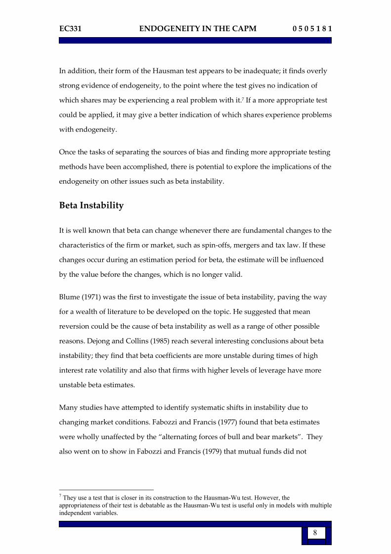
Figure 5 shows the 50-day moving average of the daily index volatility. The vertical

line marks the presence of a structural break at around the 20th of July 2007. This

corresponds fairly well to the date that was chosen to divide the sample, the 13th of

July 2007.

14 This is not intended to be a rigorous investigation into the exact location of the break, only a brief

justification that the sample is divided in a suitable position. 15 Since these two variables are linked, we need only to determine the position of the break in one

variable, with the most appropriate one being the volatility.

Period 1 Period 2 % change

Average Volatility 1.427 2.277 59.566

Index Volatility 0.701 1.463 108.702

Average Liquidity 0.758 0.824 8.707

Average Weighted

Correlation 0.281 0.454 61.566

Average Return 0.057 -0.121 N/A

% days on which

index rises 53.600 50.700 N/A


20

Figure 5: A fifty day moving average of the daily volatility

Daily Index Volatility (Previous 50 days)

0

0.2

0.4

0.6

0.8

1

1.2

1.4

1.6

1.8

25/09/06

25/10/06

25/11/06

25/12/06

25/01/07

25/02/07

25/03/07

25/04/07

25/05/07

25/06/07

25/07/07

25/08/07

25/09/07

25/10/07

25/11/07

25/12/07

Daily v

ola

tility

(%

)

IV.2: SUMMARY STATISTICS

The IV estimates were in every case less than the OLS estimates, confirming that

there exists a positive bias in the beta estimate of every share of the FTSE 100. The

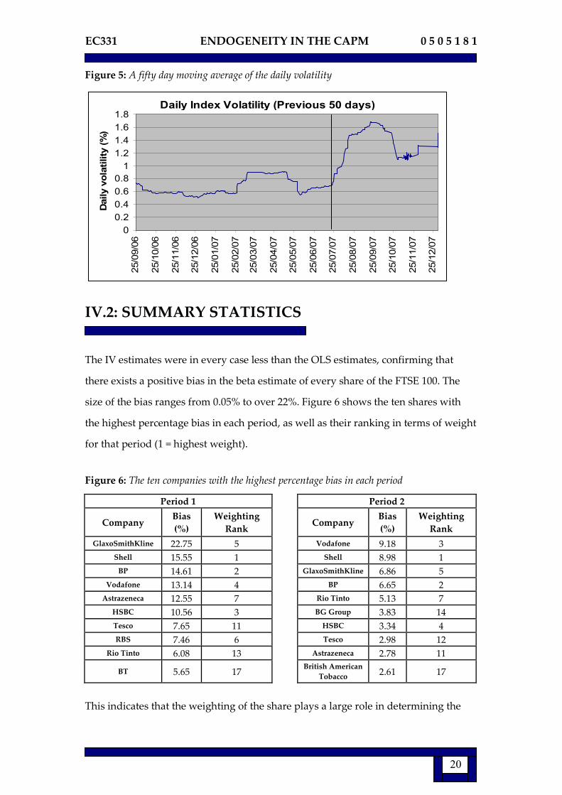
size of the bias ranges from 0.05% to over 22%. Figure 6 shows the ten shares with

the highest percentage bias in each period, as well as their ranking in terms of weight

for that period (1 = highest weight).

Figure 6: The ten companies with the highest percentage bias in each period

Period 1 Period 2

Company Bias

(%)

Weighting

Rank Company

Bias

(%)

Weighting

Rank

GlaxoSmithKline 22.75 5 Vodafone 9.18 3

Shell 15.55 1 Shell 8.98 1

BP 14.61 2 GlaxoSmithKline 6.86 5

Vodafone 13.14 4 BP 6.65 2

Astrazeneca 12.55 7 Rio Tinto 5.13 7

HSBC 10.56 3 BG Group 3.83 14

Tesco 7.65 11 HSBC 3.34 4

RBS 7.46 6 Tesco 2.98 12

Rio Tinto 6.08 13 Astrazeneca 2.78 11

BT 5.65 17 British American

Tobacco 2.61 17

This indicates that the weighting of the share plays a large role in determining the


21

size of the bias; most of the ten highest biases are for shares with the ten highest

weightings. It does show, however, that the weighting is not the only factor affecting

the size of the bias; if it were then there would be no way of accounting for shares

with lower weightings (eg BT in period 1 and British American Tobacco in period 2)

having biases that place them in the top ten.

It is also clear that there exist differences between the biases in each period; the biases

in period 1 were far higher than those observed in period 2. This was not merely a

pattern observed in the largest shares; on average, across all shares, the bias in period

1 was 2.7 times that in period 2. Additionally, in period 1, 39% of shares had a bias of

less than 1%, in period 2 this figure rose to 70%.

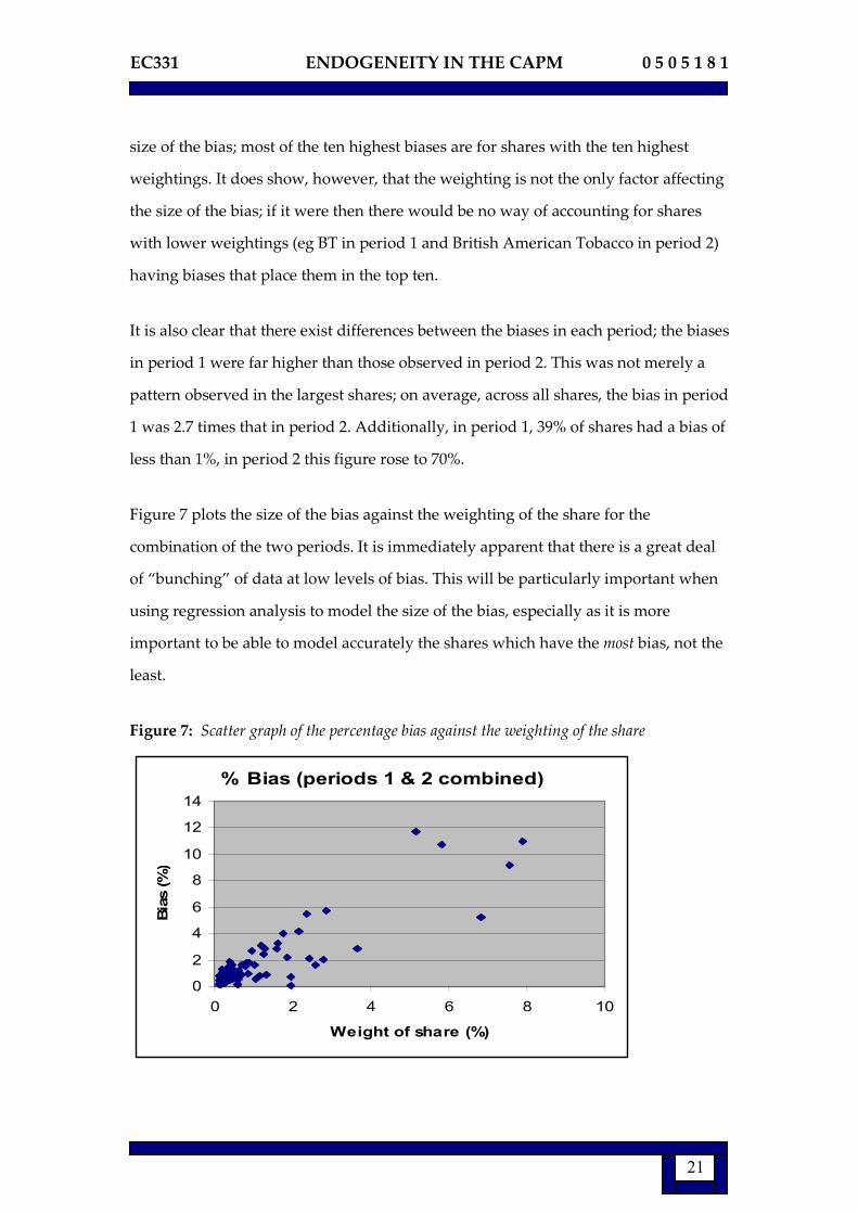
Figure 7 plots the size of the bias against the weighting of the share for the

combination of the two periods. It is immediately apparent that there is a great deal

of “bunching” of data at low levels of bias. This will be particularly important when

using regression analysis to model the size of the bias, especially as it is more

important to be able to model accurately the shares which have the most bias, not the

least.

Figure 7: Scatter graph of the percentage bias against the weighting of the share

% Bias (periods 1 & 2 combined)

0

2

4

6

8

10

12

14

0 2 4 6 8 10

Weight of share (%)

Bia

s (%

)


22

IV.3: HAUSMAN TEST RESULTS

The form of the Hausman test used is only appropriate when the standard error of

the IV estimate is larger than the standard error of the OLS estimate. Of the three

hundred observations (100 shares in period 1, 2 and combined) this condition was

satisfied 98% of the time.

Figure 8: The results of the Hausman test for endogeneity. The table shows the number of

shares for which the null hypothesis is rejected as well as their ranking by weight.

Period 1

(Jul-06 – Jul-07)

Period 2

(Jul-07 – Jan-08)

Combined

(Jul-06 – Jan-08)

Number with endogeneity 29 10 25

Rankings of shares with

evidence of endogeneity.

Ranked by weight in index.

(1=highest weight)

1, 2, 3, 4, 5, 6, 7, 9, 11,

12, 13, 14, 16, 17, 18,

20, 22, 23, 26, 28, 30,

33, 34, 41, 47, 55, 73,

88, 97

1, 2, 3, 5, 11, 15,

17, 21, 22, 40

1, 2, 3, 4, 5, 7, 11, 12,

15, 16, 17, 18, 20, 21,

22, 26, 27, 29, 30, 31,

41, 42, 46, 54, 58

Note: The rejections of the null hypothesis are at the 5% significance level.

We can see that the Hausman test tends to find evidence of endogeneity in shares

with higher weightings and that it supports the finding that endogeneity was far

more prevalent in period 1 than in period 2; the null hypothesis is rejected for 29

shares in period 1 and only ten in period 2.

In period 1, it finds evidence of endogeneity in 80% of the shares with the twenty

highest weightings, which indicates that the test is working somewhat efficiently.

It is worth noting, however, that the test finds evidence of endogeneity in some

shares with a relatively low weighting. For example, in period 1, the Hausman test

finds endogeneity in four shares that are in the bottom half of the index in terms of

weighting.16

16 It is not clear whether this is due to the Hausman test being less than perfect or whether there is a

genuine reason for the rejection of the null hypothesis for these shares.


23

On inspection of the test results for the two periods combined, we can say that if a

share is in the top thirty in terms of weight, then there is a strong chance (around

63%) of the test finding evidence of endogeneity.17

It was noted in section III.4 that this form of the Hausman test is different from that

used by Woo, Cheung and Yan-Ki Ho (1994). When their form of the test is applied

to this dataset, it finds strong evidence of endogeneity in every share of the FTSE 100;

clearly this is not a useful result.18

IV.4: MODELLING THE SIZE OF THE BIAS

It was expected that the two main factors affecting the size of the bias would be the

weight (positive effect) and the weighted average correlation (negative effect).

When considering the optimal functional form of the regression, it became apparent

that including these two variables linearly caused unfavourable results in the

estimation. A preliminary regression was run using only these two main variables:

Preliminary regression with two main variables

BIAS i = α + γ1 weight i + γ2 w.a.c i + ε

17 This figure is a general estimate of the probability and could only be applied to other time periods

with an allowance for a margin of error. 18 One possible reason that this was not perceived as a problem in their study, is that they only looked

at shares that they suspected had biased estimators. They therefore saw these test statistics as evidence

in favour of their selection. However, when using data comprising an entire index, it soon becomes

clear that their form of the test gives very little insight into the problem as by its very construction it

will find evidence of endogeneity in any share.


24

Figure 9: Results of preliminary regression with the two main variables

Period 1 Period 2 Combined

Variable Coefficient T-stat Coefficient T-stat Coefficient T-stat

Intercept 5.136**

(0.619) 8.297

3.236**

(0.408) 7.927

3.936**

(0.476) 8.274

Weight 2.167**

(0.0919) 23.578

1.027**

(0.0399) 25.736

1.357**

(0.0543) 24.975

Average

Correlation

-16.819**

(2.157) -7.794

-6.919**

(0.898) -7.701

-9.897**

(1.254) -7.893

Note: * & ** indicate significance at the 5% and 1% levels respectively

One aspect of the model that is slightly troubling is the intercept coefficient. At 3.936

(for the combined time periods), it stands at a level above 91% of the values.19

Testing has shown that the model performs better over multiple periods by

combining the two variables into a single variable, which in this case is the weighting

divided by the average weighted correlation. Using this variable, along with all

other relevant variables, we arrive at the following model.

Main regression model for the size of the bias

BIAS i = α + γ1 (weight i / w.a.c i)+ γ2 vol i + γ3 liq i + γ4 bank i +

γ5 ind i + γ6 util i + γ7 cs i + γ8 ogbm i + γ9 fin i + ε

For an explanation of the variables see Appendix A

Figure 10 summarises the results

19 Whilst intercepts can be considered to be of little interpretative importance, a regression model of

this form, in which there are two main variables with opposite signs, has the unfortunate tendency to

produce extreme coefficient estimates when using the ordinary least squares method and as such, it will

rarely hold over more than one period.


25

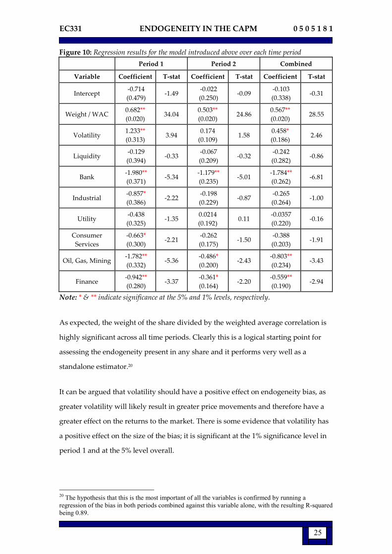
Figure 10: Regression results for the model introduced above over each time period

Period 1 Period 2 Combined

Variable Coefficient T-stat Coefficient T-stat Coefficient T-stat

Intercept -0.714

(0.479) -1.49

-0.022

(0.250) -0.09

-0.103

(0.338) -0.31

Weight / WAC 0.682**

(0.020) 34.04

0.503**

(0.020) 24.86

0.567**

(0.020) 28.55

Volatility 1.233**

(0.313) 3.94

0.174

(0.109) 1.58

0.458*

(0.186) 2.46

Liquidity -0.129

(0.394) -0.33

-0.067

(0.209) -0.32

-0.242

(0.282) -0.86

Bank -1.980**

(0.371) -5.34

-1.179**

(0.235) -5.01

-1.784**

(0.262) -6.81

Industrial -0.857*

(0.386) -2.22

-0.198

(0.229) -0.87

-0.265

(0.264) -1.00

Utility -0.438

(0.325) -1.35

0.0214

(0.192) 0.11

-0.0357

(0.220) -0.16

Consumer

Services

-0.663*

(0.300) -2.21

-0.262

(0.175) -1.50

-0.388

(0.203) -1.91

Oil, Gas, Mining -1.782**

(0.332) -5.36

-0.486*

(0.200) -2.43

-0.803**

(0.234) -3.43

Finance -0.942**

(0.280) -3.37

-0.361*

(0.164) -2.20

-0.559**

(0.190) -2.94

Note: * & ** indicate significance at the 5% and 1% levels, respectively.

As expected, the weight of the share divided by the weighted average correlation is

highly significant across all time periods. Clearly this is a logical starting point for

assessing the endogeneity present in any share and it performs very well as a

standalone estimator.20

It can be argued that volatility should have a positive effect on endogeneity bias, as

greater volatility will likely result in greater price movements and therefore have a

greater effect on the returns to the market. There is some evidence that volatility has

a positive effect on the size of the bias; it is significant at the 1% significance level in

period 1 and at the 5% level overall.

20 The hypothesis that this is the most important of all the variables is confirmed by running a

regression of the bias in both periods combined against this variable alone, with the resulting R-squared

being 0.89.


26

As expected, the liquidity of the share is not a significant variable when estimating

the size of bias in shares from the FTSE 100.21 This evidence is crucial to the results; it

shows that the bias that has been found to exist is not due to differences in liquidity

between shares and therefore allows us to assume that the bias that is present is due

to the endogeneity of market returns.

The sector dummy variables show that there exist differences in the size of the bias

for different market sectors. The regression uses consumer goods companies as its

reference variable and finds that every other market sector has a lower bias than it

does. Looking at the results for period one and two combined, we can see that at the

1% significance level, there are three sectors that have lower biases than would

otherwise have been predicted. These are the finance sector, the energy & mining

sector and the major banks in the FTSE 100.22 One possible explanation for this is that

the firms in these sectors have a far greater correlation to one-another than the firms

in other sectors. This would then increase their average weighted correlation with all

other shares and would therefore decrease the bias.

This explanation fits well with the sectors in question. For example, there are many

reasons why banking shares tend to move together in any time period; if interest

rates change, this is likely to affect all banks in similar ways, whether positive or

negative. The same cannot be said, to the same extent, for the consumer goods sector,

in which the effect is likely to be more firm specific.

Whilst we cannot say for sure whether some sectors have permanently lower biases,

these results provide reliable evidence that the market sector can have an effect on

the size of the bias and should not be ignored.

21 It should be noted that this is in no way considered as evidence that liquidity is not a relevant

variable to consider when looking at the problem of endogeneity in beta estimation in general or on

other exchanges; it is merely a result of choosing the data from an index in which every share is very

liquid and there are only small differences in liquidity between shares. 22 The banks were separated from the rest of the finance sector for two reasons. Firstly the sector as a

whole was very dominant in the index, which could have caused problems in the results. Secondly, the

banks in the FTSE 100 were found to have very different characteristics to the other finance

companies, such as insurance companies, brokerages and financial information providers.


27

IV.5: EFFECT OF BIAS ON BETA STABILITY

General Results

The changes in beta between the two time periods were tested for significance using

a Chow test for both the IV and the OLS estimates for each firm. The percentage

change in the beta estimates was also calculated for the IV and OLS methods in order

to see if the bias affected the size of the change in a systematic or random way.

The OLS and IV estimates agreed on the direction of the change in beta for 98 of the

100 shares. The two shares for which the two techniques did not agree were

Glaxosmithkline and Astrazeneca, two of the largest shares in the index. In the case

of Astrazeneca, the OLS estimate had beta falling by 5.6%, whereas the IV estimate

had beta rising by 3.6%. However, since in these two cases neither of the F-statistics

were significant for either estimation technique, this result is of little interpretative

significance.

At the 5% level, the OLS and IV methods agreed on the significance of changes in

beta between the two periods for 98 of the 100 shares.23 The two shares for which the

two methods disagree are HBOS and Vodafone, which again are two heavily

weighted shares.

In trying to determine the effects of endogeneity on beta stability, it is far more

illustrative to look at the difference in the percentage changes of beta for each

estimation technique. In doing this, it shows whether the OLS estimates have a

consistent bias (upwards or downwards) on beta stability, or whether the direction of

the bias is different for different shares.

23 Looking at which shares have OLS and IV F-statistics that fall on either side of any particular value

(as we just have for F equal to 3.866) is a fairly fruitless endeavour. The F-statistics for every share are

different for the IV and OLS methods and so picking some arbitrary point does not give a good

indication of how the results differ for the two methods.


28

It was found that the percentage change between the OLS estimates for periods 1 and

2 were less than those of the IV estimates in 98 of the one hundred shares. This shows

that the OLS technique gives a consistently downwards bias on beta stability.24

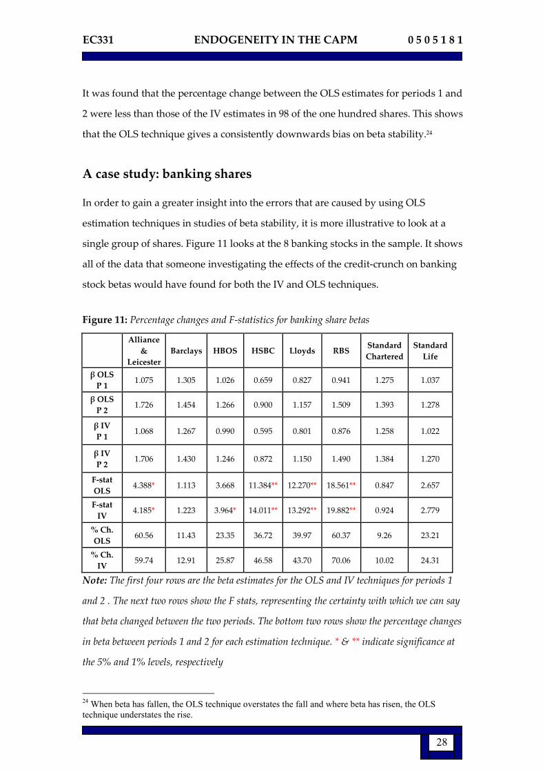
A case study: banking shares

In order to gain a greater insight into the errors that are caused by using OLS

estimation techniques in studies of beta stability, it is more illustrative to look at a

single group of shares. Figure 11 looks at the 8 banking stocks in the sample. It shows

all of the data that someone investigating the effects of the credit-crunch on banking

stock betas would have found for both the IV and OLS techniques.

Figure 11: Percentage changes and F-statistics for banking share betas

Alliance

&

Leicester

Barclays HBOS HSBC Lloyds RBS Standard

Chartered

Standard

Life

β OLS

P 1 1.075 1.305 1.026 0.659 0.827 0.941 1.275 1.037

β OLS

P 2 1.726 1.454 1.266 0.900 1.157 1.509 1.393 1.278

β IV

P 1 1.068 1.267 0.990 0.595 0.801 0.876 1.258 1.022

β IV

P 2 1.706 1.430 1.246 0.872 1.150 1.490 1.384 1.270

F-stat

OLS 4.388* 1.113 3.668 11.384** 12.270** 18.561** 0.847 2.657

F-stat

IV 4.185* 1.223 3.964* 14.011** 13.292** 19.882** 0.924 2.779

% Ch.

OLS 60.56 11.43 23.35 36.72 39.97 60.37 9.26 23.21

% Ch.

IV 59.74 12.91 25.87 46.58 43.70 70.06 10.02 24.31

Note: The first four rows are the beta estimates for the OLS and IV techniques for periods 1

and 2 . The next two rows show the F stats, representing the certainty with which we can say

that beta changed between the two periods. The bottom two rows show the percentage changes

in beta between periods 1 and 2 for each estimation technique. * & ** indicate significance at

the 5% and 1% levels, respectively

24 When beta has fallen, the OLS technique overstates the fall and where beta has risen, the OLS

technique understates the rise.


29

The beta estimates for all eight banking shares went up between periods 1 and 2,

showing that there were differences between the two periods that affected all of the

banks in the same way. The increases were significant at the 5% level for four of the

banks using the OLS technique and five of the banks using the IV technique.

The F-statistics and percentage changes in beta were greater using the IV technique

than the OLS technique for each of the shares except for Alliance & Leicester.25

The average percentage change in beta for the eight shares was 33.1% using the OLS

technique and 36.7% using the IV technique. This represents a proportional error of

10.7%, an error that is likely to be highly significant in any study of the effects of the

credit crunch on banking shares.

Interpreting the results of the beta stability test

It is clear from the evidence above that endogeneity bias can have an effect on studies

of beta stability. However, it is important to address whether these results will

always apply between any two time periods or whether the results found are specific

to the time periods chosen for this study.

In this case, the OLS estimates consistently underestimated the change in beta

between period one and two. However, this is merely a result of the fact that the bias

was far greater in period one. The following examples show how the effect on beta

instability is related to the change in bias between the periods, not the overall level.

25 This was one of only two shares in the sample of 100 in which the OLS percentage change was

higher than the IV percentage change.


30

Examples to show how relative bias affects beta instability

Example 1: Bias is 20% in period 1, 10% in period 2. “True” (IV) beta changes 50%

β1OLS = 1.2 , β1IV = 1.0 β2OLS = 1.65 , β2IV = 1.5

% change (OLS) = ((1.65/1.2)-1)*100% = 37.5%

% change (IV) = ((1.5/1.0)-1)*100% = 50%

As was the case in this study, the OLS technique understates the percentage change

in beta between the two periods

Example 2: Bias is constant at 20%. “True” (IV) beta changes 50%

β1OLS = 1.2 , β1IV = 1.0 , β2OLS = 1.8 , β2IV = 1.5

% change (OLS) = ((1.8/1.2)-1)*100% = 50%

% change (IV) = ((1.5/1.0)-1)*100% = 50%

This shows that when the bias remains constant between two time periods, there is

no bias on the results of a beta stability test.

This study does not therefore make any broad statements about exactly how

endogeneity bias affects beta stability, it only says that it should be borne in mind

that changes in bias over time may have an unwanted effect on the results of a beta

stability study. This is especially relevant as studies of beta stability often focus on

periods of contrasting market conditions, such as a transition from a bull to a bear

market, precisely the time when conditions such as the covariance matrix and

volatility may be shifting and causing changes in the bias.


31

V: CONCLUSIONS AND EXTENSIONS

V.1: CONCLUSIONS

In selecting data from an index in which all shares are highly liquid, this study has

separated the effects of endogeneity bias and other types of bias attributed to

liquidity issues. It finds that the endogeneity of market returns in the CAPM causes a

strong upwards bias on beta estimates when using the OLS estimation technique,

reaching a maximum of over 20% for the most highly weighted shares.

This study has shown that whilst tests such as the Hausman test can be useful in

detecting endogeneity bias in beta estimates, the bias is really only significant when

it would affect the decisions of those who use the CAPM to estimate rates of return

or the cost of equity. Consider the following example:

Example of a Cost of Equity Calculation

Assume that the market risk premium is 10%. A bias of 1% in the beta estimation would

translate into an error in the cost of equity calculation of 10 basis points. This is likely to be

wholly insignificant in investment decisions. However, if the bias is 10%, the error in the cost

of equity calculation is 100 basis points. This is likely to be very significant; it is higher than

the profit margin of many large banks!

This study has found that the size of the bias can be attributed to a few main factors.

Unsurprisingly, the weight of the share in the index is the main factor. However, the

effect that the average weighted correlation of the share with all other shares has is

particularly interesting; it shows that shifts in the covariance matrix (as we saw at the

start of the credit crunch) lead to large changes in the size of the bias that we observe.

This is the variable that leads to the changing bias over time and is therefore the

reason that the bias may have an effect on beta stability.


32

In addition, the volatility was found to have a weak effect on the size of the bias and

crucially, the liquidity of the share was ineffectual on the size of the bias in both

periods. Interestingly, the results also found strong evidence that the size of the bias

in different shares is affected by the market sector in which the firm operates.

Finally, the study found that endogeneity bias can have a significant effect on studies

of beta stability. The effect that it has is related to changes in bias between time

periods rather than the absolute level; if there is a high level of bias but it is constant

over the observation period then it will not have an effect on studies of beta stability.

V.2: LIMITATIONS AND EXTENSIONS

The main limitation to the findings of this study is the fact that they do not contain

data from enough time periods to be applicable to the general case or to be used to

predict current or future biases.

Essentially, the model is likely to be “over-fitted” to the time periods used and

therefore lacks the robustness required to use it to predict biases in other periods. In

addition, the findings on beta stability can only be viewed as proof that endogeneity

has the potential to affect studies of beta stability, not that it always does so.26

It was , however, never the intention of this paper to form a robust model that could

predict levels of endogeneity bias in any time period or to say exactly how past

studies of beta stability have been affected by it. It was only the intention to indicate

that endogeneity bias does exist as a standalone phenomenon, independent of any

form of liquidity related bias and to indicate the effect that this may have on studies

of beta stability. To this extent, it has been relatively successful.

26 For example, if the last 100 years had been split into 100 time periods, we cannot be sure that the two

time periods examined in this study would not have been the only time that endogeneity bias would

have caused problems in the results.


33

The main way to extend the study would be to use data from many more time

periods, which together would represent every market condition and from which, a

usable model could be derived that was capable of predicting the size of the bias in

any market condition. From this, a technique could be found to remove the bias from

OLS beta estimates without having to go to the trouble of calculating an IV estimate.

If such a technique could be developed, it would be a useful tool for anyone who

uses the CAPM to estimate rates of return or the cost of equity.

REFERENCES

M. Blume, “On the assessment of risk”, The Journal of Finance (1971)

M. Blume, “Betas and Their Regression Tendencies”, The Journal of Finance (1975)

E. Dimson; P.R. Marsh, “The Stability of UK Risk Measures and the Problem of Thin

Trading”, The Journal of Finance (1983)

F.J. Fabozzi; J. C. Francis, “Stability Tests for Alphas and Betas Over Bull and Bear Market

Conditions” The Journal of Finance (1977)

F.J. Fabozzi; J.C. Francis “Mutual fund systematic risk for bull and bear markets: an

empirical examination”, The Journal of Finance (1979)

C. Woo; Y. Cheung; R. Yan-Ki Ho, “Endogeneity bias in beta estimation: Thailand

and Hong Kong” Pacific-Basin Finance Journal (1994)

R. Roll, “A critique of the asset pricing theory’s tests”, Journal of Financial Economics

(1977)

G. Woodward; H. Anderson, “Does Beta React to Market Conditions?”, Department of

econometrics, Monash University, Australia

G.J. Alexander; N.L. Chervany, “On the Estimation and Stability of Beta”, The Journal

of Financial and Quantitative Analysis (1980)

K.J. Cohen; G.A. Hawawini; S.F. Maier; R.A. Schwartz; D.K. Whitcomb, “Estimating

and Adjusting for the Intervalling-Effect Bias in Beta”, Management Science (1983)

K.J. Cohen; G.A. Hawawini; S.F. Maier; R.A. Schwartz; D.K. Whitcomb, “Implications

of microstructure theory for empirical research on stock price behaviour”, The Journal of

Finance (1980)


34

P.R. Daves; M.C. Ehrhardt; R.A. Kunkel, “Estimating systematic risk: the choice of

return interval and estimation period”, Journal of Financial and Strategic Decisions

(2000)

T. Berglund; E. Liljeblom; A. Loflund, “Estimating betas on daily data for a small stock

market”, Journal of Banking and Finance (1989)

T.J. Brailsford; T. Josev, “The impact of the return interval on the estimation of systematic

risk” Pacific-Basin Finance Journal (1997)

R. Kolb; R.J. Rodriguez “The Regression Tendencies of Betas: A Reappraisal”, The

Financial Review (1989)

E.F. Fama; K.R. French, “The cross section of expected returns”, The Journal of Finance

(1992)

F. Black, “Beta and return”, Journal of portfolio management (1998)

N.J. Gonedes, “Evidence on the information content of accounting numbers: accounting

based and market based estimates of systematic risk”, Journal of Financial and

Quantitative Analysis (1973)

J.B. Baesel, “On the assessment of risk: some further considerations”, The Journal of

Finance (1974)

J.A. Hausman, “Specification tests in econometrics”, Econometrica (1978)

D.V. Dejong; D.W. Collins, “Explanations for the instability of equity beta: risk free rate

changes and leverage effects”, Journal of Financial and Quantitative Analysis (1985)


35

APPENDICES

A.1: DESCRIPTION OF VARIABLES

Given below is a very brief discussion of the various factors that may be expected to

affect the size of the bias.

The weighting of the share: This should be the most important factor in determining

the size of the bias. The higher the weighting of the share, the more effect it has on

the index returns and therefore the more endogeneity will be present in the estimate.

The covariance matrix: This represents the relationships that the return to the share

has with those of all the other shares. As it has to be captured in a single variable, it is

best represented by the weighted average correlation with all other shares. This is

given by:

weighted average correlation = ρ*j = Σk (ρk j w k), for all k not equal to j.

It is clear that the higher that this variable is, the smaller the bias will be. This is

because when the share is more correlated to all other shares, the consequences of

removing the share from the index (which is essentially what you do when you

calculate an IV estimate) become smaller. As the correlation approaches one, the bias

approaches zero.

The liquidity of the share: The literature has focused heavily on this variable and it

is generally accepted that a lack of liquidity leads to a downwards bias on beta

estimates. However, the reason that the FTSE 100 was selected was to remove the

effects of this bias. For this reason, it would be expected that this variable would be

insignificant in this case. If it were significant, it would detract from the clarity of the

results as thin-trading bias and endogeneity bias are easily confused when both

present.


36

The volatility of the share: This could potentially have an effect on the size of the

bias. As the volatility increases, it is likely that the share will have a greater effect on

the market index as it is likely to experience greater price movements.

The sector in which the firm operates: This could have an effect on the size of the

bias, particularly if there exist higher or lower than average correlations for some

industries. If this is the case then sector dummies will add explanatory power to the

model.

This resulted in the final regression model:

BIAS i = α + γ1 (weight i / w.a.c i)+ γ2 vol i + γ3 liq i + γ4 bank i +

γ5 ind i + γ6 util i + γ7 cs i + γ8 ogbm i + γ9 fin i + ε

A key to the variables is given below:

Weight / w.a.c: This is the weight of the share divided by the average weighted

correlation of the share to all other shares.

Vol: This is the daily volatility of the share over the time period. It is given by the

standard deviation of the daily returns.

Liq: This is the liquidity of the share. It is calculated as the average number of

shares traded per day divided by the total amount outstanding.

Bank: This is the sector dummy variable for the banking sector.

Ind: This is the sector dummy variable for the industrial sector.

Util: This is the sector dummy variable for the utility sector.

Cs: This is the sector dummy variable for the consumer services sector.

Ogbm: This is the sector dummy variable for the oil, gas and basic materials sector.

Fin: This is the sector dummy variable for the finance sector (other than banks).

The sector which was not represented by a sector dummy was the consumer goods

sector.


37

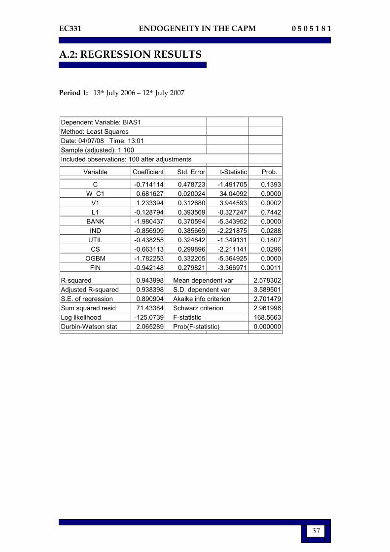
A.2: REGRESSION RESULTS

Period 1: 13th July 2006 – 12th July 2007

Dependent Variable: BIAS1

Method: Least Squares

Date: 04/07/08 Time: 13:01

Sample (adjusted): 1 100

Included observations: 100 after adjustments

Variable Coefficient Std. Error t-Statistic Prob.

C -0.714114 0.478723 -1.491705 0.1393

W_C1 0.681627 0.020024 34.04092 0.0000

V1 1.233394 0.312680 3.944593 0.0002

L1 -0.128794 0.393569 -0.327247 0.7442

BANK -1.980437 0.370594 -5.343952 0.0000

IND -0.856909 0.385669 -2.221875 0.0288

UTIL -0.438255 0.324842 -1.349131 0.1807

CS -0.663113 0.299896 -2.211141 0.0296

OGBM -1.782253 0.332205 -5.364925 0.0000

FIN -0.942148 0.279821 -3.366971 0.0011

R-squared 0.943998 Mean dependent var 2.578302

Adjusted R-squared 0.938398 S.D. dependent var 3.589501

S.E. of regression 0.890904 Akaike info criterion 2.701479

Sum squared resid 71.43384 Schwarz criterion 2.961996

Log likelihood -125.0739 F-statistic 168.5663

Durbin-Watson stat 2.065289 Prob(F-statistic) 0.000000


38

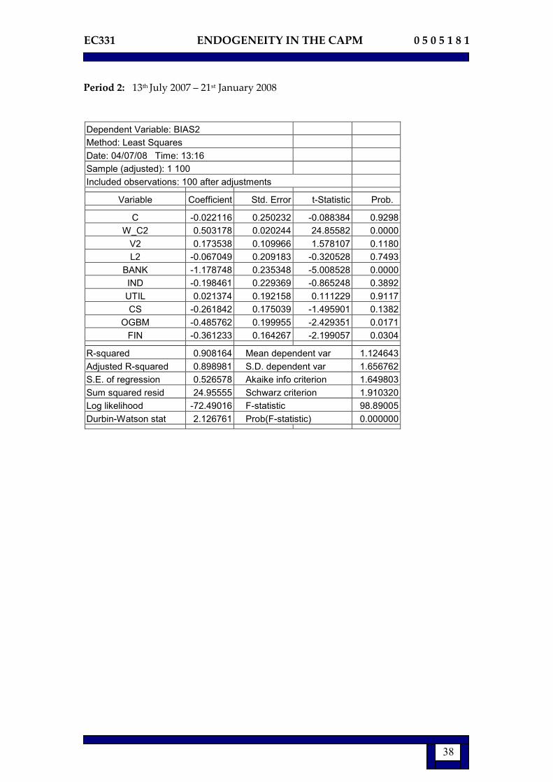
Period 2: 13th July 2007 – 21st January 2008

Dependent Variable: BIAS2


Date: 04/07/08 Time: 13:16




C -0.022116 0.250232 -0.088384 0.9298

W_C2 0.503178 0.020244 24.85582 0.0000

V2 0.173538 0.109966 1.578107 0.1180

L2 -0.067049 0.209183 -0.320528 0.7493

BANK -1.178748 0.235348 -5.008528 0.0000

IND -0.198461 0.229369 -0.865248 0.3892

UTIL 0.021374 0.192158 0.111229 0.9117

CS -0.261842 0.175039 -1.495901 0.1382

OGBM -0.485762 0.199955 -2.429351 0.0171

FIN -0.361233 0.164267 -2.199057 0.0304








39

Periods 1 & 2 combined: 13th July 2006 – 21st January 2008

Dependent Variable: BIAST


Date: 04/07/08 Time: 12:46




C -0.103025 0.337641 -0.305133 0.7610

W_CT 0.566988 0.019863 28.54514 0.0000

VT 0.458202 0.186244 2.460225 0.0158

LT -0.242349 0.282380 -0.858237 0.3930

BANK -1.784626 0.262216 -6.805934 0.0000

IND -0.264561 0.263973 -1.002229 0.3189

UTIL -0.035676 0.219828 -0.162291 0.8714

CS -0.387523 0.202711 -1.911702 0.0591

OGBM -0.803242 0.234242 -3.429108 0.0009

FIN -0.559075 0.190023 -2.942146 0.0041








40

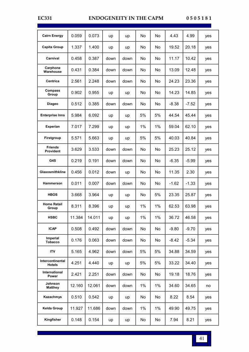
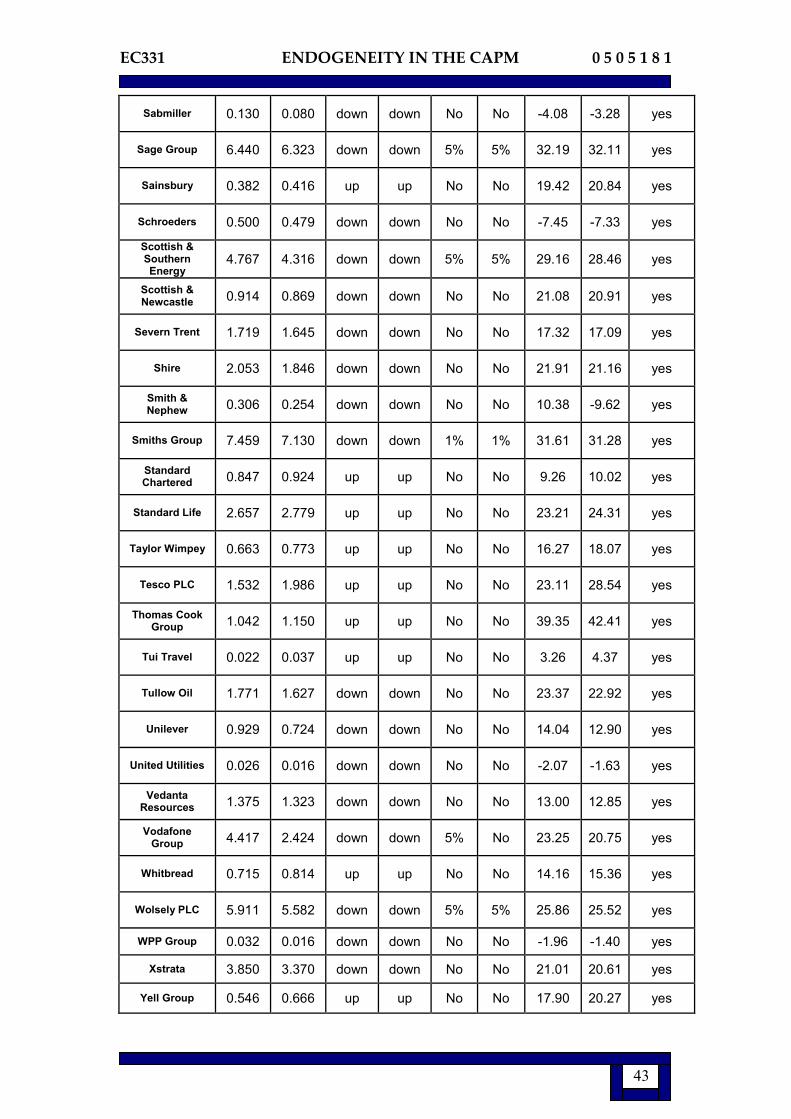
A3: BETA INSTABILITY RESULTS

F Statistics Beta:

up/down? Significant? % changes in beta

OLS IV OLS IV OLS IV OLS IV OLS<IV

3I Group 0.339 0.279 down down No No -6.10 -5.58 yes

Admiral Group 1.870 1.780 down down No No 22.41 22.11 yes

Aliance & Leicester 4.388 4.185 up up 5% 5% 60.51 59.71 no

Amec 0.020 0.027 up up No No 2.62 3.08 yes

Anglo American 0.370 0.211 down down No No -5.51 -4.60 yes

Antofagasta 0.155 0.144 down down No No -4.10 -3.98 yes

Associated British Food 2.309 2.333 up up No No 36.17 36.63 yes

Astrazeneca 0.131 0.039 down up No No -5.68 3.57 yes

Aviva 1.482 1.718 up up No No 12.65 14.03 yes

BskyB Group 0.001 0.009 up up No No 0.71 1.82 yes

BAE Systems 7.401 6.776 down down 1% 1% 32.64 32.21 yes

Barclays 1.113 1.223 up up No No 11.43 12.91 yes

BG Group 1.501 1.314 down down No No 17.25 17.09 yes

BHP Billiton 1.617 0.972 down down No No 10.48 -8.77 yes

BP 1.357 0.167 down down No No 11.85 -5.05 yes

British American Tobacco

0.020 0.001 down down No No -2.40 -0.44 yes

British Land 0.062 0.078 up up No No 3.61 4.13 yes

British Airways 0.060 0.037 down down No No -3.22 -2.57 yes

British Energy 1.109 1.307 up up No No 41.58 47.17 yes

BT Group 0.194 0.412 up up No No 7.12 11.05 yes

Cable & Wireless 1.574 1.424 down down No No 13.95 13.46 yes

Cadbury Schweppes 4.843 5.315 up up 5% 5% 48.38 52.85 yes


41

Cairn Energy 0.059 0.073 up up No No 4.43 4.99 yes

Capita Group 1.337 1.400 up up No No 19.52 20.18 yes

Carnival 0.458 0.387 down down No No 11.17 10.42 yes

Carphone Warehouse 0.431 0.384 down down No No 13.09 12.48 yes

Centrica 2.561 2.248 down down No No 24.23 23.36 yes

Compass Group 0.902 0.955 up up No No 14.23 14.85 yes

Diageo 0.512 0.385 down down No No -8.38 -7.52 yes

Enterprise Inns 5.984 6.092 up up 5% 5% 44.54 45.44 yes

Experian 7.017 7.299 up up 1% 1% 59.04 62.10 yes

Firstgroup 5.571 5.663 up up 5% 5% 40.03 40.84 yes

Friends Provident 3.629 3.533 down down No No 25.23 25.12 yes

G4S 0.219 0.191 down down No No -6.35 -5.99 yes

Glaxosmithkline 0.456 0.012 down up No No 11.35 2.30 yes

Hammerson 0.011 0.007 down down No No -1.62 -1.33 yes

HBOS 3.668 3.964 up up No 5% 23.35 25.87 yes

Home Retail Group 8.311 8.396 up up 1% 1% 62.53 63.98 yes

HSBC 11.384 14.011 up up 1% 1% 36.72 46.58 yes

ICAP 0.508 0.492 down down No No -9.80 -9.70 yes

Imperial Tobacco 0.176 0.063 down down No No -8.42 -5.34 yes

ITV 5.165 4.962 down down 5% 5% 34.88 34.59 yes

Intercontinental Hotels 4.251 4.440 up up 5% 5% 33.22 34.40 yes

International Power 2.421 2.251 down down No No 19.18 18.76 yes

Johnson Matthey 12.160 12.061 down down 1% 1% 34.60 34.65 no

Kazachmys 0.510 0.542 up up No No 8.22 8.54 yes

Kelda Group 11.927 11.686 down down 1% 1% 49.90 49.75 yes

Kingfisher 0.148 0.154 up up No No 7.94 8.21 yes


42

Land Sec 0.650 0.569 down down No No 10.55 10.05 yes

Legal & General 2.127 1.962 down down No No 12.76 12.45 yes

Liberty International 0.008 0.010 up up No No 1.05 1.22 yes

Lloyds TSB 12.270 13.292 up up 1% 1% 39.97 43.70 yes

Lonmin 2.894 2.772 down down No No 18.03 17.87 yes

LSE Group 2.566 2.519 up up No No 41.05 41.22 yes

Man Group 1.191 1.051 down down No No 10.90 10.46 yes

Marks & Spencer 0.701 0.773 up up No No 17.23 18.62 yes

Morrison Supermarkets 3.306 3.601 up up No No 38.25 41.08 yes

National Grid 2.975 2.579 down down No No 26.73 25.87 yes

Next 9.316 9.611 up up 1% 1% 63.40 65.59 yes

Old Mutual 0.224 0.156 down down No No -3.64 -3.09 yes

Pearson 0.453 0.376 down down No No -8.36 -7.71 yes

Persimmon PLC 0.077 0.074 down down No No -4.65 -4.58 yes

Prudential 1.025 1.280 up up No No 9.78 11.32 yes

Reckitt Benckiser 0.142 0.076 down down No No -7.49 -5.73 yes

Reed Elsevier 0.210 0.274 up up No No 6.65 7.74 yes

Rentokil Initial 1.285 1.310 up up No No 25.25 25.72 yes

Resolution 7.564 7.288 down down 1% 1% 40.93 40.78 yes

Reuters Group 12.555 11.409 down down 1% 1% 54.14 53.19 yes

Rexam 2.011 4.447 up up No No 24.78 40.50 yes

Rio Tinto 0.153 0.093 down down No No -5.05 -4.43 yes

Rolls-Royce Group 4.431 4.146 down down 5% 5% 22.31 21.95 yes

Royal Bank of Scotland 18.561 19.882 up up 1% 1% 60.37 70.06 yes

Royal Dutch Shell 0.921 0.146 down down No No 10.49 -5.10 yes

Royal Sun Aliance 0.085 0.065 down down No No -2.87 -2.53 yes


43

Sabmiller 0.130 0.080 down down No No -4.08 -3.28 yes

Sage Group 6.440 6.323 down down 5% 5% 32.19 32.11 yes

Sainsbury 0.382 0.416 up up No No 19.42 20.84 yes

Schroeders 0.500 0.479 down down No No -7.45 -7.33 yes

Scottish & Southern Energy

4.767 4.316 down down 5% 5% 29.16 28.46 yes

Scottish & Newcastle 0.914 0.869 down down No No 21.08 20.91 yes

Severn Trent 1.719 1.645 down down No No 17.32 17.09 yes

Shire 2.053 1.846 down down No No 21.91 21.16 yes

Smith & Nephew 0.306 0.254 down down No No 10.38 -9.62 yes

Smiths Group 7.459 7.130 down down 1% 1% 31.61 31.28 yes

Standard Chartered 0.847 0.924 up up No No 9.26 10.02 yes

Standard Life 2.657 2.779 up up No No 23.21 24.31 yes

Taylor Wimpey 0.663 0.773 up up No No 16.27 18.07 yes

Tesco PLC 1.532 1.986 up up No No 23.11 28.54 yes

Thomas Cook Group 1.042 1.150 up up No No 39.35 42.41 yes

Tui Travel 0.022 0.037 up up No No 3.26 4.37 yes

Tullow Oil 1.771 1.627 down down No No 23.37 22.92 yes

Unilever 0.929 0.724 down down No No 14.04 12.90 yes

United Utilities 0.026 0.016 down down No No -2.07 -1.63 yes

Vedanta Resources 1.375 1.323 down down No No 13.00 12.85 yes

Vodafone Group 4.417 2.424 down down 5% No 23.25 20.75 yes

Whitbread 0.715 0.814 up up No No 14.16 15.36 yes

Wolsely PLC 5.911 5.582 down down 5% 5% 25.86 25.52 yes

WPP Group 0.032 0.016 down down No No -1.96 -1.40 yes

Xstrata 3.850 3.370 down down No No 21.01 20.61 yes

Yell Group 0.546 0.666 up up No No 17.90 20.27 yes

ENDOGENEITY IN THE CAPM - Trade2Win€¦ · ENDOGENEITY IN THE CAPM Can OLS regression yield...

Documents

Transcript of ENDOGENEITY IN THE CAPM - Trade2Win€¦ · ENDOGENEITY IN THE CAPM Can OLS regression yield...