Emulating maize yields from global gridded crop models using

statistical estimatesElodie Blanc and Benjamin Sultan

Report No. 279March 2015

The MIT Joint Program on the Science and Policy of Global Change combines cutting-edge scientific research with independent policy analysis to provide a solid foundation for the public and private decisions needed to mitigate and adapt to unavoidable global environmental changes. Being data-driven, the Program uses extensive Earth system and economic data and models to produce quantitative analysis and predictions of the risks of climate change and the challenges of limiting human influence on the environment—essential knowledge for the international dialogue toward a global response to climate change.

To this end, the Program brings together an interdisciplinary group from two established MIT research centers: the Center for Global Change Science (CGCS) and the Center for Energy and Environmental Policy Research (CEEPR). These two centers—along with collaborators from the Marine Biology Laboratory (MBL) at Woods Hole and short- and long-term visitors—provide the united vision needed to solve global challenges.

At the heart of much of the Program’s work lies MIT’s Integrated Global System Model. Through this integrated model, the Program seeks to: discover new interactions among natural and human climate system components; objectively assess uncertainty in economic and climate projections; critically and quantitatively analyze environmental management and policy proposals; understand complex connections among the many forces that will shape our future; and improve methods to model, monitor and verify greenhouse gas emissions and climatic impacts.

This reprint is one of a series intended to communicate research results and improve public understanding of global environment and energy challenges, thereby contributing to informed debate about climate change and the economic and social implications of policy alternatives.

Ronald G. Prinn and John M. Reilly, Program Co-Directors

For more information, contact the Program office: MIT Joint Program on the Science and Policy of Global Change

Postal Address: Massachusetts Institute of Technology 77 Massachusetts Avenue, E19-411 Cambridge, MA 02139 (USA)

Location: Building E19, Room 411 400 Main Street, Cambridge

Access: Tel: (617) 253-7492 Fax: (617) 253-9845 Email: globalchange@mit.edu Website: http://globalchange.mit.edu/

Emulating maize yields from global gridded crop models using statistical estimates

Elodie Blanc* and Benjamin Sultan†

Abstract

This study estimates statistical models emulating maize yield responses to changes in temperature and precipitation simulated by global gridded crop models. We use the unique and newly-released Inter-Sectoral Impact Model Intercomparison Project Fast Track ensemble of global gridded crop model simulations to build a panel of annual maize yields simulations from five crop models and corresponding monthly weather variables for over a century. This dataset is then used to estimate statistical relationships between yields and weather variables for each crop model. The statistical models are able to closely replicate both in- and out-of-sample maize yields projected by the crop models. This study therefore provides simple tools to predict gridded changes in maize yields due to climate change at the global level. By emulating crop yields for several models, the tools will be useful for climate change impact assessments and facilitate evaluation of crop model uncertainty.

Contents 1. INTRODUCTION .................................................................................................................... 22. MATERIAL AND METHODS ............................................................................................... 3

2.1 Data ................................................................................................................................. 3  2.1.1 Crop Yields and Growing Seasons ........................................................................ 3  2.1.2 Weather ................................................................................................................. 4  2.1.3 Sample Summary Information and Statistics ........................................................ 6  

2.2 Methods ........................................................................................................................... 8  3. RESULTS ................................................................................................................................. 9

3.1 Model Selection ............................................................................................................. 10  3.2 Regression Results ........................................................................................................ 12  

4. VALIDATION ....................................................................................................................... 124.1 In-sample Validation ..................................................................................................... 13  4.2 Out-of-Sample Validation ............................................................................................. 21  

5. ROBUSTNESS CHECKS ...................................................................................................... 245.1 Dependent Variable Transformation ............................................................................. 24  5.2 Growing Seasons ........................................................................................................... 25  5.3 Parameter Heterogeneity ............................................................................................... 26  

5.3.1 Global Agro-Ecological Zones ........................................................................... 26  5.3.2 Average Summer Temperature Brackets ............................................................. 27  

6. CONCLUDING REMARKS ................................................................................................. 287. REFERENCES ....................................................................................................................... 29APPENDIX A. REGRESSION RESULTS ............................................................................... 33  APPENDIX B. FIXED EFFECTS (δ) BY SPECIFICATION AND CROP MODEL .............. 33  APPENDIX C. TEMPERATURE AND PRECIPITATION EFFECT FROM THE S1INT SPECIFICATION ........................................................................................................... 34  APPENDIX D ............................................................................................................................ 39  

* Corresponding author (Email: eblanc@mit.edu). Joint Program on the Science and Policy of Global Change,Massachusetts Institute of Technology, MA, USA.

† Université Pierre et Marie Curie, Paris, France.

2

1. INTRODUCTION

The impact of climate change on crop yields has been extensively studied. To estimate theseimpacts, two approaches are usually taken: (i) process-based crop models, which represent mechanistically or functionally the effect of weather, soil conditions, management practices and abiotic stresses on crop growth and yields; or (ii) statistical techniques that empirically estimate the effect of weather on crop yields while controlling for other factors based on historical observations.

Process-based crop models are able to consider the detailed effect of weather and climate change on crop yields at the global level or at the site level by considering monthly, daily, or even hourly weather information (Basso et al., 2013). Some models can also capture other factors, such as pest damages, soil properties, fertilizer application, planting dates, and the carbon dioxide (CO2) fertilization effect. These models are either calibrated at the field scale (Izaurralde et al., 2006; Elliott et al., 2013; Jones et al., 2003), the national level (Bondeau et al., 2007) or the grid cell level across the globe (Deryng et al., 2011). These models can simulate a wide range of weather and environmental conditions, but are computationally demanding and sometimes proprietary, which limits their accessibility.

Statistical models, usually in the form of regression analysis, on the other hand, use observed data to estimate the impact of weather on crop yields and are usually based on data aggregated by month (Carter and Zhang, 1998), growth stage (Dixon et al., 1994) or year (Blanc, 2012; Schlenker and Lobell, 2010). Regression analyses usually consider the effect of temperature and precipitation on crop yields (Lobell and Field, 2007; Nicholls, 1997; Corobov, 2002) and its derived composites, such as growing degree days (GDD) (Lobell et al., 2011), evapotranspiration (Blanc, 2012), and drought indices (Lobell et al., 2014; Blanc, 2012; Carter and Zhang, 1998). Some studies control for alternative effects, such as cloud cover (You et al., 2009); sources of water availability, such as proximity to streams (Blanc and Strobl, 2014) and dams (Strobl and Strobl, 2010; Blanc and Strobl, 2013); management strategies, such as fertilizer application (Cuculeanu et al., 1999) or changes in planting dates (Alexandrov and Hoogenboom, 2000); and technological trends (Lobell and Field, 2007). The ability of these models to provide large-scale yields estimates is limited by data availability, and they are thus generally based on crop yield data averaged globally (Lobell and Field, 2007), at the country level (Blanc, 2012; Schlenker and Lobell, 2010), or at the county level (Lobell and Asner, 2003).

The out-of-sample predictive ability of statistical models is a concern when estimating impacts for scenarios of climate change not previously observed. This issue has been considered in recent studies by Holzkämper et al. (2012) and Lobell and Burke (2010) using the so-called ‘perfect model’ approach, which consists of training a statistical model on the output of a process-based crop model, assuming that this output is ‘true’. The main aim of these studies is to evaluate the ability of statistical models to provide predictions out-of-sample. They find that statistical models are capable of replicating the outcomes of process-based crop models reasonably well. The spatial and temporal scope of these studies is, however, fairly small. Oyebamiji et al. (2015) expand on these studies and estimate an empirical crop yield emulator at

3

the global level for five different crops but, as in previous studies, they only consider one process-based crop model. This is a concern because the choice of crop model is an important source of uncertainty in climate change impact assessments on crop yields (e.g. Mearns et al., 1999; Bassu et al., 2014). Therefore, having access to a tool capable of replicating yields from a wide ensemble of crop models would facilitate the analysis of crop model uncertainty in climate change impact assessments.

To address the limitations of simulations based on processed-based models and to consider crop model uncertainty, we design an ensemble of simple statistical models able to accurately replicate the outcomes of process-based crop models at the grid cell level over the globe using only a limited set of weather variables. To this end, we use the recently released Inter-Sectoral Impact Model Intercomparison Project (ISI-MIP) Fast Track experiment dataset of global gridded crop models (GGCM) simulations. This project was coordinated by the Agricultural Model Intercomparison and Improvement Project (AgMIP) (Rosenzweig et al., 2013) as part of ISI-MIP (Warszawski et al., 2014). To enable comparison across models, all GGCMs are driven with consistent bias-corrected climate change projections derived from the Coupled Model Intercomparison Project, phase 5 (CMIP5) archive (Hempel et al., 2013, Taylor et al., 2012). Our statistical models are trained on the crop yields simulated by these process-based crop models and are subject to the widest range of climate conditions estimated in CMIP5. The statistical models are then used to predict the spatial responses of maize yields to weather. Differences between predictions from the process-based and statistical models are then assessed in order to measure how well statistical models can capture yield responses to weather variations driven by climate change.

This paper has five further sections. Section 2 presents the data and methods used to statically estimate relationship between yields and weather variables. Results are presented and discussed in Section 3. The models are validated in Section 4 and sensitivity analyses are performed in Section 5. Section 6 concludes.

2. MATERIAL AND METHODS

2.1 Data

Data used in this study are sourced from the ISI-MIP Fast Track experiment, an inter-comparison exercise of global gridded process-based crop models using the CMIP5 climate simulations.1 In this exercise, several modeling groups provided results from global gridded process-based crop models run under the same set of weather and CO2 concentration inputs.

2.1.1 Crop Yields and Growing Seasons Crop yields and growing season information are obtained from GGCMs members of the

ISI-MIP Fast Track experiment. Based on data availability, we consider five crop models: the Geographic Information System (GIS)-based Environmental Policy Integrated Climate (GEPIC) model (Williams, 1995; Liu et al., 2007), the Lund Potsdam-Jena managed Land (LPJmL)

1 The data are available for download at https://www.pik-potsdam.de/research/climate-impacts-and-

vulnerabilities/research/rd2-cross-cutting-activities/isi-mip/data-archive/fast-track-data-archive.

4

dynamic global vegetation and water balance model (Bondeau et al., 2007; Waha et al., 2012), the Lund-Potsdam-Jena General Ecosystem Simulator (LPJ-GUESS) with managed land model (Bondeau et al., 2007; Smith et al., 2001; Lindeskog et al., 2013), the parallel Decision Support System for Agro-technology Transfer (pDSSAT) model (Elliott et al., 2013; Jones et al., 2003), and the Predicting Ecosystem Goods And Services Using Scenarios (PEGASUS) model (Deryng et al., 2011).

Each GGCM simulation provides estimates of annual maize yields in metric tons (t) per hectare (ha), as well as planting and maturity dates, at a 0.5×0.5 degree resolution (about 50km2). For each of these models, we select model simulations considering the effect of CO2 concentration in order to account for CO2 fertilization effect, which plays an important role in biomass production. Also, we consider simulations assuming no irrigation in order to capture the effect of precipitation on crop yields.

GGCMs differ in their representation of crop phenology, leaf area development, yield formation, root expansion and nutrient assimilation. However, they all account for the effect of water, heat stress and CO2 fertilization. None of the models considered assume technological change. A more detailed description of each model’s processes is provided by Rosenzweig et al. (2014). Some caveats are associated with each model.2 For instance, the LPJ-GUESS model estimates potential yields (yield non-limited by nutrient or management constraints) rather than actual yield and therefore only relative change should be considered when assessing the impact of climate change on crop yield using this model. Also, the GEPIC model accounts for soil fertility erosion, which requires the simulations to be run independently for each decade, while the pDSSAT model only updates CO2 inputs every 30 years, which results in a periodic step in yield projections. As a result, these GGCM simulations are more suited to assess long-term trends in yields rather than inter-annual yield variability.

2.1.2 Weather Bias-corrected weather data used as input into each crop model are obtained from the CMIP5

climate data simulations. This study uses daily weather data for three of the five climate models, or General Circulation Models (GCMs) included in CMIP5: HadGEM2-ES, NorESM1-M, and GFDL-ESM2M. As summarized in Warszawski et al. (2014), these GCMs project, respectively, high, medium and low level of global warming.

GCM simulations are available for an ‘historical’ period of 1975 to 2005 and a ‘future’ period of 2006 to 2099. For the ‘future’ period, each GCM is run under four Representative Concentration Pathways (RCPs), each representative of different level of radiative forcing (RCP 2.6, RCP 4.5, RCP 6.0 and RCP 8.5). We selected the scenario with the highest level of global warming compared to historical conditions, RCP 8.5, and the corresponding CO2 concentrations data (Riahi et al., 2007).3 As the maximum amount of warming induced under other RCPs is encompassed in

2 These caveats are discussed at https://www.pik-potsdam.de/research/climate-impacts-and-

vulnerabilities/research/rd2-cross-cutting-activities/isi-mip/data-archive/fast-track-data-archive/data-caveats. 3 The data are available at http://tntcat.iiasa.ac.at/RcpDb/dsd?Action=htmlpage&page=welcome.

5

this pathway, and a wide range of climate change patterns are represented by the three GCMs, the analyses consider the broadest possible range of climate change.

Each GCM produces three variables that are used as inputs by crop models: daily minimum soil surface temperature (Tmin), daily maximum soil surface temperature (Tmax), and daily precipitation (Pr). We compute various composite variables based on these weather variables (which are summarized in Table 1). Mean daily temperature (Tmean) is calculated as:

Tmean = (Tmin + Tmax)/2 (1) We also consider reference evapotranspiration (ETo) to represent the evaporative demand of

the air. Following Hargreaves and Samani (1985), it is calculated daily as: ETo = 0.0023 (Tmean + 17.8) (Tmax – Tmin)0.5 Ra (2)

where Ra is the extraterrestrial radiation calculated as a function of the latitude and time of the year (Allen et al., 1998). GDD represents the number of growing degree days beneficial for the plant. This measure is calculated daily as:

GDD = (Tmin + Tmax)/2 – Tbase (3) where Tbase, the base temperature for maize, is 8°C (Asseng et al., 2012).

To facilitate a simple relationship between annual crop yields and weather variables, monthly averages are calculated for Tmean, Tmin, Tmax, Pr and ETo; GDD is aggregated over each month. The variable N_pr0 represents the proportion of days in a month with no precipitation (Pr = 0). Similarly, N_Tmin0 and N_Tmax30 represent the proportion of days per month with minimum daily temperature below 0°C (Tmin < 0) and maximum daily temperature above 30°C (Tmax > 30). The threshold of 0°C is chosen to capture the effect of frost and the threshold of 30°C is used to capture the temperature above which maize development is affected (Asseng et al., 2012).

Table 1. Variables used in the statistical analysis.

Variable Description Unit Yields Annual crop yields t/ha Pr Monthly average daily precipitation mm/day Tmin Monthly average daily minimum temperature °C Tmax Monthly average daily maximum temperature °C Tmean Monthly average daily mean temperature °C N_Pr0 Ratio of number of days per month without precipitation (daily Pr=0) Ratio N_Tmin0 Ratio of number of days per month with minimum daily temperature below 0°C Ratio N_Tmax30 Ratio of number of days per month with maximum daily temperature above 30°C Ratio ETo Monthly average daily reference evapotranspiration mm/day GDD Monthly heat accumulation °C CO2 Mid-year CO2 concentration ppm

6

2.1.3 Sample Summary Information and Statistics We consider crop model simulations from 1975 to 2005 for the historical runs, and 2006 for

the future period. As only one RCP scenario is selected for each GCM, the panel spans from 1975–2099 without distinction (i.e., for each GCM, there is one historical scenario and one future scenario). In the final sample, we omit grid cells for which there are less than 10 yield observations after data cleaning.

As summarized in Table 2, each GGCM has a sample of more than 13 million observations covering more than 50,000 grid cells globally. When considering the planting dates and growing season length for each sample, the growing seasons averaged over grid cells spread between June and October in the Northern Hemisphere and December and May in the Southern Hemisphere, but differ slightly for each crop model.

Table 2. GGCMs summary information.

Model Observations Grid Cells Growing season (calendar months)

Northern Hemisphere Southern Hemisphere GEPIC 21,545,220 62,005 6-9 12-3 LPJ-GUESS 19,819,086 56,620 6-10 12-5 LPJmL 21,547,956 62,148 5-10 12-4 pDSSAT 15,226,693 50,766 5-8 10-12 PEGASUS 13,404,091 51,568 6-9 12-4

Note: For the pDSSAT model, information regarding planting dates is only available for the HadGEM2-ES GCM. The average growing season for each hemisphere starts on the mean planting month and lasts the mean growing season length (calculated as the period between the planting date and the maturity date).

Summary statistics for each GGCM and GCM are presented in Table 3. Global average maize yields vary from 1.42t/ha for the LPJmL model under the GFDL-ESM2M GCM to 3.00t/ha for the pDSSAT model under the NorESM1-M GCM. The range of yields across GGCMs is smallest for the LPJ-GUESS model and is largest for the PEGASUS model.

Summary statistics for the main weather variables (Tmean and Pr) differ by crop model due to their difference in spatial repartition (i.e., a different number of grid cells are represented by each crop model). As described in the next section, we consider weather variables over the summer months to represent the growing season. In the table, numbers suffixes are used to represent each summer month, so _1, _2 and _3 refer to, respectively, June, July and August in the Northern Hemisphere, and December, January and February in the Southern Hemisphere. In all GGCMs, precipitation is the lowest in the first month of the growing season and highest in the last month, and temperatures peak in the second month. While no clear pattern amongst GCMs is discernable from these statistics for precipitation, temperatures are clearly the highest under the HadGEM2-ES GCM and the lowest under the GFDL-ESM2M GCM.

7

Table 3. Summary statistics by GGCM and GCM.

Model Variable GFDL-ESM2M HadGEM2-ES NorESM1-M Mean St dev Min Max

Mean St dev Min Max

Mean St dev Min Max

GEPIC

Yield 1.85 2.04 0 14.66

1.70 1.73 0 12.29

1.93 1.99 0 12.76

Pr_1 3.06 3.91 0 147.08

2.97 3.69 0 152.08

2.95 3.61 0 157.16

Pr_2 3.42 4.23 0 175.98

3.43 4.34 0 174.54

3.41 3.97 0 188.96

Pr_3 3.43 4.20 0 127.33

3.43 4.16 0 112.80

3.47 3.92 0 102.28

Tmean_1 21.01 9.01 -3.72 45.10

22.00 8.86 -4.85 46.82

21.29 8.81 -4.02 43.65

Tmean_2 22.79 7.73 -0.67 45.25

23.77 7.78 -0.84 47.32

23.35 7.24 -1.34 44.96

Tmean_3 22.02 8.20 -1.48 45.89

23.00 8.18 -3.98 46.68

22.30 7.82 -2.98 44.97

LPJ-GUESS

Yield 1.77 1.65 0 10.34

1.84 1.62 0 10.80

1.96 1.73 0 9.71

Pr_1 3.01 3.63 0 147.08

2.84 3.43 0 152.08

2.83 3.32 0 135.68

Pr_2 3.33 3.94 0 175.98

3.26 3.95 0 174.54

3.27 3.66 0 188.96

Pr_3 3.30 3.94 0 127.33

3.23 3.85 0 112.80

3.31 3.66 0 102.28

Tmean_1 21.74 8.46 -3.54 45.02

22.62 8.62 -5.92 46.82

21.78 8.48 -6.22 43.65

Tmean_2 23.44 7.27 -0.51 45.25

24.40 7.53 -2.10 47.32

23.83 6.94 -1.89 44.96

Tmean_3 22.64 7.77 -0.29 45.89

23.57 7.98 -3.83 46.68

22.69 7.61 -4.77 44.97

LPJmL

Yield 1.42 1.80 0 17.40

1.53 1.75 0 17.66

1.56 1.84 0 17.24

Pr_1 3.13 3.99 0 147.08

2.93 3.70 0 152.08

2.95 3.63 0 157.16

Pr_2 3.47 4.32 0 175.98

3.38 4.36 0 174.54

3.39 3.99 0 188.96

Pr_3 3.48 4.29 0 127.33

3.38 4.17 0 112.80

3.45 3.95 0 102.28

Tmean_1 22.38 8.26 -2.43 45.10

22.93 8.55 -2.54 46.82

22.20 8.32 -4.02 43.65

Tmean_2 23.97 7.11 -0.20 45.25

24.64 7.44 -0.35 47.32

24.14 6.79 -1.34 44.96

Tmean_3 23.26 7.57 0.93 45.89

23.90 7.86 -1.35 46.68

23.11 7.45 -1.58 44.97

pDSSAT

Yield 2.70 2.60 0 24.07

2.94 2.46 0 23.93

3.00 2.70 0 23.84

Pr_1 3.56 4.18 0 147.08

3.36 3.85 0 152.08

3.40 3.81 0 157.16

Pr_2 3.88 4.53 0 175.60

3.83 4.62 0 158.49

3.84 4.23 0 188.96

Pr_3 3.86 4.52 0 127.33

3.78 4.42 0 112.80

3.87 4.19 0 102.28

Tmean_1 23.55 6.90 0.02 44.73

24.45 6.94 2.85 46.82

23.76 6.55 0.77 43.65

Tmean_2 24.88 5.91 4.29 44.53

25.95 5.91 6.07 45.92

25.28 5.40 3.65 44.23

Tmean_3 24.33 6.24 5.38 44.86

25.32 6.25 3.29 46.68

24.53 5.83 4.85 43.77

PEGASUS

Yield 1.83 2.64 0 34.64

1.69 2.32 0 34.44

2.00 2.82 0 34.91

Pr_1 3.84 4.26 0 147.08

3.52 3.90 0 152.08

3.52 3.81 0 135.68

Pr_2 4.14 4.59 0 175.98

4.00 4.64 0 174.54

4.00 4.19 0 188.96

Pr_3 4.12 4.56 0 127.33

3.96 4.43 0 112.08

4.03 4.13 0 102.28

Tmean_1 23.63 6.06 6.14 44.90

24.14 6.42 4.81 46.04

23.57 6.03 3.75 43.37

Tmean_2 24.95 5.00 9.41 44.50

25.77 5.23 10.23 45.90

25.20 4.71 10.26 44.71

Tmean_3 24.35 5.33 8.77 44.59

25.01 5.61 7.92 46.68

24.21 5.30 6.85 43.99

Note: suffixes _1, _2, _3 denote, respectively, June, July and August in the Northern Hemisphere and December January and February in the Southern Hemisphere.

8

2.2 Methods

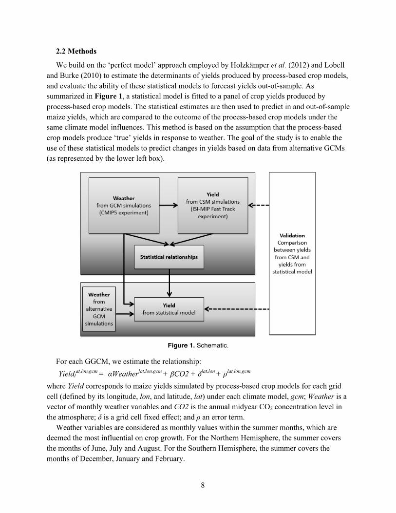
We build on the ‘perfect model’ approach employed by Holzkämper et al. (2012) and Lobell and Burke (2010) to estimate the determinants of yields produced by process-based crop models, and evaluate the ability of these statistical models to forecast yields out-of-sample. As summarized in Figure 1, a statistical model is fitted to a panel of crop yields produced by process-based crop models. The statistical estimates are then used to predict in and out-of-sample maize yields, which are compared to the outcome of the process-based crop models under the same climate model influences. This method is based on the assumption that the process-based crop models produce ‘true’ yields in response to weather. The goal of the study is to enable the use of these statistical models to predict changes in yields based on data from alternative GCMs (as represented by the lower left box).

Figure 1. Schematic.

For each GGCM, we estimate the relationship: Yieldl

at,lon,gcm = αWeatherlat,lon,gcm + βCO2 + δlat,lon + ρlat,lon,gcm (4) where Yield corresponds to maize yields simulated by process-based crop models for each grid cell (defined by its longitude, lon, and latitude, lat) under each climate model, gcm; Weather is a vector of monthly weather variables and CO2 is the annual midyear CO2 concentration level in the atmosphere; δ is a grid cell fixed effect; and ρ an error term.

Weather variables are considered as monthly values within the summer months, which are deemed the most influential on crop growth. For the Northern Hemisphere, the summer covers the months of June, July and August. For the Southern Hemisphere, the summer covers the months of December, January and February.

9

Variables included in the regression specifications are listed in Table 4. The base specification is composed of five sets of explanatory variables, which are denoted S1 to S5. The S1 specification includes ‘simple’ weather variables, and more complicated composite variables are added in subsequent specifications. For each specification, we also include quadratic terms for each parameter to represent the non-linear effects of the weather variables on crop yields (specifications S1sq to S5sq). In an additional set of specifications, we add an interaction term between temperature and precipitation variables to the simple and quadratic variables (specifications S1int to S5int).

Table 4. Specification description.

Specification name

Base specification Variables added to the base specification Non-linear (sq) Interaction (int)

S1 Pr, Tmean, CO2 Pr_sq, Tmean_sq, CO2_sq Pr_x_Tmean S2 Pr, Tmin, Tmax, CO2 Pr_sq, Tmin_sq, Tmax_sq, CO2_sq Pr_x_Tmean

S3 Pr, N_Pr0, Tmean, N_Tmin0, N_Tmax30, CO2

Pr_sq, N_Pr0_sq, N_Tmin0_sq, N_Tmax30_sq, CO2_sq

Pr_x_Tmean

S4 Pr, ETo, CO2 Pr_sq, ETo_sq, CO2_sq Pr_x_ETo S5 Pr, GDD, CO2 Pr_sq, GDD_sq, CO2_sq Pr_x_GDD

Some adjustments to the specifications presented above are made for some crop models. For

instance, the pDSSAT model accounts for the CO2 fertilization effect, but the CO2 level input into this model is only updated every 30 years (as opposed to every year for other crop models considered). For this model, we therefore consider the CO2_30y variable, which averages CO2 concentration over 30 year periods (1950–79, 1980–2009, etc.) instead of the annual CO2 variable. Also, the GEPIC model is run independently every decade to take into account soil nutrient depletion, so we include a dummy variable to capture 10-year cycles in the regression specification for this model.4

As multiple observations exist for each year and grid cell, due to the different climate scenarios considered, and grid cell fixed effects (δ) are included in all specifications, we use the areg OLS estimator in Stata 12 (StataCorp, 2011), which allows for the absorption of categorical variables. Estimated values for δ for each specification and crop model are provided in Appendix B to allow the application of the statistical models to alternative climate change scenarios.

3. RESULTS

Based on the methodology presented Section 2, we estimate three specifications for each crop model. We then determine the preferred specification in Section 3.1 and present detailed results for this specification in Section 3.2.

4 Harvesting in low-input regions leads to soil nutrient depletion, which causes ever-decreasing yields. In order to

avoid this in practice, farmers leave land fallow to allow the soils to recover. This pattern is mimicked in the GEPIC model by re-running the model for every decade to reset the soil profile.

10

3.1 Model Selection

In Error! Reference source not found., we report statistics from the estimation of regressions for each GGCM and specification. For all GGCMs, the adjusted R2 (R̄2) shows that between 69% (pDSSAT) and 91% (LPJ-GUESS) of the changes in yields are explained by the statistical models. The table also reports the root mean square error (RMSE) for each crop model. These statistics indicate that the average error between predicted and ‘actual’ yields range from 0.5t/ha for the LPJ-GUESS model to 1.3t/ha for the PEGASUS and pDSSAT models. In relative terms, however, the normalized RMSE (NRMSE), which is calculated by dividing the RMSE by the difference between maximum and minimum yields, indicates that those errors represent around 5% of maize yields for the LPJ-GUESS and LPJmL models, 4% for the PEGASUS model, and 6% for the pDSSAT model.

For each GGCM, we also calculate the Akaike Information Criterion (AIC) and Bayesian Information Criteria (BIC) to help select of the ‘best’ model and account for the increase in the complexity of the model.5 According to these criterions, the best specification—defined as having the lowest AIC value—is S3int, but there are only small differences across specifications. For example, for the GEPIC model, S1 (which has the largest AIC value) is 90% as likely to minimize the model information loss as S3int (which has the smallest AIC value).6 For the PEGASUS model, the relative likelihood of specification S1 to S3int is 0.77. This indicates that adding complexity to the statistical models leads to only small improvements in explanatory power. The more complex specifications involve a larger number of variables and/or more refined explanatory variables. For example, S3 specifications require information on the number of frost days and heat stress as well as dry days for every month, and S4 specifications require the calculation of reference evapotranspiration. By contrast, relative to specification S1, specification S1int provides large improvements in the goodness of fit of the statistical model by only including non-linear and interaction effects of mean temperature and precipitation. The relative likelihood of the S1int specification ranges from 0.92 for the LPJmL model to 0.96 for the PEGASUS model. Given these findings, and as our aim is to produce simple tools that allow researcher to estimate crop yields, S1int is our preferred specification. Our discussion of results in the next subsection focuses on estimates for this specification.

5 The results for the BIC are very close to those for the AIC, so we only report the results for the AIC in Error!

Reference source not found.. 6 The relative likelihood of model i is calculated as exp((AICmin − AICi)/2).

11

Tabl

e 5.

Goo

dnes

s-of

-fit m

easu

res

by c

rop

mod

el a

nd s

peci

ficat

ion

(dep

ende

nt v

aria

ble:

Yie

ld).

Mod

el

Stat

istic

s S1

S1

sq

S1in

t S2

S2

sq

S2in

t S3

S3

sq

S3in

t S4

S4

sq

S4in

t S5

S5

sq

S5in

t

GEP

IC

R2 0.

767

0.78

0 0.

781

0.76

8 0.

782

0.78

3 0.

775

0.78

8 0.

788

0.77

0 0.

779

0.78

0 0.

769

0.78

0 0.

781

RMSE

0.

930

0.90

4 0.

902

0.92

9 0.

900

0.89

9 0.

914

0.88

7 0.

887

0.92

4 0.

905

0.90

3 0.

927

0.90

3 0.

902

NRM

SE

0.06

4 0.

062

0.06

2 0.

063

0.06

1 0.

061

0.06

2 0.

061

0.06

1 0.

063

0.06

2 0.

062

0.06

3 0.

062

0.06

2 AI

C (e

+07)

5.

800

5.67

0 5.

670

5.79

0 5.

660

5.65

0 5.

720

5.59

0 5.

590

5.77

0 5.

680

5.67

0 5.

780

5.67

0 5.

660

LPJ-

GU

ESS

R2 0.

892

0.90

2 0.

902

0.89

2 0.

902

0.90

3 0.

894

0.90

6 0.

907

0.89

2 0.

905

0.90

8 0.

892

0.90

4 0.

904

RMSE

0.

548

0.52

3 0.

521

0.54

8 0.

521

0.51

9 0.

542

0.51

0 0.

507

0.54

8 0.

515

0.50

6 0.

548

0.51

7 0.

515

NRM

SE

0.05

1 0.

048

0.04

8 0.

051

0.04

8 0.

048

0.05

0 0.

047

0.04

7 0.

051

0.04

8 0.

047

0.05

1 0.

048

0.04

8 AI

C (e

+07)

3.

230

3.05

0 3.

030

3.23

0 3.

030

3.02

0 3.

190

2.95

0 2.

930

3.23

0 2.

990

2.92

0 3.

230

3.01

0 2.

990

LPJm

L

R2 0.

753

0.78

9 0.

790

0.75

4 0.

792

0.79

2 0.

761

0.80

6 0.

806

0.74

9 0.

777

0.77

8 0.

753

0.79

6 0.

797

RMSE

0.

895

0.82

6 0.

824

0.89

3 0.

822

0.82

1 0.

879

0.79

3 0.

793

0.90

2 0.

850

0.84

9 0.

895

0.81

3 0.

810

NRM

SE

0.05

1 0.

047

0.04

7 0.

051

0.04

7 0.

047

0.05

0 0.

045

0.04

5 0.

051

0.04

8 0.

048

0.05

1 0.

046

0.04

6 AI

C (e

+07)

5.

630

5.29

0 5.

280

5.62

0 5.

260

5.26

0 5.

550

5.11

0 5.

110

5.66

0 5.

410

5.40

0 5.

630

5.22

0 5.

200

PDSS

AT

R2 0.

695

0.72

5 0.

726

0.69

7 0.

728

0.72

9 0.

700

0.73

2 0.

732

0.69

5 0.

711

0.71

2 0.

712

0.69

5 0.

725

RMSE

1.

432

1.36

0 1.

357

1.42

8 1.

352

1.35

0 1.

420

1.34

3 1.

342

1.43

2 1.

394

1.39

2 1.

392

1.43

2 1.

359

NRM

SE

0.06

0 0.

057

0.05

6 0.

059

0.05

6 0.

056

0.05

9 0.

056

0.05

6 0.

060

0.05

8 0.

058

0.05

8 0.

060

0.05

7 AI

C (e

+07)

0.

541

0.52

5 0.

525

0.54

0.

523

0.52

3 0.

538

0.52

1 0.

521

0.54

1 0.

533

0.53

2 0.

532

0.54

1 0.

525

PEG

ASU

S

R2 0.

713

0.73

3 0.

733

0.71

3 0.

734

0.73

5 0.

719

0.74

1 0.

741

0.71

3 0.

728

0.72

8 0.

713

0.73

3 0.

733

RMSE

1.

397

1.34

8 1.

347

1.39

7 1.

343

1.34

1 1.

381

1.32

6 1.

326

1.39

7 1.

360

1.35

9 1.

397

1.34

8 1.

347

NRM

SE

0.04

0 0.

039

0.03

9 0.

040

0.03

9 0.

038

0.04

0 0.

038

0.03

8 0.

04

0.03

9 0.

039

0.04

0 0.

039

0.03

9 AI

C (e

+07)

4.

690

4.60

0 4.

600

4.69

0 4.

590

4.59

0 4.

660

4.56

0 4.

560

4.69

0 4.

620

4.62

0 4.

690

4.60

0 4.

600

Not

e: B

IC v

alue

s ar

e si

mila

r to

AIC

val

ues

and

are

ther

efor

e no

t rep

orte

d.

12

3.2 Regression Results

Estimated coefficients for the S1int specification are reported in Table 6 and results for other specifications are presented in Appendix A. For all GGCMs, the results from S1int show that precipitation and temperature during all the summer months have a significant impact on maize yields. In general, the coefficients for Pr are positive and significant, and the coefficients for the squared terms are negative and significant. These results indicate a concave relationship where an increase in rainfall results in an increase in yields at low levels but has a detrimental effect at high levels. Similarly, the coefficients for mean daily temperature and its squared term show that temperature has positive and concave effect on maize yields for all models during all summer months. However, the significant coefficient for Pr_x_Tmean indicates that the impact of a change in temperature depends on the amount of precipitation and vice versa, so the interpretations above are only valid when the relevant covariate is zero. To facilitate the interpretation of marginal effects, a graphical representation of the effect of Pr and Tmean is provided in Appendix C when the covariate is held at its mean value. For instance, in the GEPIC model, when Tmean_1 is held at its means of 21.4°C, a 1mm increase in rainfall during the first month of summer increases maize yields by 0.06t/ha. During the third month, when rainfall has the smallest effect, a similar increase in rainfall results in a 0.03t/Ha increase in maize yields. The smallest effect of rainfall is observed for the PEGASUS model, where a 1mm increase in precipitation the first two months of summer increases maize yields by only 0.004t/ha. The largest response to precipitation is estimated by the LPJmL model, where a 1mm increase in precipitation in the first month of summer leads to a 0.08t/ha increase in maize yields.

Regarding temperature, the most beneficial effect is observed during the second month of summer for most models. For the PEGASUS model, a 1°C increase in mean monthly temperature increases maize yields by 0.33t/ha (when rainfall is held at its mean value of 4mm). The estimated yield response for the LPJ-GUESS model due to the same temperature increase is only 0.05t/ha. In the GEPIC model, a 1°C increase in the last month of summer decreases maize yield by 0.03t/ha (when rainfall is held at its mean value of 3.4mm).

The effect of CO2 fertilization is captured by a concave relationship for all models, except for the PEGASUS model. For this model, yields appear to have a very mild convex relationship with CO2

(an increase in CO2 has an almost zero effect on yields until the curve inflexion point of 395ppm, and a positive and slightly increasingly beneficial effect on yields for higher concentrations).

4. VALIDATION

To assess the ability of our regressions models to emulate maize yields simulated by GGCMs, we implement two validation exercises. First, we compare predicted yields with ‘actual’ yields using the same sample used to estimate the regression coefficients. This within-sample exercise facilitates validation using the largest available dataset. Second, we conduct an out-of-sample validation exercise by estimating the regression coefficients using a sample that includes data from all but one climate model and using these coefficients to estimates yields under the excluded climate model. Our validation analyses focuses on the S1int specification.

13

Tabl

e 6.

Reg

ress

ion

resu

lts fo

r the

S1i

nt s

peci

ficat

ion

for e

ach

GG

CM

(dep

ende

nt v

aria

ble:

Yie

ld).

Varia

bles

G

EPIC

LP

J-G

UESS

LP

JmL

PDSS

AT

PEG

ASUS

Pr_1

0.

131*

(0.0

0064

6)

0.04

74*

(0.0

0044

2)

0.17

3* (0

.000

686)

0.

207*

(0.0

0125

) 0.

0336

* (0

.001

13)

Pr_2

0.

101*

(0.0

0060

8)

-0.0

0025

8 (0

.000

538)

0.

0820

* (0

.000

596)

0.

127*

(0.0

0118

) 0.

0138

* (0

.001

23)

Pr_3

0.

0246

* (0

.000

501)

-0

.043

4* (0

.000

541)

0.

0234

* (0

.000

554)

0.

0752

* (0

.001

13)

0.04

82*

(0.0

0120

) Pr

_sq_

1 -0

.001

02*

(2.5

9e-0

5)

-0.0

0097

1* (3

.07e

-05)

-0

.001

00*

(2.2

2e-0

5)

-0.0

0132

* (3

.57e

-05)

-0

.000

264*

(1.0

1e-0

5)

Pr_s

q_2

-0.0

0090

3* (2

.07e

-05)

-0

.000

872*

(3.0

8e-0

5)

-0.0

0062

1* (1

.31e

-05)

-0

.000

713*

(1.7

9e-0

5)

-0.0

0021

6* (8

.47e

-06)

Pr

_sq_

3 -0

.000

929*

(1.5

1e-0

5)

-0.0

0143

* (2

.88e

-05)

-0

.000

432*

(8.0

3e-0

6)

-0.0

0073

7* (1

.69e

-05)

-0

.000

597*

(1.2

5e-0

5)

Tmea

n_1

0.03

94*

(0.0

0021

4)

0.07

01*

(0.0

0017

7)

0.13

6* (0

.000

277)

0.

307*

(0.0

0078

8)

0.28

5* (0

.000

807)

Tm

ean_

2 0.

104*

(0.0

0034

9)

0.05

11*

(0.0

0027

8)

0.19

4* (0

.000

411)

0.

380*

(0.0

0113

) 0.

339*

(0.0

0143

)

Tmea

n_3

-0.0

328*

(0.0

0029

1)

0.05

46*

(0.0

0022

4)

0.19

6* (0

.000

350)

0.

177*

(0.0

0087

5)

0.21

8* (0

.001

03)

Tmea

n_sq

_1

-0.0

0170

* (7

.12e

-06)

-0

.001

54*

(5.1

6e-0

6)

-0.0

0275

* (6

.05e

-06)

-0

.006

68*

(1.7

5e-0

5)

-0.0

0518

* (1

.81e

-05)

Tmea

n_sq

_2

-0.0

0385

* (9

.98e

-06)

-0

.001

32*

(7.0

7e-0

6)

-0.0

0405

* (8

.74e

-06)

-0

.007

93*

(2.3

2e-0

5)

-0.0

0756

* (3

.10e

-05)

Tm

ean_

sq_3

0.

0005

49*

(8.2

9e-0

6)

-0.0

0109

* (5

.78e

-06)

-0

.003

12*

(7.2

1e-0

6)

-0.0

0261

* (1

.86e

-05)

-0

.004

68*

(2.4

3e-0

5)

Pr_x

_Tm

ean_

1 -0

.003

39*

(2.5

9e-0

5)

-0.0

0040

4* (2

.47e

-05)

-0

.004

31*

(2.4

9e-0

5)

-0.0

0562

* (4

.39e

-05)

-0

.001

23*

(3.9

2e-0

5)

Pr_x

_Tm

ean_

2 -0

.001

86*

(2.9

2e-0

5)

0.00

150*

(3.0

1e-0

5)

-0.0

0161

* (2

.35e

-05)

-0

.003

34*

(4.4

6e-0

5)

-0.0

0038

4* (4

.38e

-05)

Pr_x

_Tm

ean_

3 0.

0004

54*

(2.0

1e-0

5)

0.00

360*

(2.2

9e-0

5)

-0.0

0027

7* (1

.99e

-05)

-0

.001

81*

(4.0

8e-0

5)

-0.0

0117

* (4

.25e

-05)

C

O2

0.00

438*

(9.7

3e-0

6)

0.00

226*

(6.5

6e-0

6)

0.00

146*

(9.4

2e-0

6)

0.00

407*

(2.0

9e-0

5)

-0.0

0156

* (1

.87e

-05)

CO

2_sq

-2

.22e

-06*

(7.5

7e-0

9)

-7.8

2e-0

7* (4

.97e

-09)

-3

.63e

-07*

(7.6

0e-0

9)

-2.0

4e-0

6* (1

.72e

-08)

1.

97e-

06*

(1.5

0e-0

8)

Cons

tant

0.

129*

(0.0

0413

) -1

.103

* (0

.003

39)

-5.8

11*

(0.0

0562

) -9

.273

* (0

.012

4)

-7.6

06*

(0.0

157)

Not

es: R

obus

t sta

ndar

d er

rors

in p

aren

thes

es; * de

note

s si

gnifi

canc

e at

the

1% le

vel;

10-y

ear a

nnua

l tim

e du

mm

ies

are

incl

uded

in th

e G

EPIC

mod

el re

gres

sion

but

not r

epor

ted.

14

4.1 In-sample Validation

In our in-sample validation exercise, we use the full sample to predict maize yields for each grid cell, year and climate model.

Figure 2 reports annual yields from each GGCM and statistical model averaged over all grid cells in each Hemisphere. The shaded areas represent the ‘historical’ period. Discrete yield changes between the ‘historical’ and ‘future’ periods are due to large changes in climate variables from the climate models used to drive GGCM simulations.

These graphs shows that, on average over the three climate models considered, the predictions from the statistical models follow the same trend as projections from GGCMs. The statistical models are also able to reproduce some inter-annual yield variability. Figure 2 also reveals that simulated yields differ across GGCMs, despite being driven by the same climate data. As no crop model is deemed more appropriate than another, it confirms the need to consider a wide range of GGCMs in climate change impact studies.

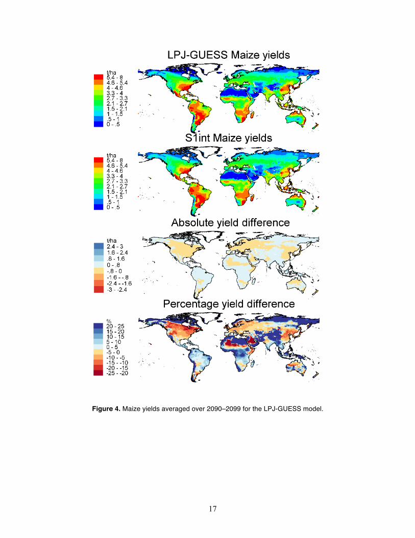
A geographical representation of predicted yields is provided in Figures 3 to 7. The first map in each figure represents, for a particular GGCM, maize yields for each grid cell averaged over the period 2090–2099. The second map shows yields estimated using the S1int specification. For all GGCMs, the statistical model is able to reproduce the spatial distribution of yields reasonably accurately. Both models predict that yields will be the highest in the eastern part of the US, Europe, and China. The LPJ-GUESS and LPJmL models, and associated statistical models, also identify high yield areas in South America. In dry and hot regions, such as the Saharan belt, the Middle East and central Australia, and in the Arctic Circle, maize yields are extremely low.

To further identify differences between projections from the two types of models, the third and fourth maps in Figures 3 to 7 display, respectively, absolute and percentage differences in yields estimated by each GGCM and the corresponding S1int statistical model. These graphs reveal that yield differences are fairly small in absolute terms (between + and -0.8t/ha) for the LPJ-GUESS model. In percentage terms, the maps show large over-predictions from the statistical model in low yield areas, but these are relative to small base values. In areas of high productivity, percentage differences are lower (less than 10% error) especially in the southern parts of America and Africa. For the LPJmL model, the S1int specification underpredicts yields in the Canadian belt. In percentage terms, differences exceeding 20% are predicted globally, but areas of agreement are observed in the most productive regions of Eastern US, South America, and China. For the GEPIC model, the S1int specification moderately under- or overpredicts absolute yields in the western part of the US, but predicts yields in the rest of the globe reasonably accurately. For the pDSSAT model, the spatial distribution of crop yields in absolute terms is represented reasonably well by estimates from the statistical model, with a tendency for the statistical model to over-estimate yields mostly over low-yield areas such as the Sahara, Middle East and central Australia. The largest differences in predicted yields occur when estimating yields for the PEGASUS model. Differences in yield predictions range from -2.8t/ha and +2.8t/ha and some percentage differences are greater than 20%. These differences are also reflected by the relatively high RMSEs associated with the S1int specification for the PEGASUS model (see Table 3).

15

Figure 2. Average maize yield projections from GGCMs and statistical models under the S1int specification.

Note: Shaded areas represents the ‘historical’ period.

16

Figure 3. Maize yields averaged over 2090–2099 for the GEPIC model.

17

Figure 4. Maize yields averaged over 2090–2099 for the LPJ-GUESS model.

18

Figure 5. Maize yields averaged over 2090–2099 for the LPJmL model.

19

Figure 6. Maize yields averaged over 2090–2099 for the pDSSAT model.

20

Figure 7. Maize yields averaged over 2090–2099 for the PEGASUS model.

21

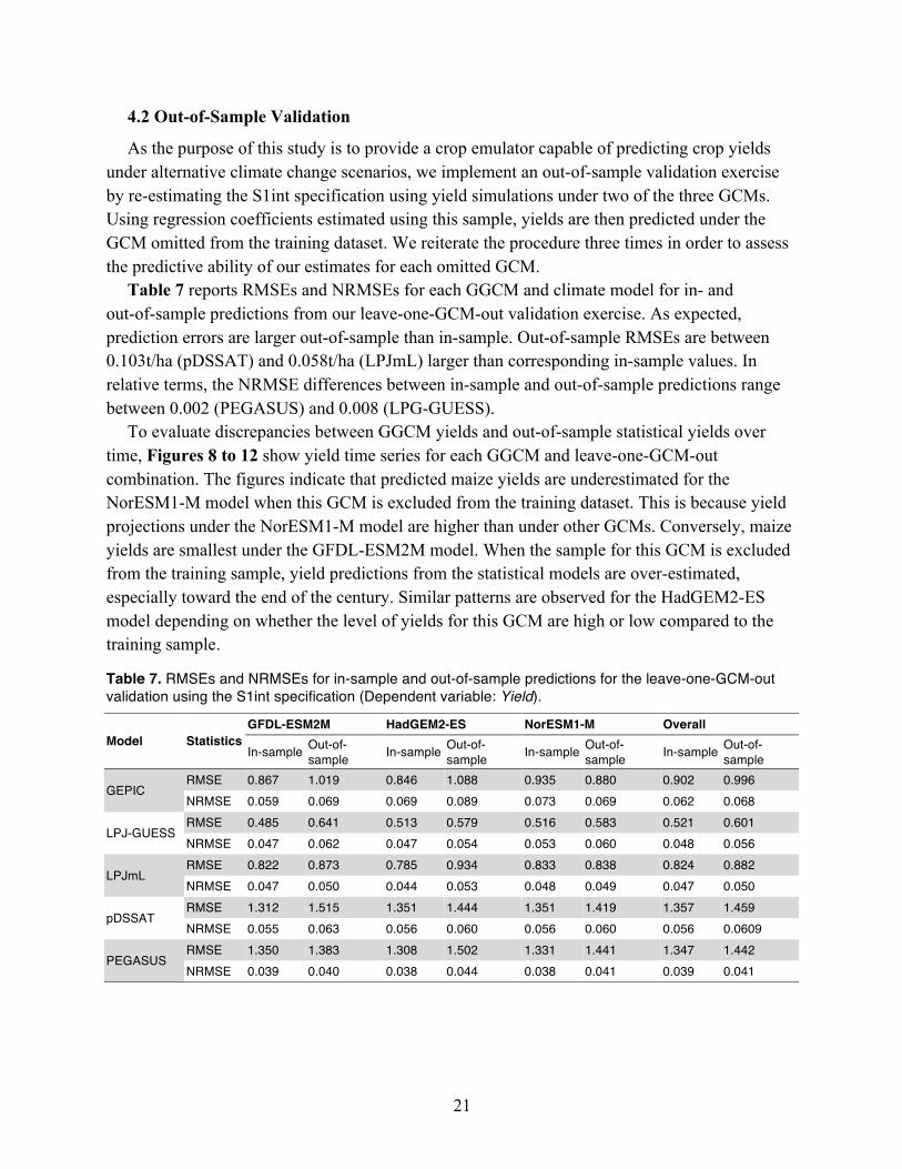
4.2 Out-of-Sample Validation

As the purpose of this study is to provide a crop emulator capable of predicting crop yields under alternative climate change scenarios, we implement an out-of-sample validation exercise by re-estimating the S1int specification using yield simulations under two of the three GCMs. Using regression coefficients estimated using this sample, yields are then predicted under the GCM omitted from the training dataset. We reiterate the procedure three times in order to assess the predictive ability of our estimates for each omitted GCM.

Table 7 reports RMSEs and NRMSEs for each GGCM and climate model for in- and out-of-sample predictions from our leave-one-GCM-out validation exercise. As expected, prediction errors are larger out-of-sample than in-sample. Out-of-sample RMSEs are between 0.103t/ha (pDSSAT) and 0.058t/ha (LPJmL) larger than corresponding in-sample values. In relative terms, the NRMSE differences between in-sample and out-of-sample predictions range between 0.002 (PEGASUS) and 0.008 (LPG-GUESS).

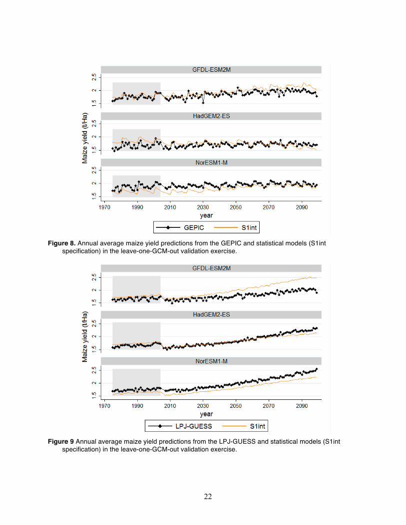
To evaluate discrepancies between GGCM yields and out-of-sample statistical yields over time, Figures 8 to 12 show yield time series for each GGCM and leave-one-GCM-out combination. The figures indicate that predicted maize yields are underestimated for the NorESM1-M model when this GCM is excluded from the training dataset. This is because yield projections under the NorESM1-M model are higher than under other GCMs. Conversely, maize yields are smallest under the GFDL-ESM2M model. When the sample for this GCM is excluded from the training sample, yield predictions from the statistical models are over-estimated, especially toward the end of the century. Similar patterns are observed for the HadGEM2-ES model depending on whether the level of yields for this GCM are high or low compared to the training sample.

Table 7. RMSEs and NRMSEs for in-sample and out-of-sample predictions for the leave-one-GCM-out validation using the S1int specification (Dependent variable: Yield).

Model Statistics GFDL-ESM2M HadGEM2-ES NorESM1-M Overall

In-sample Out-of-sample In-sample Out-of-

sample In-sample Out-of-sample In-sample Out-of-

sample

GEPIC RMSE 0.867 1.019 0.846 1.088 0.935 0.880 0.902 0.996 NRMSE 0.059 0.069 0.069 0.089 0.073 0.069 0.062 0.068

LPJ-GUESS RMSE 0.485 0.641 0.513 0.579 0.516 0.583 0.521 0.601 NRMSE 0.047 0.062 0.047 0.054 0.053 0.060 0.048 0.056

LPJmL RMSE 0.822 0.873 0.785 0.934 0.833 0.838 0.824 0.882 NRMSE 0.047 0.050 0.044 0.053 0.048 0.049 0.047 0.050

pDSSAT RMSE 1.312 1.515 1.351 1.444 1.351 1.419 1.357 1.459 NRMSE 0.055 0.063 0.056 0.060 0.056 0.060 0.056 0.0609

PEGASUS RMSE 1.350 1.383 1.308 1.502 1.331 1.441 1.347 1.442 NRMSE 0.039 0.040 0.038 0.044 0.038 0.041 0.039 0.041

22

Figure 8. Annual average maize yield predictions from the GEPIC and statistical models (S1int

specification) in the leave-one-GCM-out validation exercise.

Figure 9 Annual average maize yield predictions from the LPJ-GUESS and statistical models (S1int

specification) in the leave-one-GCM-out validation exercise.

23

Figure 10. Annual average maize yield predictions from the LPJmL and statistical models (S1int specification) in the leave-one-GCM-out validation exercise.

Figure 11. Annual average maize yield predictions from the pDSSAT and statistical models (S1int specification) in the leave-one-GCM-out validation exercise.

24

Figure 12. Annual average maize yield predictions from the PEGASUS and statistical models (S1int specification) in the leave-one-GCM-out validation exercise.

These results show that it is important to consider the largest ensemble of climate change scenarios possible in order to capture the response function with the best out-of-sample predictive capacity. As the full sample was designed to encompass the extremes ranges of climate change currently being projected, statistical models estimated using this sample are therefore expected to provide reasonable predictions of crop yields even under plausible alternative climate change scenarios.

5. ROBUSTNESS CHECKS

To further assess the appropriateness of the statistical models estimated in Section 3, weimplement a series of robustness tests. Specifically, we separately estimate the S1int specification when the dependent variable is log-transformed, under alternative definitions of the growing season, and when it is estimated separately for sub-global samples.

5.1 Dependent Variable Transformation

For dependent variables characterized by non-negative values and a positively skewed distribution, as is the case with our data, a common estimation strategy consists of regressing the explanatory factors on a log-transformed dependent variable. To test this estimation strategy, and to contend with zero values, we consider the log(Yield+1) as our new dependent variable for the S1int specification. The regression results for each specification of the log-linear model (see Appendix A) show coefficient signs and significance levels very similar to those for the regression in levels.

25

To allow comparison between the log-linear and linear models, we convert the predicted log yields to levels following Wooldridge (2009) and re-estimate the R2 and NRMSE using these values. As indicated by the values for these statistics in Table 8, the log-linear functional form (S1int-log) does not improve the ability of the statistical model to fit the GEPIC, LPJ-GUESS and pDSSAT models. For the LPJmL and PEGASUS models, there are small improvements in model performance from the log-transformation. As log-linear models are more complicated to use for out-of-sample predictions of crop yields than those in levels, and the improvement in model performance is questionable, we prefer the linear functional form to emulate maize yield from GGCMs.

Table 8. Goodness-of-fit measures for the S1int-log (dependent variable: log(Yield+1)) and the S1int specifications (dependent variable: Yield).

Model Statistics S1int-log S1int

GEPIC R2 0.780 0.781 NRMSE 0.062 0.062

LPJ-GUESS R2 0.898 0.903 NRMSE 0.049 0.048

LPJmL R2 0.795 0.791 NRMSE 0.046 0.047

pDSSAT R2 0.702 0.727 NRMSE 0.059 0.056

PEGASUS R2 0.742 0.734 NRMSE 0.038 0.039

5.2 Growing Seasons

In the base specifications, for simplicity, we considered the effect of weather during summer months. However, crop growing seasons vary by grid cell and, as shown in Table 2, can span a wide range of months at the global level. To investigate the benefits of representing growing seasons more precisely, we estimate specification S1int using monthly weather data for the actual growing season for each GGCM. We label this specification S1int-GS. As growing season lengths differ between the Northern and Southern Hemispheres for some GGCMs, we estimate separate regressions for each Hemisphere. For example, specifications for the pDSSAT model considers weather variables for four months (May, June, July and August) in the Northern Hemisphere, and three months (October, November, and December) in the Southern Hemisphere. For the pDSSAT model, growing season information is only available for the HadGEM2-ES climate model, so data for other climate models is not included in the growing-season specific estimates for this model.

Detailed regression results (see Appendix A) show that some weather coefficients are not significant for some months (e.g., T_mean for February and March for the GEPIC model in the Southern Hemisphere). Goodness of fit measures for these regressions are presented in Table 9 and show that the R̄2 and NRMSE values are generally more favorable for the Northern Hemisphere regressions than for the Southern Hemisphere. The overall R̄2, calculated by

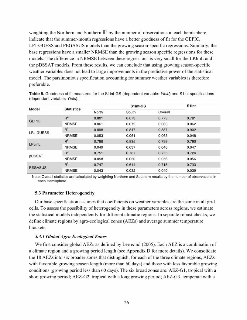
26

weighting the Northern and Southern R̄2 by the number of observations in each hemisphere, indicate that the summer-month regressions have a better goodness of fit for the GEPIC, LPJ-GUESS and PEGASUS models than the growing season-specific regressions. Similarly, the base regressions have a smaller NRMSE than the growing season specific regressions for these models. The difference in NRMSE between these regressions is very small for the LPJmL and the pDSSAT models. From these results, we can conclude that using growing season-specific weather variables does not lead to large improvements in the predictive power of the statistical model. The parsimonious specification accounting for summer weather variables is therefore preferable.

Table 9. Goodness of fit measures for the S1int-GS (dependent variable: Yield) and S1int specifications (dependent variable: Yield).

Model Statistics S1int-GS S1int

North South Overall

GEPIC R2 0.801 0.673 0.773 0.781 NRMSE 0.061 0.072 0.063 0.062

LPJ-GUESS R2 0.898 0.847 0.887 0.902 NRMSE 0.053 0.061 0.063 0.048

LPJmL R2 0.788 0.835 0.799 0.790 NRMSE 0.049 0.037 0.046 0.047

pDSSAT R2 0.751 0.767 0.755 0.726 NRMSE 0.058 0.050 0.056 0.056

PEGASUS R2 0.747 0.614 0.715 0.733 NRMSE 0.043 0.032 0.040 0.039

Note: Overall statistics are calculated by weighting Northern and Southern results by the number of observations in each Hemisphere.

5.3 Parameter Heterogeneity

Our base specification assumes that coefficients on weather variables are the same in all grid cells. To assess the possibility of heterogeneity in these parameters across regions, we estimate the statistical models independently for different climatic regions. In separate robust checks, we define climate regions by agro-ecological zones (AEZs) and average summer temperature brackets.

5.3.1 Global Agro-Ecological Zones We first consider global AEZs as defined by Lee et al. (2005). Each AEZ is a combination of

a climate region and a growing period length (see Appendix D for more details). We consolidate the 18 AEZs into six broader zones that distinguish, for each of the three climate regions, AEZs with favorable growing season length (more than 60 days) and those with less favorable growing conditions (growing period less than 60 days). The six broad zones are: AEZ-G1, tropical with a short growing period; AEZ-G2, tropical with a long growing period; AEZ-G3, temperate with a

27

short growing period; AEZ-G4, temperate with a long growing period; AEZ-G5, boreal with a short growing period; and AEZ-G6, boreal with a long growing period.

Goodness of fit statistics for specification S1int applied to each broad AEZ group (S1int-AEZ) are reported in Table 10 (see Appendix A for detailed regression results). The R̄2 and NRMSE indicate that, in general, the statistical model fits that the data best for the AEZ-G4 and AEZ-G5 subsamples. Overall, the average R̄2 is smaller for the AEZ group regressions than for the global regressions for all models. The average NRMSE is larger for the AEZ group regressions than for the global regressions, but only for the GEPIC, LPJ-GUESS, and pDSSAT models. These results indicate that there are only small differences in performance for the AEZ and global models. Also, the fact that the AEZ groups do not change over time as climate changes is a concern in using this subsampling strategy.

Table 10. Goodness-of-fit measures for S1int-AEZ (dependent variable: Yield) and S1int specifications (dependent variable: Yield). Model Statistics S1int-AEZ S1int

AEZ-G1 AEZ-G2 AEZ-G3 AEZ-G4 AEZ-G5 AEZ-G6 Overall

GEPIC R2 0.727 0.717 0.693 0.716 0.724 0.796 0.724 0.781 NRMSE 0.070 0.052 0.074 0.102 0.042 0.060 0.065 0.062

LPJ-GUESS R2 0.874 0.806 0.863 0.850 0.808 0.827 0.834 0.902 NRMSE 0.071 0.046 0.056 0.056 0.039 0.048 0.051 0.048

LPJmL R2 0.815 0.897 0.775 0.757 0.595 0.677 0.752 0.790 NRMSE 0.032 0.021 0.036 0.062 0.047 0.067 0.043 0.047

pDSSAT R2 0.561 0.664 0.658 0.703 0.613 0.665 0.659 0.726 NRMSE 0.063 0.063 0.062 0.065 0.068 0.071 0.065 0.056

PEGASUS R2 0.728 0.813 0.713 0.671 0.693 0.683 0.724 0.733 NRMSE 0.015 0.016 0.050 0.057 0.036 0.040 0.038 0.039

Note: Overall statistics are calculated by weighting results for each AEZ group by the number of observations in each group.

5.3.2 Average Summer Temperature Brackets We also consider estimating the statistical model for grid cells grouped by average summer

temperatures, which avoids issues associated with AEZs’ inertia to climate change. We divide the sample into eight average summer temperature brackets in 5°C increments, except that the lowest bracket captures all temperatures below 5°C and the highest bracket includes all temperatures above 40°C.

Goodness of fit statistics for specification S1int estimated separately for each average summer temperature bracket (S1int-AST) are reported in Table 11 (detailed regression results are provided in Appendix A). For some models, the bins do not contain enough observations (due to the exclusion of grid cells with less than 10 observations) and regression results and statistics are therefore not available. The model fits the data best when the average summer temperature is between 20°C and 25°C (bracket 25) and between 25°C and 30°C (bracket 30). Overall, the average R̄2 is smaller for all models, except the PEGASUS model, using the temperature bins

28

subsamples than for the global sample. For the PEGASUS model, this finding can be explained by the lack of results for bins with very low and high summer temperatures, which are characterized by smaller R̄2 in other models. The NRMSE are also smaller for the global sample than the temperature bracket subsamples for most models. Subsampling by temperature brackets does not appear to provide better estimates for our crop yield statistical model than the global specification.

Table 11. Goodness-of-fit measures for the S1int-AST (dependent variable: Yield) and S1int specifications (dependent variable: Yield).

Model Statistics S1int-AST S1int <5 10 15 20 25 30 35 >40 Overall

GEPIC R2 0.003 0.441 0.768 0.794 0.777 0.783 0.748 0.383 0.743 0.781 NRMSE 0.006 0.094 0.041 0.055 0.080 0.068 0.074 0.074 0.066 0.062

LPJ-GUESS R2 0.968 0.927 0.817 0.806 0.881 0.873 0.899 0.649 0.860 0.902 NRMSE 0.012 0.012 0.029 0.041 0.047 0.053 0.067 0.09 0.046 0.048

LPJmL R2 - -0.004 0.553 0.77 0.846 0.903 0.877 0.645 0.779 0.790 NRMSE - 0.003 0.033 0.055 0.047 0.030 0.031 0.048 0.037 0.047

pDSSAT R2 - 0.255 0.627 0.749 0.785 0.723 0.654 0.655 0.722 0.726 NRMSE - 0.043 0.055 0.054 0.055 0.074 0.060 0.043 0.057 0.056

PEGASUS R2 - - 0.695 0.743 0.787 0.782 0.630 - 0.751 0.733 NRMSE - - 0.047 0.034 0.043 0.034 0.039 - 0.037 0.039

Note: Overall statistics are average statistics weighted by observation; Statistics are not reported for some temperature-GGCM combinations due to lack of data.

6. CONCLUDING REMARKS

The goal of this analysis is to provide a simple simulation tool to allow researchers to predict the impact of climate change on maize yields. To this end, we used an ensemble of crop yield simulations from five GGCMs included in the ISI-MIP Fast Track experiment, which simulate the impact of weather on maize yields under various climate change scenarios. We then estimated a response function for each crop model.

As shown in the ISI-MIP simulations, the different GGCMs do not necessarily agree on the extent of the impact of climate change on crop yields. As none of the models is deemed better than another at projecting future yields, it is important to consider predictions from many models to account for uncertainty in the impact of climate change on crop yields. Consequently, this study provided response function estimates for several crop models.

This study evaluated a large set of weather variables, including temperature and precipitation, non-linear transformations and interactions between temperature and precipitation, and other composites based on these variables. Our results showed that specifications that included temperature and precipitation separately, in quadratic forms and a temperature-precipitation interaction term performed relatively well and specifications that included more complicated composite terms resulted in only small improvements in the ability of the model to predict crop yields.

29

Our validation exercises showed that out-of-sample maize yield predictions are reasonably accurate, especially with respect to long-term trends. The analysis also showed that prediction accuracy was lowered when the training sample excluded yield responses to weather variables outside the range of values used to estimate the model. For this reason, our statically models were estimated using data that encompass the range of plausible changes in temperature and precipitation over the twenty-first century.

In robustness analyses, we considered transforming the dependent variable, more precisely representing the growing season, and estimating the statistical model separately for alternative climatic regions. None of these modifications resulted in significant improvements relative to the parsimonious base specification.

Based on these findings, this study provides simple crop model emulators for five crop models that predict changes in maize yields based on changes in precipitation and simple transformations of these variables. These emulators provide a quick and easy way for researchers to estimate changes in maize yields under user-defined changes in climate and will be useful for climate change impact assessments and other purposes.

Acknowledgments The authors thank Niven Winchester for helpful comments and suggestions, and Joshua

Elliott and Christian Folberth for kindly providing further details regarding, respectively, the GEPIC and pDSSAT model. The MIT Joint Program on the Science and Policy of Global Change is funded through a consortium of industrial sponsors and Federal grants.

7. REFERENCESAlexandrov, V.A. and G. Hoogenboom, 2000: Vulnerability and adaptation assessments of

agricultural crops under climate change in the Southeastern USA. Theor. Appl. Climatol., 67(1-2): 45-63.

Allen, R.G., L.S. Pereira, D. Raes and M. Smith, 1998: Crop evapotranspiration - Guidelines for computing crop water requirements. Food and Agricultural Organization, Rome.

Asseng, S., S. Millroy, S. Bassu and M. Abi Saab, 2012: Herbaceous crops (3.4). Food and Agriculture Organization of the United Nations, Rome, Italy.

Basso, B., D. Cammarano and E. Carfagna, 2013: Review of Crop Yield Forecasting Methods and Early Warning Systems. Food and Agriculture Organization of the United Nations.

Bassu, S., N. Brisson, J.-L. Durand, K. Boote, J. Lizaso, J.W. Jones, C. Rosenzweig, A.C. Ruane, M. Adam, C. Baron, B. Basso, C. Biernath, H. Boogaard, S. Conijn, M. Corbeels, D. Deryng, G. De Sanctis, S. Gayler, P. Grassini, J. Hatfield, S. Hoek, C. Izaurralde, R. Jongschaap, A.R. Kemanian, K.C. Kersebaum, S.-H. Kim, N.S. Kumar, D. Makowski, C. Müller, C. Nendel, E. Priesack, M.V. Pravia, F. Sau, I. Shcherbak, F. Tao, E. Teixeira, D. Timlin and K. Waha, 2014: How Do Various Maize Crop Models Vary in Their Responses to Climate Change Factors? Global Change Biology 20(7): 2301-20.

Blanc, É., 2012: The impact of climate change on crop yields in Sub-Saharan Africa. American Journal of Climate Change 1(1): 1-13.

30

Blanc, E. and E. Strobl, 2013: Is Small Better? A Comparison of the Effect of Large and Small Dams on Cropland Productivity in South Africa. The World Bank Economic Review.

Blanc, E. and E. Strobl, 2014: Water availability and crop growth at the crop plot level in South Africa modelled from satellite imagery. Journal of Agricultural Science, FirstView: 1-16.

Bondeau, A., P.C. Smith, S. Zaehle, S. Schaphoff, W. Lucht, W. Cramer, D. Gerten, H. Lotze-Campen, C. Müller, M. Reichstein and B. Smith, 2007: Modelling the Role of Agriculture for the 20th Century Global Terrestrial Carbon Balance. Global Change Biology 13(3): 679-706.

Carter, C. and B. Zhang, 1998: Weather factor and variability in China's grain supply. Journal of Comparative Economics 26: 529-543.

Corobov, R., 2002: Estimations of climate change impacts on crop production in the Republic of Moldova. Geojournal 57: 195-202.

Cuculeanu, V., A. Marica and C. Simota, 1999: Climate change impact on agricultural crops and adaptation options in Romania. Climate Research, 153-160.

Deryng, D., W.J. Sacks, C.C. Barford and N. Ramankutty, 2011: Simulating the effects of climate and agricultural management practices on global crop yield. Global Biogeochem. Cycles 25(2): GB2006.

Dixon, B.L., S.E. Hollinger, P. Garcia and V. Tirupattur, 1994: Estimating Corn Yield Response Models to Predict Impacts of Climate Change. Journal of Agricultural and Resource Economics 19(1): 58-68.

Elliott, J., M. Glotter, N. Best, D. Kelly, M. Wilde and I. Foster, 2013: The Parallel System for Integrating Impact Models and Sectors (Psims). Paper presented at the Conference on Extreme Science and Engineering Discovery Environment: Gateway to Discovery 2013 (XSEDE ’13).

Hargreaves, G.H. and Z.A. Samani, 1985: Reference crop evapotranspiration from temperature. Appl. Eng. Agric. (1): 96-99.

Hempel, S., K. Frieler, L. Warszawski, J. Schewe, and F. Piontek, 2013: A trend-preserving bias correction &ndash; the ISI-MIP approach. Earth Syst. Dyn. 4(2): 219-236.

Holzkämper, A., P. Calanca and J. Fuhrer, 2012: Statistical crop models: predicting the effects of temperature and precipitation changes. Climate Research 51(1): 11-21.

Izaurralde, R.C.C., J.R. Williams, W.B. Mcgill, N.J. Rosenberg and M.C.Q. Jakas, 2006: Simulating soil C dynamics with EPIC: Model description and testing against long-term data. Ecol. Modell. 192(3-4): 362-384.

Jones, J., G. Hoogenboom, C. Porter, K. Boote, W. Batchelor, L. Hunt and J. Ritchie, 2003: The Dssat Cropping System Model. European Journal of Agronomy 18(3-4): 235-65.

Lee, H.-L., T. Hertel, B. Sohngen and N. Ramankutty, 2005: Towards An Integrated Land Use Data Base for Assessing the Potential for Greenhouse Gas Mitigation.

Lindeskog, M., A. Arneth, A. Bondeau, K. Waha, J. Seaquist, S. Olin, and B. Smith, 2013: Implications of Accounting for Land Use in Simulations of Ecosystem Services and Carbon Cycling in Africa. Earth System Dynamics Discussions 4, 235-78.

Liu, J., J.R. Williams, A.J.B. Zehnder and H. Yang, 2007: GEPIC – modelling wheat yield and crop water productivity with high resolution on a global scale. Agric. Syst. 94(2): 478-493.

31

Lobell, D. and C. Field, 2007: Global scale climate-crop yield relationships and the impacts of recent warming. Environ. Res. Lett. 2(1): 1-7.

Lobell, D.B. and G.P. Asner, 2003: Climate and Management Contributions to Recent Trends in U.S. Agricultural Yields. Science 299(5609): 1032.

Lobell, D.B., M. Banziger, C. Magorokosho and B. Vivek, 2011: Nonlinear heat effects on African maize as evidenced by historical yield trials. Nature Climate Change 1(1): 42-45.

Lobell, D.B. and M.B. Burke, 2010: On the use of statistical models to predict crop yield responses to climate change. Agric. For. Meteorol. 150(11): 1443-1452.

Lobell, D.B., M.J. Roberts, W. Schlenker, N. Braun, B.B. Little, R.M. Rejesus and G.L. Hammer, 2014: Greater Sensitivity to Drought Accompanies Maize Yield Increase in the U.S. Midwest. Science 344(6183): 516-19.

Mearns, L.O., T. Mavromatis, E. Tsvetsinskaya, C. Hays and W. Easterling, 1999: Comparative responses of EPIC and CERES crop models to high and low spatial resolution climate change scenarios. Journal of Geophysical Research: Atmospheres 104(D6): 6623-6646.

Nicholls, N., 1997: Increased Australian wheat yield due to recent climate trends. Nature 387: 484-485.

Oyebamiji, O.K., N.R. Edwards, P.B. Holden, P.H. Garthwaite, S. Schaphoff and D. Gerten, 2015: Emulating global climate change impacts on crop yields. Statistical Modelling, in press.

Riahi, K., A. Gruebler and N. Nakicenovic, 2007: Scenarios of long-term socio-economic and environmental development under climate stabilization. Technol. Forecasting Social Change 74(7): 887-935.

Rosenzweig, C., J. Elliott, D. Deryng, A.C. Ruane, C. Müller, A. Arneth, K. J. Boote, C. Folberth, M. Glotter, N. Khabarov, K. Neumann, F. Piontek, T.A.M. Pugh, E. Schmid, E. Stehfest, H. Yang and J.W. Jones, 2014: Assessing agricultural risks of climate change in the 21st century in a global gridded crop model intercomparison. Proceedings of the National Academy of Sciences 111(9): 3268-3273.

Rosenzweig, C., J.W. Jones, J.L. Hatfield, A.C. Ruane, K.J. Boote, P. Thorburn, J.M. Antle, G.C. Nelson, C. Porter, S. Janssen, S. Asseng, B. Basso, F. Ewert, D. Wallach, G. Baigorria and J.M. Winter, 2013: The Agricultural Model Intercomparison and Improvement Project (AgMIP): Protocols and pilot studies. Agric. For. Meteorol. 170(0): 166-182.

Schlenker, W. and D.B. Lobell, 2010: Robust negative impacts of climate change on African agriculture. Environ. Res. Lett. 5: 1-8.

Smith, B., I.C. Prentice and M.T. Sykes, 2001: Representation of vegetation dynamics in the modelling of terrestrial ecosystems: comparing two contrasting approaches within European climate space. Global Ecol. Biogeogr. 10(6): 621-637.

StataCorp, 2011: Stata Statistical Software: Release 12. StataCorp LP, College Station, TX. Strobl, E. and R.O. Strobl, 2010: The distributional impact of large dams: Evidence from

cropland productivity in Africa. Journal of Development Economics 96(2): 1-19. Taylor, K.E., R.J. Stouffer and G.A. Meehl, 2012: An Overview of CMIP5 and the experiment

design. Bull. Am. Meteorol. Soc. 93: 485-498.

32

Waha, K., L.G.J. van Bussel, C. Müller and A. Bondeau, 2012: Climate-driven simulation of global crop sowing dates. Global Ecol. Biogeogr. 21(2): 247-259.

Warszawski, L., K. Frieler, V. Huber, F. Piontek, O. Serdeczny and J. Schewe, 2014: The Inter-Sectoral Impact Model Intercomparison Project (ISI-MIP): Project framework. Proceedings of the National Academy of Sciences 111(9): 3228-3232.

Williams, J., 1995: Chapter 25. The EPIC, Computer Models of Watershed Hydrology. Water Resources Publications, Littleton, CO, pp. 909-1000.

Wooldridge, J.M., 2009: Introductory econometrics: a modern approach. Thomson/South-Western, Mason, OH, 890 pp.

You, L., M.W. Rosegrant, S. Wood and D. Sun, 2009: Impact of growing season temperature on wheat productivity in China. Agric. For. Meteorol. 149: 1009-1014.

33

APPENDIX A. REGRESSION RESULTS

See attached Excel file Appendix_A_regression_results.xls composed of the following tables: Table A1. Regression results for all specifications for the GEPIC model (dependent variable: Yield). Table A2. Regression results for all specifications for the LPJ-GUESS model (dependent variable: Yield). Table A3. Regression results for all specifications for the LPJmL model (dependent variable: Yield). Table A5. Regression results for all specifications for the PEGASUS model (dependent variable: Yield). Table A6. Regression results for the S1int-log specifications for all GGCMs (dependent

variable: log(Yield+1)). Table A7. Regression results for the S1int-GS specification for each GGCM and Hemisphere (dependent

variable: Yield). Table A8. Regression results for the S1-AEZ specification for the GEPIC model (dependent

variable: Yield). Table A9. Regression results for the S1-AEZ specification for the LPJ-GUESS model (dependent

variable:Yield). Table A10. Regression results for the S1-AEZ specification for the LPJmL model (dependent

variable: Yield). Table A11. Regression results for the S1-AEZ specification for the pDSSAT model (dependent

variable: Yield). Table A12. Regression results for the S1-AEZ specification for the PEGASUS model (dependent

variable: Yield). Table A13. Regression results for the S1-AST specifications for the GEPIC model (dependent

variable: Yield). Table A14. Regression results for the S1-AST specifications for the LPJ-GUESS model (dependent

variable: Yield). Table A15. Regression results for the S1-AST specifications for the LPJmL model (dependent

variable: Yield). Table A16. Regression results for the S1-AST specifications for the pDSSAT model (dependent

variable: Yield). Table A17. Regression results for the S1-AST specifications for the PEGASUS model (dependent

variable: Yield).

APPENDIX B. FIXED EFFECTS (δ) BY SPECIFICATION AND CROP MODEL

See attached Excel file Appendix_B_ Grid_cells_FE.xls composed of the following tables:

Table B1. Grid cell fixed effect (δ) by specification for the GEPIC model. Table B2. Grid cell fixed effect (δ) by specification for the LPJmL model. Table B3. Grid cell fixed effect (δ) by specification for the LPJ-GUESS model. Table B4. Grid cell fixed effect (δ) by specification for the pDSSAT model. Table B5. Grid cell fixed effect (δ) by specification for the PEGASUS model.

34

APPENDIX C. TEMPERATURE AND PRECIPITATION EFFECT FROM THE S1INT SPECIFICATION

Figure C1. Effect of Tmean and Pr on maize yields for GEPIC model in the S1int specification.

35

Figure C2. Effect of Tmean and Pr on Maize yields for the LPJ-GUESS model in the S1int specification.

36

Figure C3. Effect of Tmean and Pr on maize yields for the LPJmL model in the S1int specification.

37

Figure C4. Effect of Tmean and Pr on maize yields for pDSSAT model in the S1int specification.

38

Figure C5. Effect of Tmean and Pr on maize yields for the PEGASUS model in the S1int specification.

39

APPENDIX D

Figure D1. Map of the 18 global AEZs.

Table D2. Identification of SAGE 18 AEZs by length of the growing period (LGP) and climate zone.

LGP in days Climate Zones

Tropical Temperate Boreal 0-59 AEZ1 AEZ7 AEZ13 60-119 AEZ2 AEZ8 AEZ14 120-179 AEZ3 AEZ9 AEZ15 180-239 AEZ4 AEZ10 AEZ16 240-299 AEZ5 AEZ11 AEZ17 >300 AEZ6 AEZ12 AEZ18

Table D3. AEZ groups based on 18 AEZs.

AEZ groups AEZ Growing Period Climate Zones AEZ-G1 1, 2 Short Growing Period Tropical AEZ-G2 3, 4, 5, 6 Long Growing Period Tropical AEZ-G3 7, 8 Short Growing Period Temperate AEZ-G4 9, 10, 11, 12 Long Growing Period Temperate AEZ-G5 13, 14 Short Growing Period Boreal AEZ-G6 15, 16, 17, 18 Long Growing Period Boreal

REPORT SERIES of the MIT Joint Program on the Science and Policy of Global ChangeFOR THE COMPLETE LIST OF JOINT PROGRAM REPORTS: http://globalchange.mit.edu/pubs/all-reports.php

Contact the Joint Program Office to request a copy. The Report Series is distributed at no charge.

260. Electricity Generation and Emissions Reduction Decisions under Policy Uncertainty: A General Equilibrium Analysis. Morris et al., April 2014

261. An Integrated Assessment of China’s Wind Energy Potential. Zhang et al., April 2014

262. The China-in-Global Energy Model. Qi et al. May 2014

263. Markets versus Regulation: The Efficiency and Distributional Impacts of U.S. Climate Policy Proposals. Rausch and Karplus, May 2014

264. Expectations for a New Climate Agreement. Jacoby and Chen, August 2014

265. Coupling the High Complexity Land Surface Model ACASA to the Mesoscale Model WRF. Xu et al., August 2014

266. The CO2 Content of Consumption Across US Regions: A Multi-Regional Input-Output (MRIO) Approach. Caron et al., August 2014

267. Carbon emissions in China: How far can new efforts bend the curve? Zhang et al., October 2014

268. Characterization of the Solar Power Resource in Europe and Assessing Benefits of Co-Location with Wind Power Installations. Bozonnat and Schlosser, October 2014

269. A Framework for Analysis of the Uncertainty of Socioeconomic Growth and Climate Change on the Risk of Water Stress: a Case Study in Asia. Fant et al., November 2014

270. Interprovincial Migration and the Stringency of Energy Policy in China. Luo et al., November 2014

271. International Trade in Natural Gas: Golden Age of LNG? Du and Paltsev, November 2014

272. Advanced Technologies in Energy-Economy Models for Climate Change Assessment. Morris et al., December 2014

273. The Contribution of Biomass to Emissions Mitigation under a Global Climate Policy. Winchester and Reilly, January 2015

274. Modeling regional transportation demand in China and the impacts of a national carbon constraint. Kishimoto et al., January 2015.

275. The Impact of Advanced Biofuels on Aviation Emissions and Operations in the U.S. Winchester et al., February 2015

276. Specifying Parameters in Computable General Equilibrium Models using Optimal Fingerprint Detection Methods. Koesler, February 2015

277. Renewables Intermittency: Operational Limits and Implications for Long-Term Energy System Models. Delarue and Morris, March 2015

278. The MIT EPPA6 Model: Economic Growth, Energy Use, and Food Consumption. Chen et al., March 2015

279. Emulating maize yields from global gridded crop models using statistical estimates. Blanc and Sultan, March 2015

239. Analysis of U.S. Water Resources under Climate Change. Blanc et al., February 2013

240. Protection of Coastal Infrastructure under Rising Flood Risk. Lickley et al., March 2013

241. Consumption-Based Adjustment of China’s Emissions-Intensity Targets: An Analysis of its Potential Economic Effects. Springmann et al., March 2013

242. The Energy and CO2 Emissions Impact of Renewable Energy Development in China. Zhang et al., April 2013

243. Integrated Economic and Climate Projections for Impact Assessment. Paltsev et al., May 2013

244. A Framework for Modeling Uncertainty in Regional Climate Change. Monier et al., May 2013

245. Climate Change Impacts on Extreme Events in the United States: An Uncertainty Analysis. Monier and Gao, May 2013

246. Probabilistic Projections of 21st Century Climate Change over Northern Eurasia. Monier et al., July 2013

247. What GHG Concentration Targets are Reachable in this Century? Paltsev et al., July 2013

248. The Energy and Economic Impacts of Expanding International Emissions Trading. Qi et al., August 2013

249. Limited Sectoral Trading between the EU ETS and China. Gavard et al., August 2013

250. The Association of Large-Scale Climate Variability and Teleconnections on Wind Resource over Europe and its Intermittency. Kriesche and Schlosser, September 2013

251. Regulatory Control of Vehicle and Power Plant Emissions: How Effective and at What Cost? Paltsev et al., October 2013

252. Synergy between Pollution and Carbon Emissions Control: Comparing China and the U.S. Nam et al., October 2013

253. An Analogue Approach to Identify Extreme Precipitation Events: Evaluation and Application to CMIP5 Climate Models in the United States. Gao et al. November 2013

254. The Future of Global Water Stress: An Integrated Assessment. Schlosser et al., January 2014

255. The Mercury Game: Evaluating a Negotiation Simulation that Teaches Students about Science–Policy Interactions. Stokes and Selin, January 2014

256. The Potential Wind Power Resource in Australia: A New Perspective. Hallgren et al., February 2014

257. Equity and Emissions Trading in China. Zhang et al., February 2014

258. Characterization of the Wind Power Resource in Europe and its Intermittency. Cosseron et al., March 2014

259. A Self-Consistent Method to Assess Air Quality Co-Benefits from US Climate Policies. Saari et al., April 2014