Empirical Study BlockPlacement by Cluster...

VLSI DESIGN1999, Vol. 10, No. 1, pp. 71-86Reprints available directly from the publisherPhotocopying permitted by license only

(C) 1999 OPA (Overseas Publishers Association) N.V.Published by license under

the Gordon and Breach SciencePublishers imprint.

Printed in Malaysia.

Empirical Study of Block Placementby Cluster Refinement

JIN XU a, PEI-NING GUO b and CHUNG-KUAN CHENGb’*

Cadence Design Systems, Inc., 555 River Oaks Parkway, San Jose, CA 95134,"b Department of Computer Science and Engineering, University of California, San Diego, La Jolla, CA 92093-0114

(Received 7 September 1998; In finalform 20 November 1998)

In this paper we propose an efficient cluster refinement approach for macro-cell place-ment. The algorithm selects a cluster ofblocks dynamically, and finds an optimal solutionfor all the blocks in the cluster simultaneously. This is different from previous zone re-finement approach which optimizes the allocation of one single block in each operation.Experimental results on the MCNC benchmark circuits show that the approach achievesexcellent area utilization while minimizing the wire length at the same time.

Keywords." VLSI, layout, physical design, placement

1. INTRODUCTION

Placement of blocks on a 2D surface is one criticalprocess in VLSI layout design. The major objec-tives are chip area and wire length minimization.Since the number of possible placements increasesexplosively with the number of blocks, even sub-sets of the problem have been shown to be NP-complete or NP-hard [13].Onodera et al. [13] presents a building block

placement approach which employs a branch-and-bound strategy to search for an optimal solutionwithin the whole solution space of size 2n(n+2>. Themaximum number of blocks which can be placed

in a reasonable amount of CPU time is aroundsix. Large problems are decomposed to reduce thenumber of blocks below the manageable limit,and a placement is constructed hierarchically in abottom-up manner.

H. Murata et al. [11] introduces a P-admissiblesolution space of size (n!)2 8n, where n is the totalnumber of blocks, and applies a simulated anneal-ing method to search for a good solution.

Shin et al. [15] applies zone refinement techniquein IC layout compaction. Blocks are peeled off rowby row from the precompacted layout, movedacross an open zone, and reassembled at the otherend of the zone in a denser configuration. They

*Corresponding author. Tel." (619)534-6184, Fax: (619)534-7029, e-mail: [email protected]

71

72 J. XU et al.

sweep across the zone to optimize the allocation ofone single block in each operation.Note that the above approaches can be applied

to general structures. For slicing structure, Yama-nouchi et al. [18] proposes a partial clustering andmodule restructuring algorithm.

In this paper, we present a new cluster refine-ment approach, which consists of the followingthree parts:

(1) sequential cluster selection which reduces thecomplexity of the problem to a manageabledegree;

(2) cluster optimization which employs an efficientbranch-and-bound strategy to search for anoptimal solution for all the blocks in thecluster;

(3) adaptive cluster overlapping which exploreslarger solution space to achieve better results.

To demonstrate the efficiency of the algorithm,we apply our algorithm to the MCNC benchmarkcircuits. Experimental results show that the algo-rithm obtains excellent area utilization while mini-mizing the wire length at the same time.The following sections in this paper are orga-

nized as follows. We formulate the problem inSection 2. Section 3 describes the details of thealgorithm. Then the complexity analysis andexperimental results are given in Section 4 andSection 5 respectively. Finally, Section 6 presentsconcluding remarks.

2. PROBLEM DESCRIPTION

Inputs of the placement problem are

a set of blocks with fixed geometries and fixedpin positions.a set of nets specifying the interconnectionsbetween pins of the blocks.a set of pads (external pins) with fixed positions.a set of user constraints, e.g., block position/orientation, critical nets, if any Given the inputspecifications, the objective of the problem is to

find the positions and orientations of eachblock, so that the chip area and wire length be-tween blocks are minimized while satisfying allthe given constraints.

Since it is impractical to calculate the exact wirelength at placement stage where detailed routinghas not yet been carried out, we estimate the lengthof each net as one-half of the perimeter of theminimum bounding box of the net.The objective function, which measures the

quality of the resulting placement, can be ex-pressed as follows,

E C1 ChipArea + C2 x WireLength

where C1 and C2 are the constant weights for chiparea and wire length respectively.

3. CLUSTER REFINEMENT ALGORITHM

Cluster refinement algorithm intends to improveover traditional zone refinement algorithm bygiving more flexibility on cluster selection. Withthe capabilities of cluster optimization and over-lapping, cluster refinement algorithm provides abetter approach for block placement. The detaildescription of cluster refinement algorithm is givenas follows.

3.1. Overall Algorithm

Zone refinement is a technique used in the purifica-tion process of crystal ingots. It provides a generalframework for reducing the total number of blocksto the degree which can be handled at one time.However, the traditional zone refinement algo-

rithm [15] probably cannot find the optimal solu-tion due to the predetermined order of the blocks.Figure illustrates an example. If block A isplaced in its best position, which is also the bestposition for block B. It is impossible for block Bto be placed in its best position if we place blockA first. Therefore, the better solution is preventedin this case.

PHYSICAL DESIGN 73

(a) (b)

FIGURE Illustration of placement by different orders. (a) Afirst, (b) B first.

The major contribution of our work is thatwe select a cluster of blocks dynamically, employa branch-and-bound strategy to find an optimalsolution for all blocks, then move the blocks in thecluster simultaneously.

Figure 2 shows the situation when cluster refine-ment is in progress. A placement consists of tworegions ofblocks, separated by a zone called a ’gap’.The lower bound ofthe top region forms the ’ceiling’profile, while the upper bound of the bottom regionforms the ’floor’ profile, as illustrated by the boldlines. The ’gap’ profile is obtained by ’deducting’ theceiling from the floor profile.When cluster refinement starts, all blocks are in

the ceiling region, while the floor region and thecluster are totally empty. First a cluster of blocksis selected by the cluster selection algorithm, andis ’peeled off’ from the ceiling. Then the clusteroptimization algorithm is applied to the cluster,and the cluster is placed onto the floor based onthe results obtained. A new cluster is obtained bythe cluster overlapping algorithm and the cluster

ceiling

oor

FIGURE 2 Cluster refinement in progress.

optimization algorithm is applied to the newcluster. The algorithm loops until the ceiling isempty.

Figure 3 shows the outline of the algorithm. Thealgorithm improves an initial placement alongone direction, alternates the optimizing directionand begins the next iteration. It may iterate manytimes until no improvement is achieved, or a givennumber of iterations is reached.

3.2. Cluster Selection

Our cluster selection algorithm is based on theconstraint graphs [15]. It selects a cluster adap-tively and sequentially, according to the currentpartial placement. We first give the definitionof neighbors, then present the cluster selectionalgorithm.

DEFINITION TWO blocks are neighbors if they areadjacent to each other in either the horizontal orthe vertical constraint graph.

Therefore, two blocks are horizontal neighbors ifthey are adjacent in horizontal constraint graph,vertical neighbors if adjacent in vertical constraintgraph.For example, in Figure 4(a), the neighbors of

block are block 2(right), block 3(above) andblock 4(above), based on the constraint graphsshown in Figure 4(b), where block 2 is its horizon-tal neighbor, while blocks 3 and 4 are its verticalneighbors.The algorithm identifies the block which dom-

inates the minimum gap distance to be the ’critical’block, then build up a cluster of size k with thisblock and its k-1 neighbors. Figure 5 shows theoutline of the cluster selection algorithm.

In Figure 4(a), block is identified first and acluster of size 4 is built up with it and its threeneighbors, blocks 2, 3 and 4.Note that the cluster size k here is actually the

upper bound. The algorithm can adopt flexiblecluster size, depending on the number of neigh-bors of the critical block. For example, in Figure 6,if k 4, but the critical block only has 2

74 J. XU et al.

ClusterRefinement

Select a compaction direction;

for(n:O; n<IterationNumber; n++)

Construct the ceiling;

Initialize the floor;

while(ceiling not empty)

ClusterOverlapping;

Update the ceiling;

ClusterOptimization;

Update the floor;

Alternate the compaction direction;

FIGURE 3 Outline of the algorithm.

ceiling

horizontal constrainl

vertical constraint

@

(a) (b)

FIGURE 4 Cluster selection in progress. (a) Cluster selected (b) Constraint graphs for block 1.

neighbors, block 2 and 3, the cluster obtained willbe of size 3.

3.3. Cluster Optimization

In order to find an optimal solution, we evaluateall of the possible configurations on the selectedcluster. Because the number of possible combina-tions increases exponentially with the number ofblocks in the cluster, we employ a branch-and-

bound technique to explore the solution spaceeffectively.

3.3.1. Branching Operations

We enumerate the state space as a tree whosenodes correspond to partial placements for someblocks in the cluster. The successors of a nodecorrespond to the implementation of the blocks tobe considered next. A path from the root to a leafrepresents a complete placement for the cluster.

PHYSICAL DESIGN 75

ClusterSelection (k)

Identify a critical block u;

Add u to the cluster;

Sort u’s horizontal neighbors in y dimension from low to high;

Sort u’s vertical neighbors in x dimension from right to left;

Append vertical neighbor list to horizontal neighbor list;

repeat until k blocks are selected or u has no neighbors left

Find the first neighbor v;

if v has no vertical neighbors below it

add v to the cluster;

Delete v from u’s neighbor list;

FIGURE 5 Cluster selection algorithm.

ceiling

tloor

horizontal

vertical

(a) (b)

FIGURE 6 Cluster size k as a upper bound. (a) Cluster selected, (b) Constraint.

3.3.2. Order

Suppose k blocks are selected in the cluster andare numbered 1, 2,...,k. To find the best orderof placing the blocks, we try all of their combi-nations, i.e., k! permutations, as shown in therecursive permutation tree in Figure 7.

3.3.3. Rotation

Each block may be specified in any one of eightorientations, i.e., two rotations and four reflec-tions (Fig. 8). We specify one rotation out oftwo foreach block when placing each block, because rota-

tion is closely related to the final chip area. Sincereflection is only directly related to wire length, wetry the four reflections for each block only whenmaking estimates to reduce the total wire length.

(53Pn(1,2 n...

Pn. (2,3 1(1,3 n) Pn_ (1,2 n-1

Pn_2(3,4 n) Pn-2(1,4 n) Pn-2(l,3 n-l)

FIGURE 7 Recursive permutation tree.

76 J. XU et al.

(a) (b)

FIGURE 8 Orientation of a block. (a) Rotation, (b) Reflection.

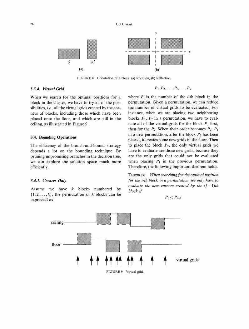
3.3.4. Virtual Grid

When we search for the optimal positions for ablock in the cluster, we have to try all of the pos-sibilities, i.e., all the virtual grids created by the cor-ners of blocks, including those which have beenplaced onto the floor, and which are still in theceiling, as illustrated in Figure 9.

3.4. Bounding Operations

The efficiency of the branch-and-bound strategydepends a lot on the bounding technique. Bypruning unpromising branches in the decision tree,we can explore the solution space much moreefficiently.

3.4.1. Corners Only

Assume we have k blocks numbered by{1,2,...,k}, the permutation of k blocks can beexpressed as

P1,P2,... ,Pi,. ,Pk

where Pi is the number of the i-th block in thepermutation. Given a permutation, we can reducethe number of virtual grids to be evaluated. Forinstance, when we are placing two neighboringblocks P1, P2 in a permutation, we have to eval-uate all of the virtual grids for the block PI first,then, for the P2. When their order becomes P2, P1in a new permutation, after the block P2 has beenplaced, it creates some new grids in the floor. Thento place the block P1, the only virtual grids wehave to evaluate are those new grids, because theyare the only grids that could not be evaluatedwhen placing P1 in the previous permutation.Therefore, the following important theorem holds.

THEOREM When searchingfor the optimalpositionfor the i-th block in a permutation, we only have to

evaluate the new corners created by the (i-1)thblock if

Pi < Pi-1

ceiling

floor

FIGURE 9 Virtual grid.

virtual grids

PHYSICAL DESIGN 77

In general, we have to search for all of thevirtual grids to place a block. The theorem abovesuggests that we only need to evaluate thosevirtual grids in the range from the leftmost to therightmost position of the previous block (Fig. 10),because all other possibilities have been coveredwhen placing the blocks by other permutations.This greatly reduces the search space and let thealgorithm prune unpromising branches and reachthe optimal solution much more efficiently.For example, if Pi < Pi-1, after Pi-1 has been

placed as shown in the figure above, to place Pi,the number of virtual grids we have to evaluate isonly two (Fig. 10).

3.4.2. Lower[Upper Bound

We first place each block in the cluster at itsoriginal x-position, and calculate the cost func-tions and record their values and the x-positions asthe current best knoWn solution. Those values,along with the constraints given, provide lower/upper bounds for the placements obtained in thesearch process later. The cost functions used in thispaper are as follows: gap distance, chip width, chiplength, dead space created, wire length.Each node in the decision tree corresponds to a

partial placement in which only rotations or posi-tions of some blocks in the cluster are determined,and only permutation among those blocks isestablished, while those of the others have notyet been established. Associated with the nodes,are the partial cost values of the correspondingplacement. If any one of them exceeds the cor-responding lower/upper bound, we can say that

ceiling

floor

FIGURE 10 Corners only.

the branch is not promising, the search processalong the branch will be terminated.When the search process along a branch reaches

a leaf node, a complete placement for the cluster isobtained. If the cost values of the placement arebetter than the current best known solution, weupdate the values and save the current x-positionsas the best known solution.

Figure 11 illustrates the final decision tree wehave to search for when k 4.

3.5. Cluster Overlapping

After cluster optimization, the best positions andorder for placing the blocks in the cluster havebeen obtained. We can place only some of theblocks in the cluster onto the floor, while replacingthe other blocks again to find better solutions.Therefore, the first (< k) blocks in the cluster,in the best order obtained, are deleted from thecluster, and placed onto the floor in their corre-

sponding best positions, while the other k-lblocks are still kept in the cluster. The algorithmthen selects another blocks from the ceiling.These new blocks, together with the k- origi-nal blocks, form a new cluster of size k, which hask- blocks overlapping with the original cluster.The cluster optimization algorithm is applied tothe new cluster as described in the previoussections.For example, if k 4, 2, block 1, 2, 3, 4 are

the four blocks in the cluster, the best orderobtained for placing the four blocks are 1, 3, 4, 2,and the corresponding best positions are as shownin Figure 12(a). The first two blocks and 3 areplaced onto the floor in their best positions, anddeleted from the cluster, while blocks 2 and 4 are

still kept in the cluster. The algorithm then getsanother two blocks A and B from the ceiling, andbuilds up a new cluster by the four blocks 2, 4, A,B (Fig. 12(b)). A better result will be achieved aftercluster optimization, as illustrated in Fig. 12(c).

Figure 13 shows the outline of the clusteroverlapping algorithm.

operation: symbol:

(a) order; (b) rotation; (c) virtual grid corners only

FIGURE 11 Decision tree when k 4.

(a) (b) (c)

FIGURE 12 Cluster overlapping.

ClusterOverlapping k, 1

if(cluster not empty)

Delete the first 1 blocks by the best order found;

ClusterSelection(1);

else

ClusterSelection(k);

FIGURE 13 Cluster overlapping algorithm.

PHYSICAL DESIGN 79

4. COMPLEXITY ANALYSIS

We will start investigating the complexity of ouralgorithm by adopting the well-known analysis ofthe traditional zone-refinement (Z-R) algorithm[15]. First we discuss the complexity of constraintgraphs and the traditional Z-R algorithm, andthen analyze our extension parts of clustering andbranch-and-bound algorithms.

4.1. Complexity of the Constraint Graphsand Z-R Algorithm

Traditional Z-R algorithm deals with n blocks andutilizes two necessary data structures" constraintgraphs and ceiling-floor-gap relations. These struc-tures are maintained throughout the program andupdating them are the key operations of the entirealgorithm.

Shin et al. [15] gives a detail proof that the initialconstruction of the structures takes O(n 2) and thatthe updating process needs O(n) for each blockmoving. A complete pass of Z-R needs O(n) up-date operations resulting in an overall complexityof O(n 2).

LEMMA 2 Given a permutation ( pl, P2, pk), thetotal number of branches is

k

B(pl,P2, ,Pk) bi.i=1

LEMMA 3 Given a cluster (1, 2,...,k), the totalnumber of branches in its decision tree is

Pl, P2 Pk Epermutation

B(pl,p2, ,Pk).

For most cases, the cluster size k is equal to orless than 5 and m is about O(v/-). Table I gives thecomplexity when k is less than or equal to 5.

LEMMA 4 Given k and l, the overall complexity ofthe algorithm will increase by a constant factor k/lfrom the cluster refinement without overlappingalgorithm.

Thus, the overall complexity of the clusterrefinement algorithm will be O(2Cmn2). And forsmall k, it becomes O(nZ+k/2).

4.2. Complexity of Cluster RefinementAlgorithm

We assume k blocks per cluster and m virtualgrids for each cluster moving. The bounding opera-tions give a enormous amount of pruning fromthe original solution space of size O(k!mk). Thefollowing is the complexity analysis of ouralgorithm.

LEMMA Given a permutation (pl,P2,...,pk), thebranches at level is

m, if V Pi_l < Pibi 2, otherwise

The number of branches in each node is either m

for new pattern of permutations, or 2 when it iscorner-only because some previous permutationshave covered most of the virtual grids already.

4.3. Comparison to Other Approaches

Cluster refinement takes the advantages of thetraditional Z-R algorithm and utilizes exhaustivesearch in local area to improve it. Extra branch-and-bound searching increases the complexity bythe factor of O(2km) to the traditional Z-Ralgorithm’s O(n2).

Onodera’s topological relationship approach[13] takes 0(2n(n+2)) to find the optimal solution,and can only handle up to six blocks as mention-ed by the author. Another approach, Murata’s

TABLE Cluster size and complexity

k number Of branches

m2 mZ+2.m3 m + 4.2.m + 22.m4 m4 + 11.2.m + 11.22.m + 23.m5 m + 26.2.m 4 + 66.22.m + 26.23.m + 24.m

80 J. XU et al.

1040

1035

103o

10250

e 1020

10ls

101

0o o o ,,c

I.2 3 4 5 6 7 8 8

N

FIGURE 14 Comparisons.

Onodera [13]

Murata [11]

Cluster Refinementk=4, 1=2.. k=2, 1=2

Zone Refinement

10

sequence-pair [11] has solution space of sizeo(Sn(n!)2), and only a small fraction of the wholespace is searched by their simulated annealingmethod.

Figure 14 shows the comparison of variousapproaches.

5. EXPERIMENTAL RESULTS

To examine the efficiency of the proposed algo-rithm, we apply our algorithm to the MCNCbenchmark circuits. The algorithm is implementedin C and executed on a Sun Sparc20 workstation.

5.1. Initial Placement

The algorithm may start from any initial config-uration. If no initial configuration is given, then itconstructs an initial placement itself. The initialplacements used in this paper are constructed asfollows. We select one block each time, by thesequence of the input benchmark files, try tworotations and all the virtual grids, search for thesmallest y-position in the floor profile as the best

position to place the block. Power or ground istreated as a single net. All initial placements, asshown in Table II, are constructed in less than onesecond of CPU time.

5.2. The Effect of Clustering

The algorithm can employ different cluster sizes.Without clustering, i.e., when the cluster size k isone, the cluster refinement is just the traditionalzone refinement. In general cases, the more blocksare selected in the cluster, the more CPU time thealgorithm will take. It is also expected that thebetter results the algorithm will achieve, becausethe branch-and-bound algorithm will search forlarger solution space.

Table III shows the results obtained withoutcluster overlapping by using different cluster sizesfor the biggest MCNC benchmark circuit ami49,wherek=l=4, C= 1, andC2=0.As we can see, when the cluster size k increases

from one to five, the chip area decreases. When kis one, i.e., without clustering, the dead spaceand wire length are 10.29% and 925 respectively.When k is four, the dead space drops to 5.95%,

PHYSICAL DESIGN 81

Circuit

TABLE II Initial placements constructed

Hp Xerox Ami33 Ami49

#blocks 9 11 10 33 49#nets 97 83 203 123 408#pins 214 264 696 480 931#I/Os 73 45 2 42 22area (mm) 84.24 14.54 29.65 1.382 41.00dead space (%) 44.73 39.25 34.73 16.32 13.57wire length (mm) 706 266 740 121 1231

Cluster size

TABLE III Placements for ami49 using different cluster sizes

2 3

area (mm2) 39.51dead space (%) 10.29wire length (mm) 925CPU (sec) 5.0

38.99 38.38 37.69 37.269.08 7.64 5.95 4.87959 885 764 88811.3 46.5 1861.7 23202.3

and wire length drops to 764. Though the CPUtime also increases with the cluster size, when k isfour, the CPU time required is still a very reason-able half an hour.

5.3. The Effect of Cluster Overlapping

Cluster overlapping enables the algorithm tosearch for larger solution space to find betterresults. Table IV shows the results for all MCNCbenchmark circuits obtained without cluster over-lapping when the cluster size is four, where k

4, C 1, and C2 0.Table V shows the effect of cluster overlapping

on placements for the benchmarks, where k 4,l=2, C1= 1, andC2=0.

Table VI shows the effect of different over-lapping sizes (k-l) on placements for the biggestbenchmark circuit ami49, where k 4, C1 1,and C2 0.

5.4. The Effect of C’s

Parameter C’s are the corresponding constantweights of chip size and wire length in the costfunction. Apparently, the bigger C1 is given withrespect to C2, the better the chip size would beachieved, and vice versa.

Experimental results for the MCNC bench-marks are shown in Tables VII-XI, where k 4and 2.The corresponding initial placements and final

placements are shown in Figure 15.It is difficult to fairly compare our algorithm to

the other approaches, because they include routingspace in their placements, which is not necessaryany more because of recent technology progress.However, it is estimated that the chip area andwire length would increase around 10% and 5%respectively, if routing space is introduced basedon the technology factor T [11]. So our approachstill outperforms others a lot.

Circuit Apte

TABLE IV Placements without cluster overlapping

Hp Xerox Ami33 Ami49

area (mm2) 48.42 9.575 20.30 1.207 37.69dead space (%) 3.83 7.77 4.69 4.15 5.95wire length (mm) 321 185 477 64 764CPU (sec) 23.8 18.0 18.8 603.4 1861.7

82 J. XU et al.

TABLE V The effect of cluster overlapping

Circuit Apte Hp Xerox Ami33 Ami49

area (mmz) 48.12 9.205 19.80 1.177 36.63dead space (%) 3.25 4.07 2.25 1.81 3.25wire length (mm) 558 221 696 82 1330CPU (see) 33.0 20.2 38.2 1514.9 3822.8

TABLE VI Placements for ami49 using different overlapping sizes

Overlapping size 3 2

area (mm2) 36.32 36.63 36.73dead space (%) 2.42 3.25 3.50wire length (mm) 1357 1330 1533CPU (sec) 7566.1 3822.8 1669.9

TABLE VII Experimental results for apte, k 4, 2

C1 C2 C1 C2 C1 C2 C1 C20 0.001 0.01 0

area (mm2) 48.12 48.44 48.44 49.74dead space (%) 3.25 3.88 3.88 6.38wire length (mm) 558 374 334 330

TABLE VIII Experimental results for hp, k 4, 2

C1 C2 C1 C2 C1 C2 C1 C20 0.001 0.01 0

area (mm2) 9.205 9.436 9.575 9.899dead space (%) 4.07 6.42 7.77 10.79wire length (ram) 221 215 192 185

TABLE IX Experimental results for xerox, k 4, 2

C1 C2 C1 C2 C1 C2 C1 C20 0.001 0.01 0


TABLE X Experimental results for ami33, k 4, 2

C1 C2 C1 C2 C1 C2 C1 C20 0.001 0.01 0


TABLE XI Experimental results for ami49, k 4, 2

C1 C2 C1 C2 C1 C2 C1 C20 0.001 0.01 0


oo_ii

o0_14

00_22

0c_24

oo_2t

00_23

oo_13 Iolkoc_i2 oc_22 0o_i4 0c_21

(a) initial placement(44.73%) final placement(3.25%)

(b) initial placement(39.25%) final placement(4.07%)

FIGURE 15 Final placements for the MCNC benchmark circuits. (a) apte (b) hp (c) xerox (d) ami33 (e) ami49.

84 J. XU et al.

(c) initial placement(34.73)

3LK])

I)LKT

3LKLR

LKP’

LKRS

LKRCLKUR

final placement(2.25)

bkl3

bk6

bkgo

bk2t

bkt2

bkl4b bklSa

bk2 ’bktSb

bk20

bk4

bkSb

(d)

initial placement(16.32%)bkt3 bk20

kTa bk4Obki5!bk6o

!bklTb bkl6 bkl9 bklbki4b’bkllbkgd bkiSa

bkl8

kZ’keb

bk7

bkSb

bkSa

bklOb

bk21

bkl

final placement(1.81%)

FIGURE 15 (Continued).

PHYSICAL DESIGN 85

110O1

HO04

H033

044

H048

H042

initial placement(13.57%)

H011

HOi

H048

H022

H049

H017 HO02

HO04

(e) final placement(2.42)

FIGURE 15 (Continued).

6. CONCLUSIONS

We present an efficient cluster refinement algo-rithm which minimizes the chip area and wirelength at the same time. We try all possible con-figurations on the selected cluster to minimize thegap distance between the ceiling and the floor. A

virtual grid and permutation order are generateddynamically to eliminate redundant branches,which was the cause of much higher complexityin other approaches. The experimental resultsdemonstrate clearly that the bounding operationsproposed are very effective, and result in a veryefficient search within the large solution space.

Experimental results on MCNC benchmarkcircuits show excellent potential for the algo-rithm. The algorithm reaches good solutions in apractical amount of CPU time on the benchmarkcircuits.

Acknowledgment

The authors would like to thank the reviewersfor their comments and the support by NSFgrant MIP-9529077 and by California MICROprogram.

References

[10]

[11]

[1] Banerjee, P. (1994). "Parallel Algorithms for VLSIComputer-Aided Design", PTR Prentice Hall.

[2] Burkard, R. E. and Bonniger, T. (1983). ’A heuristic forQuadratic Boolean Programs with Applications to Quad-ratic Assignment Problems", European Journal Opera-tional Research, 13, 374-386.

[3] Cheng, C. K. and Kuh, E. S., "Module Placement basedon Resistive Network Optimization", IEEE Trans. Com-puter-Aided Design, CAD-3, 218- 225, July 1984.

[4] Gao, T., Caidya, P. M. and Liu, C. L. (1992). "APerformance Driven Macro-Cell Placement Algorithm",Proc. 29th Design Automation Conf., pp. 147-152.

[5] Hamada, T., Cheng, C. K. and Chau, P., "An EfficientMulti-level Placement Technique Using HierarchicalPartitioning", IEEE Trans. Circuits and Systems, 39,432-439, June 1992.

[6] Hu, T. C. (1982). "Combinatorial Algorithms", AddisonWesley.

[7] Dai, W. M. and Kuh, E. S., "Simultaneous Floor Plan-ning and Global Routing for Hierarchical Building-BlockLayout", IEEE Trans. Computer-Aided Design, CAD-6,828-837, Sept. 1987.

[8] Esbensen, H. and Kuh, E. S., "EXPLORER: An Inter-active Floorplanner for Design Space Exploration", Proc.EuroDAC’96, pp. 356-361, Sept. 1996.

[9] Koakutsu, S., Kang, M. and Dai, W. W.-M. (1996)."Genetic Simulated Annealing and Application to Non-slicing Floorplan Design", Proc. 1996 Physical DesignWorkshop, pp. 134-141.Lengauer, T. (1990). "Combinatorial Algorithms forIntegrated Circuit Layout", John Wiley & Sons Ltd.Murata, H., Fujiyoshi, K., Nakatake, S. and Kajitani, Y.,"Rectangular-Packing-Based Module Placement", Proc.

86 J. XU et al.

[12]

[13]

[14]

[15]

[16]

[17]

[18]

IEEE International Conf on Computer-Aided Design’95,pp. 472-479, Nov. 1995.Neapolitan, R. and Naimipour, K. (1996). "Foundationsof Algorithms", D. C. Heath and Company.Onodera, H., Taniguchi, Y. and Tamaru, K. (1991)."Branch-and-Bound Placement for Building Block Lay-out", Proc. 28th Design Automation Conf, pp. 433-439.Otten, R. H. J. M. (1982). "Automatic Floorplan Design",Proc. 19th Design Automation Conf., pp. 261-267.Shin, H., Sangiovanni-Vincentelli, A. L. and Sequin, C. H.,’"Zone-Refining’ Techniques for IC Layout Compaction",IEEE Trans. Computer-Aided Design, 9, 167-178, Feb.1990.Wong, D. F. and Liu, C. L. (1986). "A New Algorithm forFloorplan Design", Proc. 23rd Design Automation Conf.,pp. 101-107.Xu, J., Guo, P. N. and Cheng, C. K. (1997). "ClusterRefinement for Block Placement", Pro. 34th DesignAutomation Conf, pp. 762-765.Yamanouchi, T., Tamakashi, K. and Kambe, T. (1996)."Hybrid Floorplanning Based on Partial Clustering andModule Restructuring", Proc. IEEE International Confon Computer-Aided Design, pp. 478-483.

Authors’ Biographies

Jin Xu received the B.S. degree from the Uni-versity of Electronic Science and Technology ofChina, Chengdu, China, in 1985, and the M.S.degree from Tsinghua University, Beijing, China,in 1988, both in electrical engineering. She is aSenior Member of Technical Staff ar CadenceDesign Systems, Inc., San Jose, CA. Her researchinterest are in VLSI physical design algorithms,especially in floorplanning and placement.

Pei-Ning Guo received the B.S. degree incomputer science from the National Taiwan

University, Taiwan, the M.S. degree in computerscience from New York University, and the Ph.D.degree in computer science and engineering fromthe University of California, San Diego in 1998.He joined Mentor Graphics Corp., San Jose, asa senior engineer in 1999. His research interestsinclude floorplan and placement approaches forVLSI physical design.Chung-Kuan Cheng received the B.S. and M.S.

degrees in electrical engineering from the NationalTaiwan University, Taiwan, and the Ph.D. degreein electrical engineering and computer sciencefrom the University of California, Berkeley, in1984. From 1984-1986 he was a Senior CADEngineer at Advanced Micro Device Inc. In 1986,he joined the University of California, San Diego(UCSD), where he was a Professor in the Com-puter Science and Engineering Department. Cur-rently, he serves as a Chief Scientist at MentorGraphics while taking leave from the university.His research interests include network optimiza-tion and design automation on microelectroniccircuits. Dr. Cheng has been an Associate Editorof IEEE Transaction on Computer-Aided-Designof Integrated Circuits and Systems since 1994.He is a recipient of the best paper award IEEETransaction on Computer-Aided-Design of Inte-grated Circuits and Systems, 1997, the NCRExcellence in Teaching award from the School ofEngineering, UCSD in 1991.

International Journal of

AerospaceEngineeringHindawi Publishing Corporationhttp://www.hindawi.com Volume 2010

RoboticsJournal of

Hindawi Publishing Corporationhttp://www.hindawi.com Volume 2014


Active and Passive Electronic Components

Control Scienceand Engineering

Journal of



RotatingMachinery


Hindawi Publishing Corporation http://www.hindawi.com

Journal ofEngineeringVolume 2014

Submit your manuscripts athttp://www.hindawi.com

VLSI Design



Shock and Vibration


Civil EngineeringAdvances in

Acoustics and VibrationAdvances in



Electrical and Computer Engineering

Journal of

Advances inOptoElectronics

Hindawi Publishing Corporation http://www.hindawi.com

Volume 2014

The Scientific World JournalHindawi Publishing Corporation http://www.hindawi.com Volume 2014

SensorsJournal of


Modelling & Simulation in EngineeringHindawi Publishing Corporation http://www.hindawi.com Volume 2014


Chemical EngineeringInternational Journal of Antennas and

Propagation




Navigation and Observation



DistributedSensor Networks


Empirical Study BlockPlacement by Cluster...

Documents

Transcript of Empirical Study BlockPlacement by Cluster...