46

Empirical Service Grade (Beta)

American data. Beta vs ASA

-1.0

-0.5

0.0

0.5

1.0

1.5

2.0

2.5

3.0

0 20 40 60 80 100 120

ASA, sec

beta

American data. Beta vs P{Ab}

-1.0

-0.5

0.0

0.5

1.0

1.5

2.0

2.5

3.0

0% 1% 2% 3% 4% 5% 6% 7% 8%

probability to abandon, %

beta

37

47

QED Relevance: Wharton CC-Forum

6/13/00 - Tue Time Recvd Answ Abn

% ASA AHT Occ % On

Prod% On

Prod FTE

Sch OpenFTE

Sch Avail

% Total 20,577 19,860 ~3.0% 30 307 95.1% 85.4% 222.7 234.6 95.0%

8:00 332 308 7.2% 27 302 87.1% 79.5% 59.3 66.9 88.5%

8:30 653 615 5.8% 58 293 96.1% 81.1% 104.1 111.7 93.2%

9:00 866 796 8.1% 63 308 97.1% 84.7% 140.4 145.3 96.6%

9:30 1,152 1,138 1.2% 2l 303 90.8% 81.6% 211.1 221.3 95.4%

10:00 1,330 1.286 3.3% 22 307 98.4% 84.3% 223.1 229.0 97.4%

10:30 1,364 1,338 1.9% 33 296 99.0% 84.1% 222.5 227.9 97.6%

11:00 1,380 1,280 7.2% 34 306 98.2% 84.0% 222.0 223.9 99.2%

11:30 1,272 1,247 2.0% 44 298 94.6% 82.8% 218.0 233.2 93.5%

12:00 1,179 1,177 0.2% 1 306 91.6% 88.6% 218.3 222.5 98.1%

12:30 1,174 1,160 1.2% 10 302 95.5% 93.6% 203.8 209.8 97.1%

13:00 1,018 999 1.9% 9 314 95.4% 91.2% 182.9 187.0 97.8%

13:30 1,061 961 9.4% 67 306 100.0% 88.9% 163.4 182.5 89.5%

14:00 1,173 1,082 7.8% 78 313 99.5% 85.7% 188.9 213.0 88.7%

14:30 1,212 1,179 2.7% 23 304 96.6% 86.0% 206.1 220.9 93.3%

15:00 1,137 1,122 1.3% 15 320 96.9% 83.5% 205.8 222.1 92.7%

15:30 1,169 1,137 2.7% 17 311 97.1% 84.6% 202.2 207.0 97.7%

16:00 1,107 1,059 4.3% 46 315 99.2% 79.4% 187.1 192.9 97.0%

16:30 914 892 2.4% 22 307 95.2% 81.8% 160.0 172.3 92.8%

17:00 615 615 0.0% 2 328 83.0% 93.6% 135.0 146.2 92.3%

17:30 420 420 0.0% 0 328 73.8% 95.4% 103.5 116.1 89.2%

18:00 49 49 0.0% 14 180 84.2% 89.1% 5.8 1.4 416.2%

38

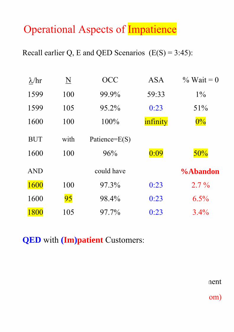
Operational Aspects of Impatience

Recall earlier Q, E and QED Scenarios (E(S) = 3:45):

/hr N OCC ASA % Wait = 0

1599 100 99.9% 59:33 1%

1599 105 95.2% 0:23 51%

1600 100 100% infinity 0%

BUT with Patience=E(S)

1600 100 96% 0:09 50%

AND could have %Abandon

1600 100 97.3% 0:23 2.7 %

1600 95 98.4% 0:23 6.5%

1800 105 97.7% 0:23 3.4%

QED with (Im)patient Customers:

The "fittest" survive and wait less – much less!

Erlang-A: Erlang-C with Exponential Patience / Abandonment

Downloadable implementation: 4CallCenters(.com)

Operational Aspects of Impatience

Recall earlier Q, E and QED Scenarios (E(S) = 3:45):

/hr N OCC ASA % Wait = 0

1599 100 99.9% 59:33 1%

1599 105 95.2% 0:23 51%

1600 100 100% infinity 0%

BUT with Patience=E(S)

1600 100 96% 0:09 50%

AND could have %Abandon

1600 100 97.3% 0:23 2.7 %

1600 95 98.4% 0:23 6.5%

1800 105 97.7% 0:23 3.4%

QED with (Im)patient Customers:

The "fittest" survive and wait less – much less!

Erlang-A: Erlang-C with Exponential Patience / Abandonment

Downloadable implementation: 4CallCenters(.com)

Operational Aspects of Impatience

Recall earlier Q, E and QED Scenarios (E(S) = 3:45):

/hr N OCC ASA % Wait = 0

1599 100 99.9% 59:33 1%

1599 105 95.2% 0:23 51%

1600 100 100% infinity 0%

BUT with Patience=E(S)

1600 100 96% 0:09 50%

AND could have %Abandon

1600 100 97.3% 0:23 2.7 %

1600 95 98.4% 0:23 6.5%

1800 105 97.7% 0:23 3.4%

QED with (Im)patient Customers:

The "fittest" survive and wait less – much less!

Erlang-A: Erlang-C with Exponential Patience / Abandonment

Downloadable implementation: 4CallCenters(.com)

Operational Aspects of Impatience

Recall earlier Q, E and QED Scenarios (E(S) = 3:45):

/hr N OCC ASA % Wait = 0

1599 100 99.9% 59:33 1%

1599 105 95.2% 0:23 51%

1600 100 100% infinity 0%

BUT with Patience=E(S)

1600 100 96% 0:09 50%

AND could have %Abandon

1600 100 97.3% 0:23 2.7 %

1600 95 98.4% 0:23 6.5%

1800 105 97.7% 0:23 3.4%

QED with (Im)patient Customers:

The "fittest" survive and wait less – much less!

Erlang-A: Erlang-C with Exponential Patience / Abandonment

Downloadable implementation: 4CallCenters(.com)

Asymptotic Operational Regimes

Example of Half-Hour ACD Report

Time Calls Answered Abandoned% ASA AHT Occ% # of agents

Total 20,577 19,860 3.5% 30 307 95.1%

8:00 332 308 7.2% 27 302 87.1% 59.3

8:30 653 615 5.8% 58 293 96.1% 104.1

9:00 866 796 8.1% 63 308 97.1% 140.4

9:30 1,152 1,138 1.2% 28 303 90.8% 211.1

10:00 1,330 1,286 3.3% 22 307 98.4% 223.1

10:30 1,364 1,338 1.9% 33 296 99.0% 222.5

11:00 1,380 1,280 7.2% 34 306 98.2% 222.0

11:30 1,272 1,247 2.0% 44 298 94.6% 218.0

12:00 1,179 1,177 0.2% 1 306 91.6% 218.3

12:30 1,174 1,160 1.2% 10 302 95.5% 203.8

13:00 1,018 999 1.9% 9 314 95.4% 182.9

13:30 1,061 961 9.4% 67 306 100.0% 163.4

14:00 1,173 1,082 7.8% 78 313 99.5% 188.9

14:30 1,212 1,179 2.7% 23 304 96.6% 206.1

15:00 1,137 1,122 1.3% 15 320 96.9% 205.8

15:30 1,169 1,137 2.7% 17 311 97.1% 202.2

16:00 1,107 1,059 4.3% 46 315 99.2% 187.1

16:30 914 892 2.4% 22 307 95.2% 160.0

17:00 615 615 0.0% 2 328 83.0% 135.0

17:30 420 420 0.0% 0 328 73.8% 103.5

18:00 49 49 0.0% 14 180 84.2% 5.8

13

Asymptotic Operational Regimes

Efficiency-Driven (ED) regime

Time Calls Answered Abandoned% ASA AHT Occ% # of agents

13:30 1,061 961 9.4% 67 306 100.0% 163.4

• 100% occupancy;

• high P{Ab};

• considerable ASA;

• P{W > 0} ≈ 1.

Offered load

RED∆=

λ

µ= 1061 :

1800

306= 180.37 .

Definition:

n = RED · (1− γ) γ > 0.

In our case, service grade

γ = 1− n

RED= 1− 163.4

180.37= 0.094 ≈ P{Ab} .

• This case is similar to traditional queues in heavy traffic;

• See recent papers of Whitt (2004).

14

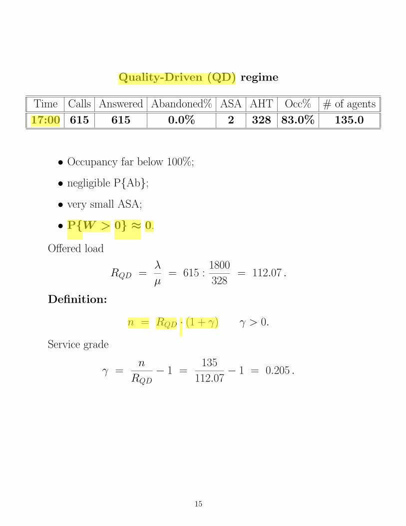
Quality-Driven (QD) regime

Time Calls Answered Abandoned% ASA AHT Occ% # of agents

17:00 615 615 0.0% 2 328 83.0% 135.0

• Occupancy far below 100%;

• negligible P{Ab};

• very small ASA;

• P{W > 0} ≈ 0.

Offered load

RQD =λ

µ= 615 :

1800

328= 112.07 .

Definition:

n = RQD · (1 + γ) γ > 0.

Service grade

γ =n

RQD− 1 =

135

112.07− 1 = 0.205 .

15

Quality and Efficiency-Driven (QED) regime

Time Calls Answered Abandoned% ASA AHT Occ% # of agents

14:30 1,212 1,179 2.7% 23 304 96.6% 206.1

• High occupancy, but not 100%;

• small P{Ab} and ASA;

• P{W > 0} ≈ α, 0 < α < 1.

RQED =λ

µ= 1212 :

1800

304= 204.69 .

Definition:

n = RQED + β√RQED , −∞ < β < ∞ .

Service grade

β =n−RQED√

RQED=

206.1− 204.69√204.69

= 0.10 .

Square-Rule Safety Staffing: Described by Erlang in 1924!

Formal analysis:

• Erlang-C: Halfin & Whitt (1981), β > 0;

• Erlang-B (M/M/n/n): Jagerman (1974);

• Erlang-A: Garnett, Mandelbaum, Reiman (2002);

• M/M/n+G: Present thesis.

16

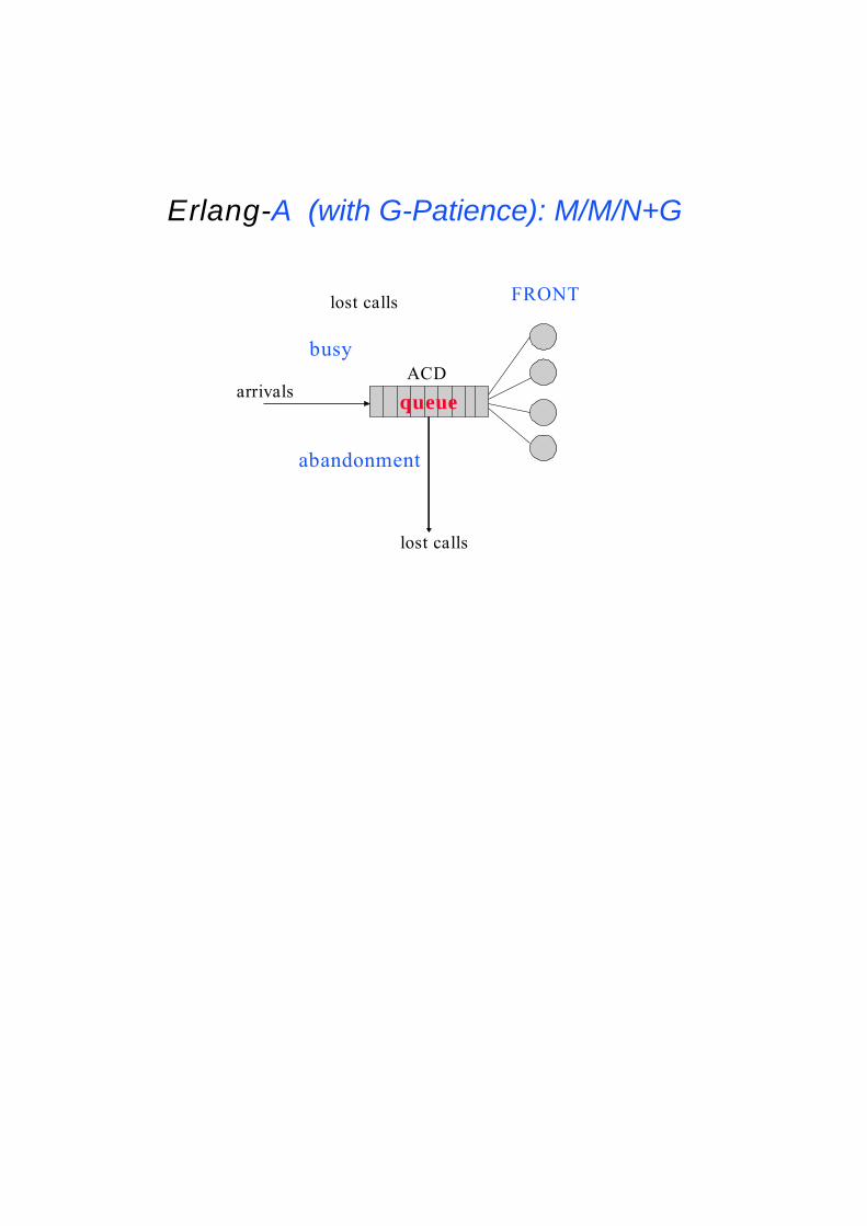
Erlang-A (with G-Patience): M/M/N+G

lost calls

arrivals

lost calls

abandonment

busy

FRONT

queue

ACD

QED Theorem (Garnett, M. and Reiman '02; Zeltyn '03)

Consider a sequence of M/M/N+G models, N=1,2,3,…

Then the following points of view are equivalent:

• QED %{Wait > 0} ≈ α , 0 < α < 1 ;

• Customers %{Abandon} ≈ Nγ , 0 < γ ;

• Agents OCC Nγβ +

−≈ 1 −∞ < β < ∞ ;

• Managers RRN β+≈ , ×= λR E(S) not small;

QED performance (ASA, ...) is easily computable, all in terms

of β (the square-root safety staffing level) – see later.

Covers also the Extremes:

α = 1 : N = R - γ R Efficiency-driven

α = 0 : N = R + γ R Quality-driven

QED Approximations (Zeltyn)

λ – arrival rate,

µ – service rate,

N – number of servers,

G – patience distribution,

g0 – patience density at origin (g0 = θ, if exp(θ)).

N = λµ + β

√λµ + o(

√λ) , −∞ < β < ∞ .

P{Ab} ≈ 1√N

· [h(β̂) − β̂] ·

[õ

g0+

h(β̂)

h(−β)

]−1

,

P

{W >

T√N

}≈

[1 +

√g0

µ· h(β̂)

h(−β)

]−1

· Φ̄(β̂ +

√g0µ · T )

Φ̄(β̂),

P

{Ab

∣∣∣∣ W >T√N

}≈ 1√

N·√

g0

µ· [h (

β̂ +√

g0µ · T ) − β̂]

.

Here

β̂ = β

õ

g0

Φ̄(x) = 1 − Φ(x) ,

h(x) = φ(x)/Φ̄(x) , hazard rate of N(0,1).

• Generalizing Garnett, M., Reiman (2002) (Palm 1943–53)

• No Process Limits

Efficiency-Driven Approximations

(Zeltyn; Whitt)

G = (Im)Patience distribution

N = λµ

· (1 − γ) + o(λ) , γ > 0.

Assume the equation

G(x) = γ

has a unique solution x∗.

Then

P{Ab} ≈ γ (insensitive to G)

P{W > T} ≈{

1 − G(T ), T < x∗

0, T > x∗ ,

P{Ab | W > T} ≈ γ − G(T ) , 0 ≤ T < x∗ .

• Derivation: Laplace Method, based on Baccelli & Hebuterne

(1981)

• Towards Dimensioning (with Borst, Reiman)

Erlang-A: Moderate (Im)patience

M/M/N + M queue, with

service rate µ equals abandonment rate

Lt: number-in-system at time t (Birth & Death)

For any N, transition-rates for {Lt, t 0}:

Note: The same transition rates as M/M/

0 1 N N+12

µ 2µ

……… N-1

Nµ

.....

Nµ+

(N+1)µ

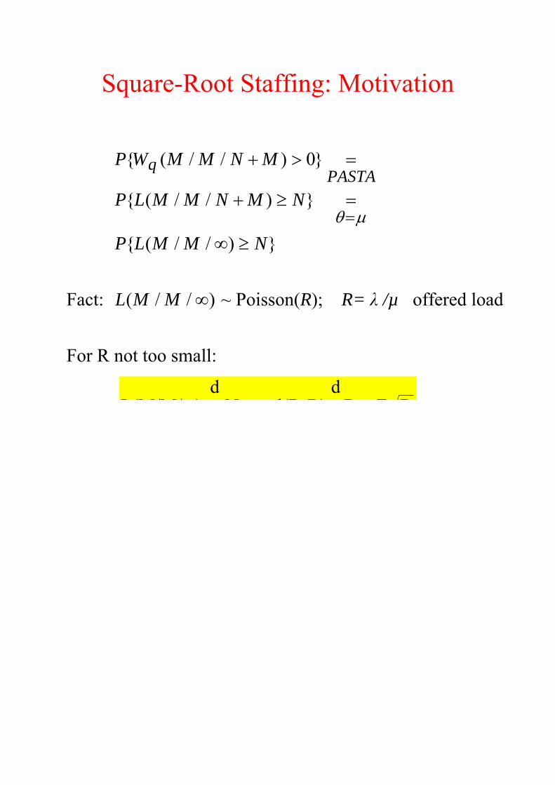
Square-Root Staffing: Motivation

})//({

})//({

}0)//({

NMMLP

NMNMMLP

MNMMWPPASTA

q

Fact: )//( MML ~ Poisson(R); R= /µ offered load

For R not too small:

RZRd

R)Normal(R,d

)L(M/M/

R

RN

R

RNq ZPWP 1}0{

Given target delay-probability = R

RN1

RRN , with )1(1

N is the "least integer for which" }0{ qWP

Square-Root Staffing: Motivation

})//({

})//({

}0)//({

NMMLP

NMNMMLP

MNMMWPPASTA

q

Fact: )//( MML ~ Poisson(R); R= /µ offered load

For R not too small:

RZRd

R)Normal(R,d

)L(M/M/

R

RN

R

RNq ZPWP 1}0{

Given target delay-probability = R

RN1

RRN , with )1(1

N is the "least integer for which" }0{ qWP

Square-Root Staffing: Motivation

})//({

})//({

}0)//({

NMMLP

NMNMMLP

MNMMWPPASTA

q

Fact: )//( MML ~ Poisson(R); R= /µ offered load

For R not too small:

RZRd

R)Normal(R,d

)L(M/M/

R

RN

R

RNq ZPWP 1}0{

Given target delay-probability = R

RN1

RRN , with )1(1

N is the "least integer for which" }0{ qWP

Erlang-A: P{Wait>0}= vs. (N=R+ R)

0

0.1

0.2

0.3

0.4

0.5

0.6

0.7

0.8

0.9

1

-3 -2.5 -2 -1.5 -1 -0.5 0 0.5 1 1.5 2 2.5 3

P{W

ait

>0

}

Halfin-Whitt GMR(0.1) GMR(0.5) GMR(1) GMR(2)

GMR(5) GMR(10) GMR(20) GMR(50) GMR(100)

GMR(x) describes the asymptotic probability of delay as a function of when

x . Here, and µ are the abandonment and service rate, respectively.

Erlang-A: P{Abandon}* N vs.

0

0.2

0.4

0.6

0.8

1

1.2

1.4

1.6

1.8

2

2.2

2.4

2.6

2.8

3

3.2

-3 -2.5 -2 -1.5 -1 -0.5 0 0.5 1 1.5 2 2.5 3

P{A

ba

nd

on

}*N

GMR(0.1) GMR(0.5) GMR(1) GMR(2) GMR(5)

GMR(10) GMR(20) GMR(50) GMR(100)

Designing a Call Center

Approximate Performance Measures

P{Wait > 0} ≈1 +

√√√√√θ

µ· h(β̂)

h(−β)

−1

E[Wait|Wait > 0] ≈ 1√N·√√√√√ 1

θµ·[h(β̂)− β̂

]

P{Ab} ≈ 1√N·√√√√√θ

µ·[h(β̂)− β̂

]·1 +

√√√√√θ

µ· h(β̂)

h(−β)

−1

P{Ab|Wait > 0} ≈ 1√N·√√√√√θ

µ·[h(β̂)− β̂

]

P

Wait

E[S]>

t√N

∣∣∣∣∣∣∣ Wait > 0

∼Φ̄(β̂ +

√θµ · t

)

Φ̄(β̂)

P

Ab

∣∣∣∣∣∣∣Wait

E[S]>

t√N

≈ 1√N·√√√√√θ

µ·h

β̂ + t

√√√√√θ

µ

− β̂

E

Wait

E[S]

∣∣∣∣∣∣∣ Ab

≈ 1√N· 1

2

√√√√µ

θ· 1

h(β̂)− β̂− β̂

Here

β̂ = β

√√√√µ

θ,

Φ̄(x) = 1− Φ(x) ,

h(x) = φ(x)/Φ̄(x) , hazard rate of N(0, 1).

1

40

54

Fitting a Simple Model to a Complex Reality

41

55

QED Dimensioning: ⋅ Safety-Staffing Dimensioning, with Borst, Reiman and Zeltyn: Asymptotically optimal - safety staffing (conjectured).

RryRN ⋅⎟⎠

⎞⎜⎝

⎛+≈

µθ;*

=r cost of delay / cost of staffing;

⎟⎠

⎞⎜⎝

⎛µθ;* ry = optimal service grade: independent of λ !

As 0↓θ , ⎟⎠

⎞⎜⎝

⎛µθ;* ry increases to )(* ry (M/M/N).

Note: µθ

<r implies that “no service” is optimal.

42

56

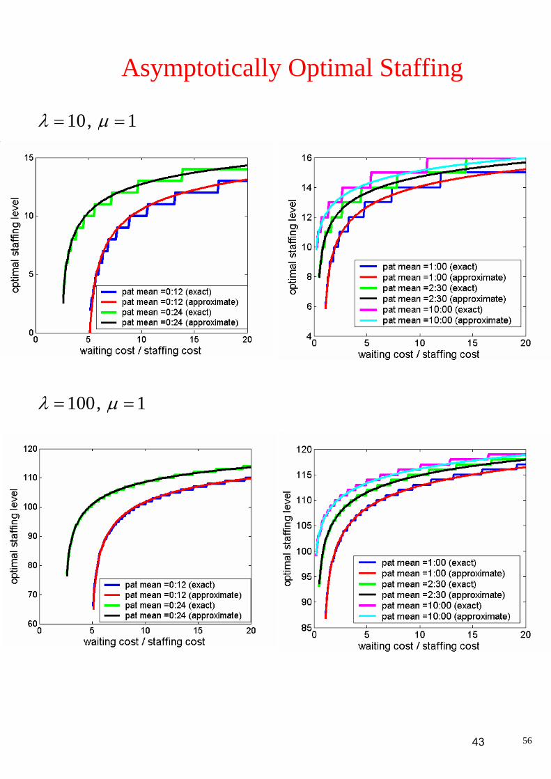
Asymptotically Optimal Staffing

10=λ , 1=µ

100=λ , 1=µ

43

57

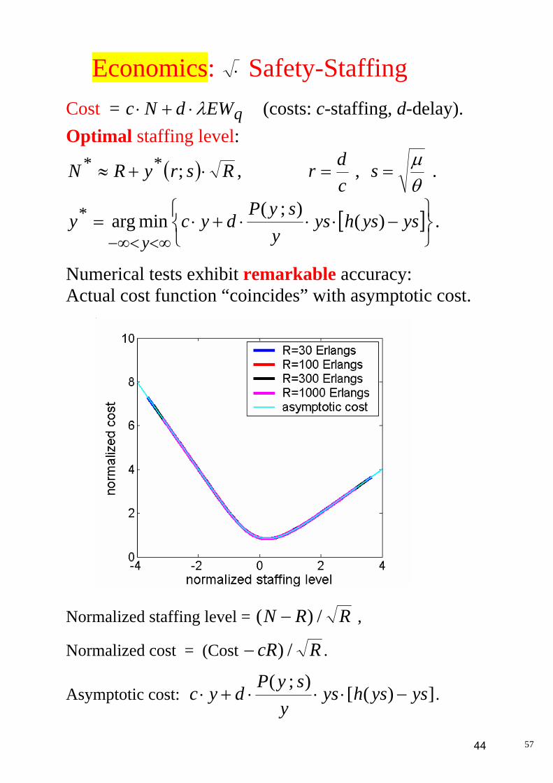
Economics: ⋅ Safety-Staffing Cost = qEWdNc λ⋅+⋅ (costs: c-staffing, d-delay). Optimal staffing level:

( ) RsryRN ⋅+≈ ;** , cdr = ,

θµ

=s .

[ ]⎭⎬⎫

⎩⎨⎧

−⋅⋅⋅+⋅=∞<<∞−

ysyshysy

syPdycy

y)(

);(minarg* .

Numerical tests exhibit remarkable accuracy: Actual cost function “coincides” with asymptotic cost.

Normalized staffing level = RRN /)( − ,

Normalized cost = (Cost RcR /)− .

Asymptotic cost: ])([);(

ysyshysy

syPdyc −⋅⋅⋅+⋅ .

44