Empirical Regression Quantile Process in Analysis of Riskweb/@inf/@math/... · exposures to toxic...

Introduction RQ Ave RQ Two-step RQ Applications References

Empirical Regression Quantile Process inAnalysis of Risk

Jana Jurecková

Charles University, Prague

ICORS, Wollongong 2017

Jurecková, Schindler, Picek Empirical Regression Quantile Process in Analysis of Risk


Joint work with Martin Schindler and Jan Picek,

Technical University Liberec



1 Introduction

2 RQAveraged regression quantile

3 Ave RQAveraged regression quantile process

4 Two-step RQ

5 Applications

6 References



Outline

We consider the problem of the loss Yi under realization xi ,representing economic and market variables. The xi caninvolve exogenous economic and market variables, the pastobserved returns, etc. Such investigation we meet in thefinance, in the insurance and in the social statistics. However,the risks also appear in the environment analysis, dealing withexposures to toxic chemicals (coming from power plants, roadvehicles, from agriculture), and in other situations. For the latterproblems we refer for a nice review to Molak (1997).More definitions of coherent risk measures, even satisfying asuitable axiomatic structure, appeared in the literature. Fordiscussions and some projects we refer to Acerbi and Tasche(2002), Artzner(1997,1999), Cai and Wang (2008), Chan(2015), Pflug (2000), Rockafellar, Royset, Miranda (2014),Rockafellar and Uryasev (2001, 2013), Tasche (2000), Trindadeet al. (2007), Uryasev (2000), and to other papers cited in.



The expected shortfall, based on quantiles of a portfolio returnor of an asset, is a generally accepted measure of the financialor other risk. Acerbi and Tasche (2002) call it the "expectedloss in the 100α% worst cases", or shortly the "expectedα-shortfall", 0 < α < 1. It is defined as

− IE{Y |Y ≤ F−1(α)} = −1α

∫ α

0F−1(u)du, (1)

where F is the distribution function of the asset Y . Thischaracteristic can be estimated through approximations of thequantile function F−1(u) based on the sample quantiles.Our challenge to quantify the risks with the aid of probabilisticrisk assessment. A a convenient tool for the global riskmeasurement in such situations is provided by the averagedregression quantile, introduced by Jurec. and Picek (2014), orby its two-step modification.



As a model for the relation of the loss to covariates we considerthe regression model

Yni = β0 + x⊤niβ + eni , i = 1, . . . , n (2)

where Yn1, . . . , Ynn are observed responses, en1, . . . , enn areindependent model errors, possibly non-identically distributedwith unknown distribution functions Fi , i = 1, . . . , n. Thecovariates xni = (xi1, . . . , xip)⊤, i = 1, . . . , n are random ornonrandom, and β∗ = (β0, β

⊤)⊤ = (β0, β1, . . . , βp)⊤ ∈ Rp+1 is

an unknown parameter. For the sake of brevity, we also use thenotation x∗

ni = (1, xi1, . . . , xip)⊤, i = 1, . . . , n.

An important tool in the risk analysis isthe regression α-quantile

β∗

n(α) =(βn0(α), (βn(α))⊤

)⊤

=(βn0(α), βn1(α), . . . , βnp(α)

)⊤

.


Introduction RQ Ave RQ Two-step RQ Applications ReferencesAveraged regression quantile

Regression quantile

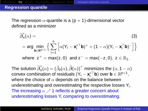
The regression α-quantile is a (p + 1)-dimensional vectordefined as a minimizer

β∗

n(α) = (3)

= arg minb∈IRp+1

{ n∑

i=1

[α(Yi − x∗⊤

i b)+ + (1 − α)(Yi − x⊤i b)−

]}

where z+ = max(z, 0) and z− = max(−z, 0), z ∈ R1.

The solution β∗

n(α) = (β0(α), β(α))⊤ minimizes the (α, 1 − α)convex combination of residuals (Yi − x∗⊤

i b) over b ∈ Rp+1,

where the choice of α depends on the balance betweenunderestimating and overestimating the respective losses Yi .

The increasing α ր 1 reflects a greater concern aboutunderestimating losses Y, comparing to overestimating.



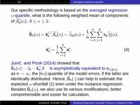
Our specific methodology is based on the averaged regressionα-quantile, what is the following weighted mean of componentsof β

∗

n(α), 0 ≤ α ≤ 1:

Bn(α) = x∗⊤n β

∗

n(α) = βn0(α) +1n

n∑

i=1

p∑

j=1

xij βj(α),

x∗n =

1n

n∑

i=1

x∗i . (4)

Jurec. and Picek (2014) showed thatBn(α) − β0 − x⊤

n β is asymptotically equivalent to en:[nα]

as n → ∞, the [nα]-quantile of the model errors, if the latter areidentically distributed. Hence, Bn(·) can help to estimate theexpected α-shortfall (1) even under the nuisance regression.Besides Bn(α), we also use its various modifications, bettercomprehensible and easier for calculation.



Our methods are nonparametric, thus applicable also toheavy-tailed and skewed distribution. Braione and Scholtes(2016) tried to forecast the value-at-risk under differentdistributional assumptions and speak about considerableimprovement over normality.An extension to autoregressive models is possible and worththe further study; the main tool will be the autoregressionquantiles, introduced by Koul and Saleh (1995), and theiraveraged versions. The autoregression quantile will reflect thevalue-at-risk, based on the past assets, while its averagedversion will try to mask the past history.The behavior of Bn(α) with 0 < α < 1 has been illustrated byBassett (1988) and Koenker and Bassett (1982), andsummarized by Koenker (2005); it is showed that Bn(α) isnondecreasing step function of α ∈ (0, 1).



The extreme averaged regression quantile Bn(1) with α = 1was studied by Jurecková (2016); this reflects greater concernabout underestimating losses Y , rather than overestimating.The upper bound of the number Jn of breakpoints of β

∗

n(·) and

also of Bn(·) is(

np + 1

)= O

(np+1

). However, Jn may be

much smaller; Portnoy (1991) showed that, under someconditions on the design matrix Xn, the number of breakpointsJn is of order Op(n log n), as n → ∞.

An alternative to the regression quantile is the two-stepregression α-quantile, introduced by Jurec. and Picek (2005).Here the slope components β are estimated by a specificrank-estimate βnR, which is invariant to the shift in location.The intercept component is estimated by the α-quantile ofresiduals Yi − x⊤

i βnR, i = 1, . . . , n.



The averaged two-step regression quantile Bn(α) isasymptotically equivalent to Bn(α), as n → ∞, under a widechoice of the R-estimators of the slopes. Its finite-samplebehavior of Bn(α) is affected, but generally rather slightly, bythe choice of R-estimator.

The averaged two-step regression quantile Bn(α) is astep-function of α ∈ (0, 1), and can be made monotone in α bya suitable choice of R-estimate βnR. Hence, then we canconsider its inversion, which in turn estimates the parentdistribution F of the model errors. It is simpler than theinversion of Bn(α), and as such it is convenient for an inference.



Empirical quantile estimates based on Bn and on Bn andapproximations of parent distribution function F by theirinversions are numerically illustrated in Jurec., Schindler andPicek (2017).The empirical quantile approximations of the normal, Cauchyand generalized extreme value (GEV) distribution functionsappear to be very good. In the case of two-step regressionquantile Bn(α), it is preferred to use an R-estimator of β,

generated by a score function, skew-symmetric on (0, 1) whichworks even under F skewed or heavy-tailed.


Introduction RQ Ave RQ Two-step RQ Applications ReferencesAveraged regression quantile process

Behavior of Bn(α)

Consider again the minimization (3), α ∈ [0, 1] fixed, leading tothe regression quantile β(α). This was treated by Koenker andBassett (1978) as a special linear programming problem.Various modifications of this algorithm were developed by moreauthors. Its dual program is a parametric linear program, whichcan be written simply as

maximize Y⊤n a(α)

under X∗⊤n a(α) = (1 − α)X∗⊤

n 1⊤n (5)

a(α) ∈ [0, 1]n, 0 ≤ α ≤ 1

where

X∗n =

x∗⊤n1

. . .

x∗⊤nn

is of order n × (p + 1). (6)



The components of the optimal solutiona(α) = (an1(α), . . . , ann(α))⊤ of (5), called regression rankscores, were studied by Gutenbrunner and Jurec. (1992), whoshowed that ani(α) is a continuous, piecewise linear function ofα ∈ [0, 1] and ani(0) = 1, ani(1) = 0, i = 1, . . . , n.

Moreover, a(α) is invariant in the sense that it does not changeif Y is replaced with Y + X∗

nb∗, ∀b∗ ∈ Rp+1. Let {x∗

i1, . . . , x∗

ip+1}

be the optimal base in (5) and let {Yi1 , . . . , Yip+1} be thecorresponding responses. Then Bn(α) equals to a weightedmean of {Yi1 , . . . , Yip+1}, with the weights based on theregressors.



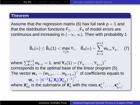
Theorem

Assume that the regression matrix (6) has full rank p + 1 andthat the distribution functions F1, . . . , Fn of model errors arecontinuous and increasing in (−∞,∞). Then with probability 1

Bn(α) ≤ Bn(1) < maxi≤n

Yi , Bn(α) =

p+1∑

k=1

wk ,αYik , (7)

where∑p+1

k=1 wk ,α = 1, and Yn(1) = (Yi1 , . . . , Yip+1)⊤

corresponds to the optimal base of the linear program (5).The vector wα = (w1,α, . . . , wp+1,α)⊤ of coefficients equals to

wα =[n−11⊤

n X∗n(X

∗n1)

−1]⊤

,

where X∗n1 is the submatrix of X∗

n with the rows x∗⊤i1

, . . . , x∗⊤ip+1

.



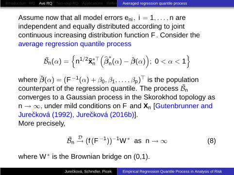
Assume now that all model errors eni , i = 1, . . . , n areindependent and equally distributed according to jointcontinuous increasing distribution function F . Consider theaverage regression quantile process

Bn(α) ={

n1/2x∗⊤n

(β∗

n(α) − β(α)); 0 < α < 1

}

where β(α) = (F−1(α) + β0, β1, . . . , βp)⊤ is the populationcounterpart of the regression quantile. The process Bn

converges to a Gaussian process in the Skorokhod topology asn → ∞, under mild conditions on F and Xn [Gutenbrunner andJurecková (1992), Jurecková (2016b)].More precisely,

BnD→ (f (F−1))−1W ∗ as n → ∞ (8)

where W ∗ is the Brownian bridge on (0,1).



The trajectories of Bn are step functions, nondecreasing inα ∈ (0, 1), and they have finite numbers of discontinuities foreach n. Bassett and Koenker (1982) showed that ifBn(α1) = Bn(α2) for 0 < α1 < α2 < 1, then α2 − α1 ≤ p+1

n withprobability 1, hence the length of interval on which is Bn(α)constant tends to 0 for n → ∞ and fixed p. Let0 < α1 < . . . < αJn < 1 be the breakpoints of Bn(α), 0 < α < 1,

and −∞ < Z1 < . . . < ZJn < ∞ be the corresponding values ofBn(αk ), k = 1, . . . , Jn. Then we can consider the inversionFn(z) of Bn(α), namely

Fn(z) = inf{α : Bn(α) ≥ z}, −∞ < z < ∞.

It is a bounded nondecreasing step function and, givenY1, . . . , Yn satisfying (2), Fn is a distribution function of arandom variable attaining values Z1, . . . , ZJn with probabilitiesequal to the spacings of α1, . . . , αJn .



Two-step regression quantile

As an alternative, we can consider the empirical process Bn(α)

based on two-step regression quantile β∗

n(α), asymptoticallyequivalent to original regression quantile β

∗

n(α) as n → ∞.

The two-step regression α-quantile β∗

n(α) treats the slopecomponents β and the intercept β0 separately. The slopecomponent part is an R-estimate βnR of β. Its advantage is thatit is invariant to the shift in location, hence independent ofintercept β0. The intercept component βn0(α) is the [nα]-orderstatistic of the residuals Yi − x⊤

i βnR, i = 1, . . . , n. The two-stepα-regression quantile is then the vector

β∗

n(α) =

(βn0(α)

βnR

)∈ R

p+1. (9)



R-estimate of slopes

The R-estimate of the slope components is generated by anondecreasing score function ϕ(u), square-integrable on (0,1).We can consider two types of rank scores, generated by ϕ :

Exact scores:

An(i) = IE{ϕ(Un:i)}, i = 1, . . . , n

where Un:1 ≤ . . . ≤ Un:n is the ordered random sample of size nfrom the uniform (0,1) distribution.

Approximate scores:

either (i) An(i) = n∫ (i+1)/n

i/n ϕ(u)du,

or (ii) An(i) = ϕ(

in+1

), i = 1, . . . , n.



The test criteria and estimates based on either of these scoresare mutually asymptotically equivalent as n → ∞. Under nfinite, the rank tests based on the exact scores are locally mostpowerful against particular alternatives.The R-estimator βnR of the slopes is a minimizer of the Jaeckel(1972) measure of rank dispersion Dn(b) :

βnR = argminb∈RpDn(b),

where Dn(b) =n∑

i=1

(Yi − x⊤i b) An(Rni(Yi − x⊤

i b)), b ∈ Rp

where Rni(Yi − x⊤i b) is the rank of the i-th residual, i = 1, . . . , n.

The typical choice are the approximate scores generated by ϕλ

with a fixed λ ∈ (0, 1):

ϕλ(u) = λ − I[u < λ], 0 < u < 1.



Define the averaged two-step regression α-quantile Bn(α) as

Bn(α) = x∗⊤n β

∗

n(α) =(

Yi − (xi − xn)⊤βnR

)

n:[nα]

hence as the [nα]-th order statistic of the residualsYi − (xi − xn)

⊤βnR , i = 1, . . . , n.

Bn(α) is scale equivariant and regression equivariant. It is astep function, nondecreasing in α ∈ (0, 1), thus invertible. It is atool for an inference on the risk under a nuisance regressionwith respect to some external factors.Bn(α) is asymptotically equivalent to Bn(α) under generalconditions, hence for each α asymptotically equivalent toen:[nα] + β0 + x⊤

n β. This is true under F with finite Fisherinformation and under standard condition on Xn, n = 1, 2, . . . .



If βnR is an√

n-consistent R-estimator of β, generated by a րsquare-integrable score function ϕ, then

(i) n1/2[(Bn(α) − β0 − xnβ) − en:[nα]

]= op(1)

(ii) n1/2∣∣∣Bn(α) − Bn(α)

∣∣∣ = op(1)

as n → ∞, uniformly over α ∈ (ε, 1 − ε) ⊂ (0, 1), ∀ε ∈ (0, 12).

The upper bound on the number Jn of breakpoints of Bn(·) isO

(np+1

), and by Portnoy (1991) it can be of order Op(n log n)

as n → ∞ under some conditions. On the other hand, Bn(α) isa ր step-function with exactly n breakpoints. Both Bn(·) andBn(·) approximate the quantile function of the model errors, andtheir inversions approximate the distribution function F , evenasymmetric. The numerical study confirms these facts evenunder small sample sizes. As such, both processes can beused in estimation of various measures of risk, forgoodness-of-fit testing, as well in the estimation of the tails.



Applications: Exposure to chemical agents

The applications are not only for the financial risk, but also inthe analysis of the human health risk from the exposures totoxic chemicals (coming from power plants, road vehicles, fromthe agriculture, and others).L. Wallace (1996) describes a study of level of the benzeneexposures due to its major sources, as active and passivesmoking, auto exhaust, and driving or riding in automobiles.The study follows dependence on the climate season, on dayand night, on geographic regions, smoker/nonsmoker and otherfactors.



Bennett et al. (2011) is a detailed a study of aspects ofventilation and levels of indoor air pollutants in California.exchange rate It compares the air in various types of building,as healthcare establishments, gyms, offices, hair salons, retailstores, restaurants and gas stations. It involves also themeasurement of the black carbon ratio, aldehydes and volatileorganic compounds.Kopelovich et al. (2015) studied the human health risk due toexposition of toluene and dibutyl phthalate in some workenvironments.



References

Acerbi, C. and Tasche, D. (2002). Expected shortfall: A naturalcoherent alternative to value at risk, Economic Notes 31,379-388

Artzner, P., Delbaen, F., Eber, J.-M., Heath, D. (1997). Thinkingcoherently. RISK 10 (11)

Artzner, P., Delbaen, F., Eber, J.-M., Heath, D. (1999). Coherentmeasures of risk. Math. Fin. 9, 203–228

Bassett, G.W. Jr. (1988). A property of the observations fit bythe extreme regression quantiles. Comp. Stat. Data Anal. 6,353–359

Bassett, G. W. and Koenker, R. W. (1982). An empiricalquantile function for linear models with iid errors. J. Amer.Statist. Assoc. 77, 405–415.



Bennett, D., Wu, X., Trout, A., Apte, M., Faulkner, D.,Maddalena, R., Sullivan., D. (2011). Indoor environmentalquality and heating, ventilating, and air conditioning survey ofsmall and medium size commercial buildings. Fields Study.Public Interest Energy Research (PIER) Program. FinalCollaborative Report

Cai, Z. and Wang, X., (2008). Nonparametric estimation ofconditional VaR and expected shortfall, Journal ofEconometrics 147, 120–130

Chan, J. S .K., (2015). Predicting loss reserves using quantileregression [Quantile regression loss reserve models], Journalof Data Science 13, 127–156

Gutenbrunner, C. and J. Jurecková (1992). Regression rankscores and regression quantiles. Ann.Statist. 20 : 305–330.



Jaeckel, L. A. (1972). Estimating regression coefficients byminimizing the dispersion of the residuals. Ann. Math. Statist.43, 1449–1459.

Jurecková, J. (2016). Finite sample behavior of averagedextreme regression quantile. EXTREMES 19, 41-49.

Jurecková, J. and Picek, J. (2005). Two-step regressionquantiles. Sankhya 67, Part 2, 227–252.

Jurecková, J. and Picek, J. (2012). Regression quantiles andtheir two-step modifications. Statistics and Probability Letters82, 1111–1115.

Jurecková, J. and Picek, J. (2014). Averaged regressionquantiles. In: Contemporary Developments in Statistical Theory(S. N. Lahiri et al. (eds.), Springer Proceedings in Mathematics& Statistics 68, Ch. 12, pp.203–216.



Kopelovich, L., Perez, A.L., Jacobs,N., Mendelsohn, E. (2015).Screening-level human health risk assessment of toluene anddibutyl phthalate in nail lacquers. Food and ChemicalToxicology 81, 46–53

Koenker, R. (2005). Quantile Regression. CambridgeUniversity Press.

Koenker, R. and G. Bassett (1978). Regression quantiles.Econometrica 46 : 33–50.

Koul, H. L. and Saleh, A. K. Md. E., (1995). Autoregressionquantiles and related rank-scores processes. Ann. Statist. 23,670–689

Molak, V. (ed.) (1997) Fundamentals of risk analysis and riskmanagement, CRC Press.



Pflug, G. (2000). Some remarks on the value-at-risk and theconditional value-at-risk. In, Uryasev, S. (Editor) ProbabilisticConstrained Optimization: Methodology and Applications.Kluwer Academic Publishers

Portnoy, S. (1991). Asymptotic behavior of the number ofregression quantile breakpoints. SIAM Journal on Scientific andStatistical Computing 12/4, 867–883.

Rockafellar, R.T., Uryasev, S. (2001). Conditional Value-at-Riskfor general loss distributions. Research report 2001-5, ISEDepart., University of Florida

Rockafellar, R. T. and Uryasev, S., (2013). The FundamentalRisk Quadrangle in Risk Management, Optimization andStatistical Estimation, Surveys in Operations Research andManagement Science 18, 33–53



Rockafellar, R. T., Royset, J. O., Miranda, S. I. (2014).Superquantile regression with applications to buffered reliability,uncertainty quantification, and conditional value-at-risk,European Journal of Operational Research 234, 140–154

Tasche, D. (2000). Conditional expectation as quantilederivative. Working paper, TU München

Trindade, A. A., Uryasev, S. Shapiro, A. Zrazhevsky, G., (2007).Financial prediction with constrained tail risk, Journal ofBanking & Finance 31, 3524-3538

Uryasev, S. (2000). Conditional Value-at-Risk: OptimizationAlgorithms and Applications. Financial Engineering News 2/3

Wallace, L. (1996). Environmental Exposure to Benzene: AnUpdate. Environmental Health Perspectives 104, Supplement6, 1129–1136.


Empirical Regression Quantile Process in Analysis of Riskweb/@inf/@math/... · exposures to toxic...

Documents

Transcript of Empirical Regression Quantile Process in Analysis of Riskweb/@inf/@math/... · exposures to toxic...