Empirical Methods for Corporate Finance -...
58
Panel Data, Fixed Effects, and Standard Errors Empirical Methods for Corporate Finance
Transcript of Empirical Methods for Corporate Finance -...

Panel Data, Fixed Effects, and Standard Errors
Empirical Methods for Corporate Finance

The use of panel datasets
4/20/2015 2
Source: Bowen, Fresard, and Taillard (2014)

The use of panel datasets
4/20/2015 3
Source: Bowen, Fresard, and Taillard (2014)
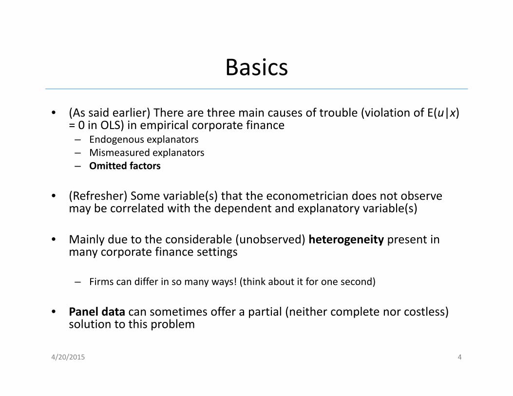
Basics
• (As said earlier) There are three main causes of trouble (violation of E(u|x) = 0 in OLS) in empirical corporate finance– Endogenous explanators– Mismeasured explanators– Omitted factors
• (Refresher) Some variable(s) that the econometrician does not observe may be correlated with the dependent and explanatory variable(s)
• Mainly due to the considerable (unobserved) heterogeneity present in many corporate finance settings
– Firms can differ in so many ways! (think about it for one second)
• Panel data can sometimes offer a partial (neither complete nor costless) solution to this problem
4/20/2015 4
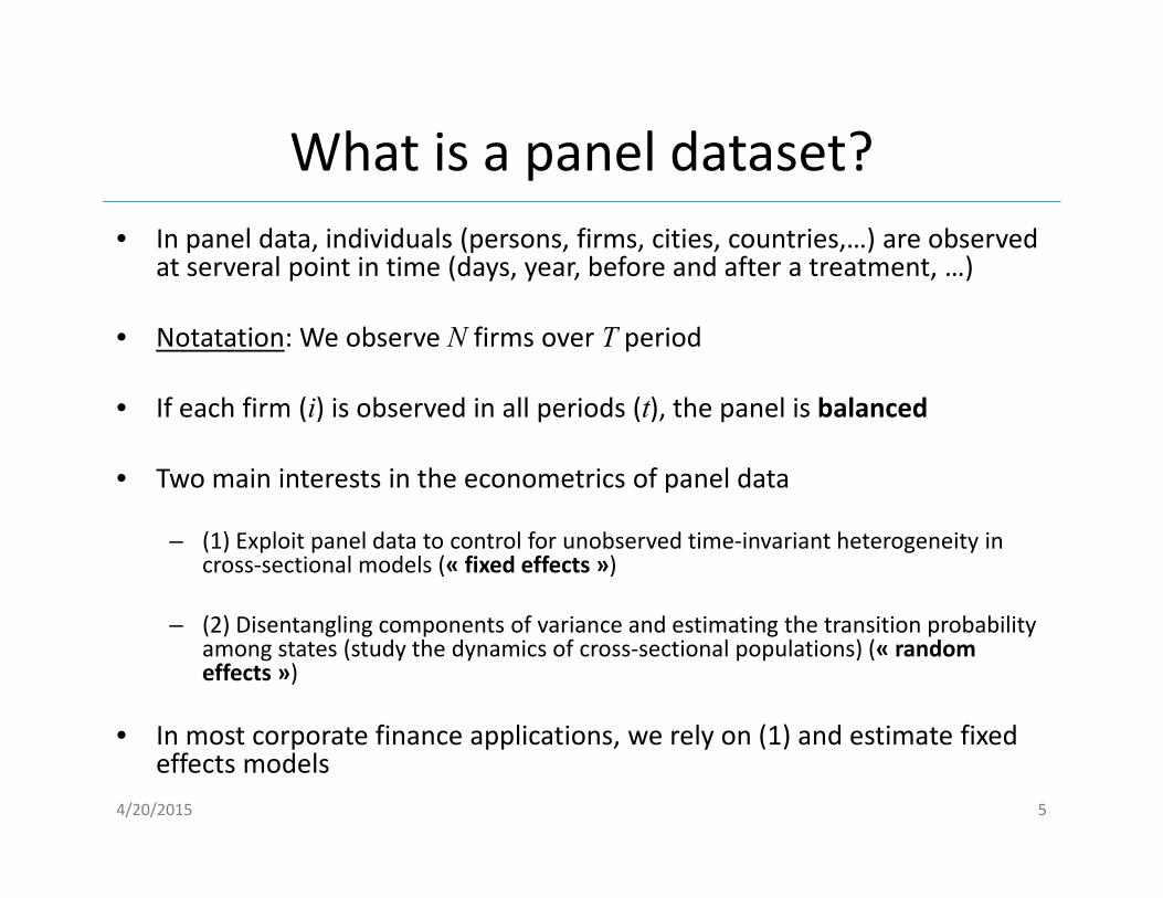
What is a panel dataset?• In panel data, individuals (persons, firms, cities, countries,…) are observed
at serveral point in time (days, year, before and after a treatment, …)
• Notatation: We observe N firms over T period
• If each firm (i) is observed in all periods (t), the panel is balanced
• Two main interests in the econometrics of panel data
– (1) Exploit panel data to control for unobserved time‐invariant heterogeneity in cross‐sectional models (« fixed effects »)
– (2) Disentangling components of variance and estimating the transition probabilityamong states (study the dynamics of cross‐sectional populations) (« randomeffects »)
• In most corporate finance applications, we rely on (1) and estimate fixedeffects models
4/20/2015 5

General structure of a panel
• The T observations for firm i can be written as
• And NT observations for all firms and time periods as
4/20/2015 6

Econometric specification: the logic
• Suppose a cross‐sectional model of the form (« the truth »)
• If ci is observed then β can be identified from a multiple regression of y on x and c
• If ci is not observed, causal identification of β requires
– Lack of correlation between xi1 and ci(« random effect »)
– An instrument (zi) uncorrelated with ui1 and ci
4/20/2015 7
0),|( with 11111 iiiiiii cxuEucxy
)(),(
1
11
i
ii
xVaryxCov
),(),(
1
11
ii
ii
xzCovyzCov

Econometric specification: the logic
• Suppose that neither of these two options is available but weobserve yi2 and xi2 for the same firm in a second period (T=2)
• Then β is identified in the regression in first difference even if ci is not observed
• And
4/20/2015 8
0),,|( 2,1222 iiiitiiii cxxuEucxy with
)()( 12,1212 iiiiii uuxxyy
)(),(
2
22
i
ii
xVaryxCov
Taking the first difference eliminate the time‐invariant unobservedheterogeneity!
The variation that identifies βis within‐firm variation

Illustration
4/20/2015 9
This is the line we wouldfit if we do not accountfor individual effects(Pooled OLS on a large cross‐section)
This is the « true » unbiased slope (thataccount for the individualeffects)
Estimation with pooled OLS is biased and inconsistent!

Why might fixed effects arise?
• Any time‐invariant individual characteristic that cannot be observed in the data at hand could contribute to the presence of fixed effects
• In regressions aimed at understanding firm behavior, specific sources of fixed effects depend on the application
• In capital structure regression (e.g. leverage) a fixed effect might be related to
– Unobserved technological differences across firms
– Unobserved ability of the CEO or people deciding on financial policies
• In general, a fixed effect can capture any low frequency unobserved variable
4/20/2015 10
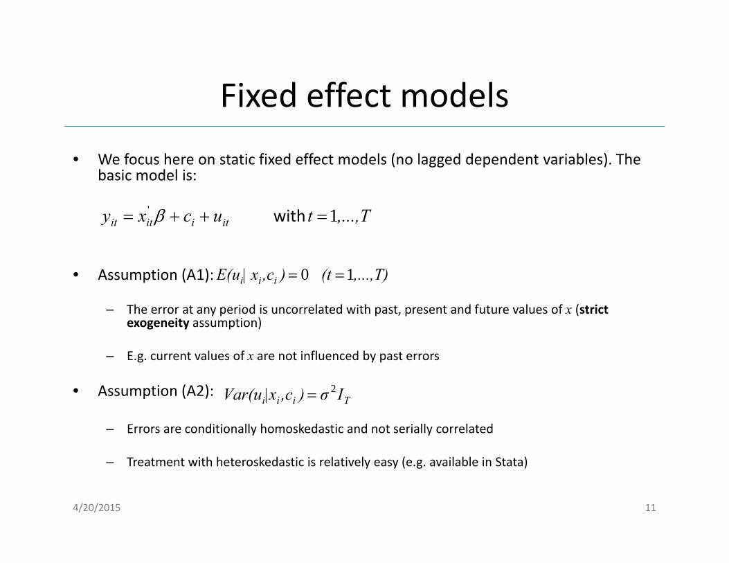
Fixed effect models• We focus here on static fixed effect models (no lagged dependent variables). The
basic model is:
• Assumption (A1):
– The error at any period is uncorrelated with past, present and future values of x (strict exogeneity assumption)
– E.g. current values of x are not influenced by past errors
• Assumption (A2):
– Errors are conditionally homoskedastic and not serially correlated
– Treatment with heteroskedastic is relatively easy (e.g. available in Stata)
4/20/2015 11
,...,Ttucxy itiitit 1' with
,...,T)(t),c| xE(u iii 10
Iσ),c|xVar(u Tiii2

Estimation with fixed effects (1)• Under A1 (mean independence), we can estimate the model in first difference by
OLS (convenient)
– OLS estimator will be unbiased and consistent (for large N)
– This is rarely the case (Cov(∆uit ,∆uit-1) is not zero!)
• If Cov(∆uit ,∆uit-1) is not zero, the optimal estimator is given by generalized least‐squares (GLS)
– Take deviation from the mean!
– Estimate the following (within or FE) specification
– Note that the firm‐specific effect (ci) dissapears (constant)
– Time‐invariant hetegeneity is solved
4/20/2015 12
yyyT
yyuxy itT
t itititititit 1' 1~~~~ with The variation that identifies β is
within‐firm variation

Estimation with fixed effects (2)• The FE estimator is asymptotically normally distributed so that the usual OLS
inference can be applied
– The usual tests (t, Wald,…) can be used in large and small samples
– In practice, the error is often likely serially correlated (T >2). This needs to be corrected (usingcluster‐robust standard errors)
• Note that time‐invariant regressors (e.g. the constant) cancel so their effect cannotbe estimated with a within estimator
• The FE estimator is numerically identical to pool OLS including a set of N-1 dummyvariables which identifies the firms and hence N-1 parameters (« Least Squares Dummy Variables Estimator » LSDV)
– Get estimates for ci
– The LSDV estimator is generally not consistent as the number of parameter goes to infinity
– F‐test for the joint significance of fixed effects (this is useful)
4/20/2015 13

Alternative: random effects
• In the FE specification, the firm‐specific effect (ci) is allowed to becorrelated with the explanatory variables (Note that this is the root of the problem!)
• If the firm‐specific effect (ci) is uncorrelated with the explanatory variables (past, present and future), we have a random effect (RE) specification
• In RE specification, the emphasis is on the error term
– The error term has two components (ci + ui) that are unrelated to the regressors
– No problem to identify β (identified in the cross‐section) but the panel structrue isused to identify the variance of ci and ui
– Used to separate out permanent from transitory components of variation
– Not many application of RE models in corporate finance
4/20/2015 14

Fixed or random effects?
• Intuitively, we should opt for a RE specification if one can be sure that the firm‐specific effect really is unrelated to the explanatory variables
• This can be tested using a (Durbin‐Wu‐) Hausmann test
• Comparision of the FE and RE estimators:
• Where J is the number of time‐varying regressors
• The null hypothesis is that the firm‐specific effect (ci) is uncorrelated withthe regressors and the errors are equicorrelated
4/20/2015 15
2~)ˆˆ)](ˆ(ˆ)ˆ(ˆ[)'ˆˆ( JOLSIVOLSIVOLSIV VVH

Implementation in Stata (1)
4/20/2015 16

Implementation in Stata (2)
4/20/2015 17

Implementation in Stata (3)
4/20/2015 18

Practical issues (1)
• Most of the empirical corporate finance use fixed effects. Is that fine?
• The answer is not obvious. The use of FE deserves careful thoughts…
• Always try estimations with fixed and random effects and check for statistical significance of the FE
• Check if the inclusion of fixed effects changes the magnitude of the coefficients in an economically meaningful way
– The inclusion of fixed effects reduces efficiency
– Even if the Hausman test rejects the null of random effects, if the economic significance is little changed, using OLS can still be valid
– E.g. Lemmon, Roberts and Zender (JoF 2008)
4/20/2015 19
Practical issues (2)
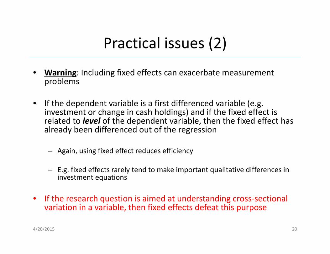
• Warning: Including fixed effects can exacerbate measurement problems
• If the dependent variable is a first differenced variable (e.g. investment or change in cash holdings) and if the fixed effect is related to level of the dependent variable, then the fixed effect has already been differenced out of the regression
– Again, using fixed effect reduces efficiency
– E.g. fixed effects rarely tend to make important qualitative differences in investment equations
• If the research question is aimed at understanding cross‐sectional variation in a variable, then fixed effects defeat this purpose
4/20/2015 20
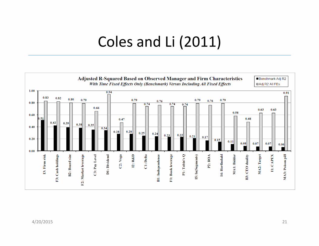
Coles and Li (2011)
4/20/2015 21

4/20/2015 22

4/20/2015 23

4/20/2015 24

4/20/2015 25
4/20/2015 26

4/20/2015 27
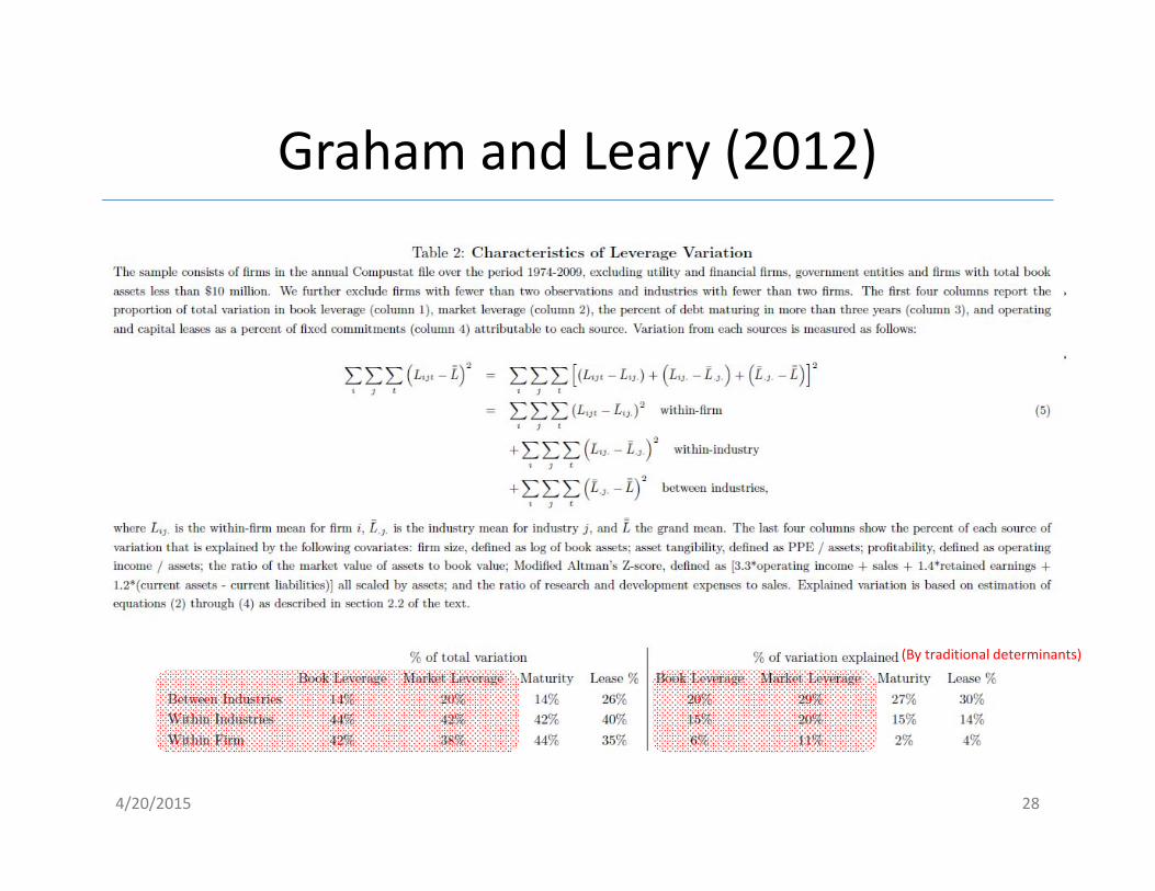
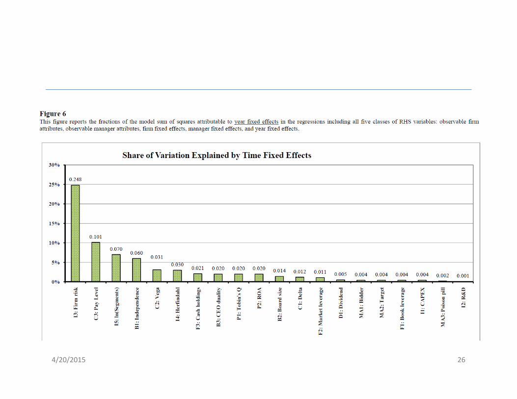
Graham and Leary (2012)
4/20/2015 28
(By traditional determinants)

Graham and Leary (2012)
4/20/2015 29

Graham and Leary (2012)
4/20/2015 30

Application: Managing with style
• Bertrand and Schoar, 2003, Managing with style: The effect of managers on firmpolicies (Quarterly Journal of Economics)
• Question: How much do individual managers matter for firm behavior and economicperformance?
• Motivation: Previous studies focused on firm‐, industry‐, and market‐levelcharacteristics to explain corporate behaviors
– View in the business press is that (certain) managers are key factors in corporate practices (e.g. Steve Jobs)
– Can add to our understanding of corporate finance
• Empirical challenge: Identify/measure the (marginal & causal) impact of managers on firms
• Empirical strategy: Use managers fixed effects to uncover their impact on variouspolicies (no causal statement here)
• Results: Managers traits appear to be related to firms choices and performance
4/20/2015 31

Location in the field
4/20/2015 32
Governance Real decisions
Financing Valuation
Institutional framework: laws, regulations, taxes, markets, macro‐economy
No causal effects here

Why should manager matter? (in theory)
• No effect (Null hypothesis)
– In a purely neoclassical view of the firm, managers are homogenous and selfless inputs intothe production process (remember your microeconomic classes…)
– Managers can differ (preferences, risk‐aversion, skills, …) but do not affect corporate policies
• Non‐zero effect (managers matter)
– Agency models (principal‐agent) allow for managers having discretion inside the firm (dependon governance practices only)
– Some models allow managers to differ
• Agency perspective (1): Managers may matter if the corporate control is poor or limited
• (improved) Neoclassical perspective (2): Firms (e.g. boards) select specific managers (endogenousmatching)
• Both approaches predict that managers matter!
4/20/2015 33

Sample construction
• Construction of a manager‐firmmatched panel dataset that tracksdifferent managers across different firms and time (why is this key?)
• Data sources
– Forbes 800 files (1969‐1999) and Execucomp (1992‐1999) for the information about CEO (and other top executives)
– Focus on CEO but also CFO, COO and subdivision CEOs
– Restrict on the subset of firms for which at least one executive can beobserved in at least one other firm (for minimum three years)
– The resulting sample contains about 600 firms and 500 managers
4/20/2015 34

Summary statistics (representative?)
4/20/2015 35
Firms in the sample are somewhat special (e.g. larger) due to data screening
The effects documentedin the paper may not generalize to smaller(private) firms
Executives from largerfirms are more likely to move betweenCOMPUSTAT firms (be in the sample)

Job transition
4/20/2015 36
A large majority of job moves are from « other » to « other »
« other » corresponds to operationally important positions
117 CEO moved to another CEO position in another firm! (fired?)

Panel specification
4/20/2015 37
They use the LSDV estimator (clear why?)
The (FE) specification is as follows (on the CEO‐firm matched sample):
The objective is the get an estimate of the different λs for different y (policies)
They are not after causality (non random allocation of managers across firms)
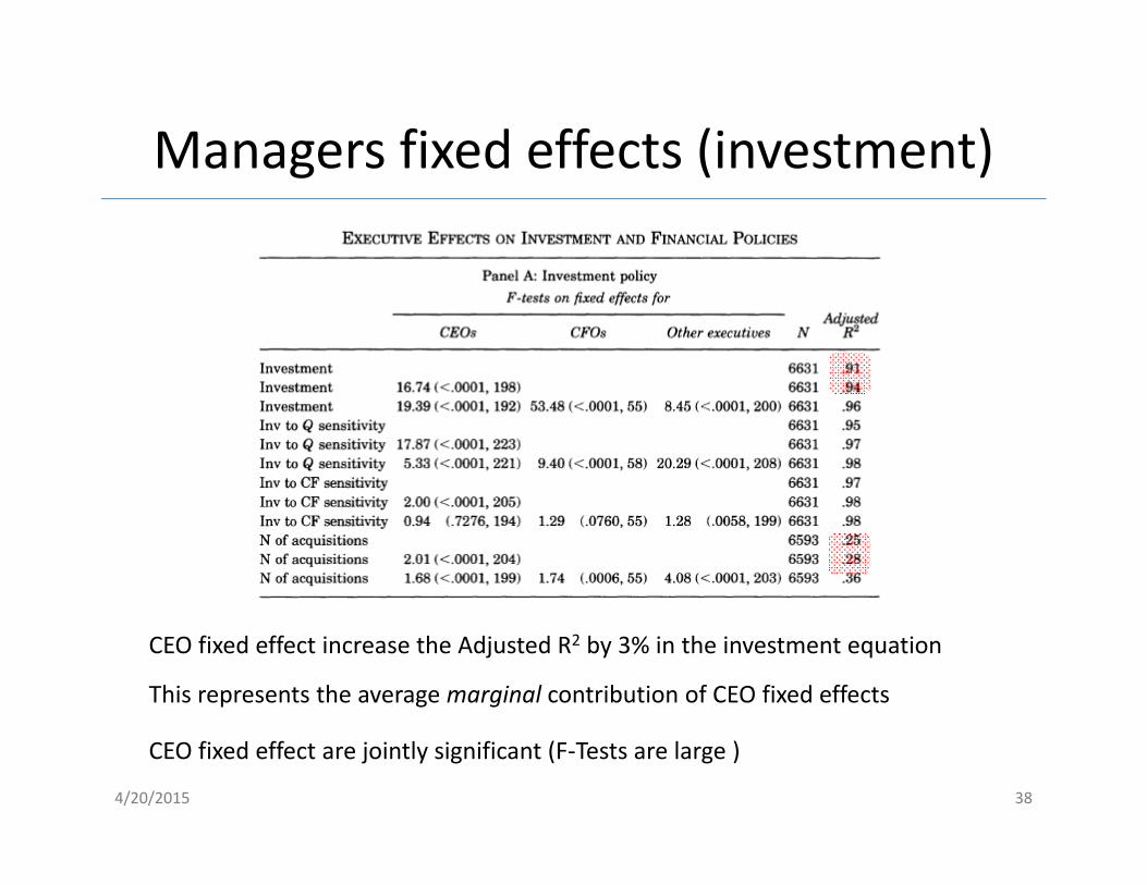
Managers fixed effects (investment)
4/20/2015 38
CEO fixed effect increase the Adjusted R2 by 3% in the investment equation
CEO fixed effect are jointly significant (F‐Tests are large )
This represents the averagemarginal contribution of CEO fixed effects
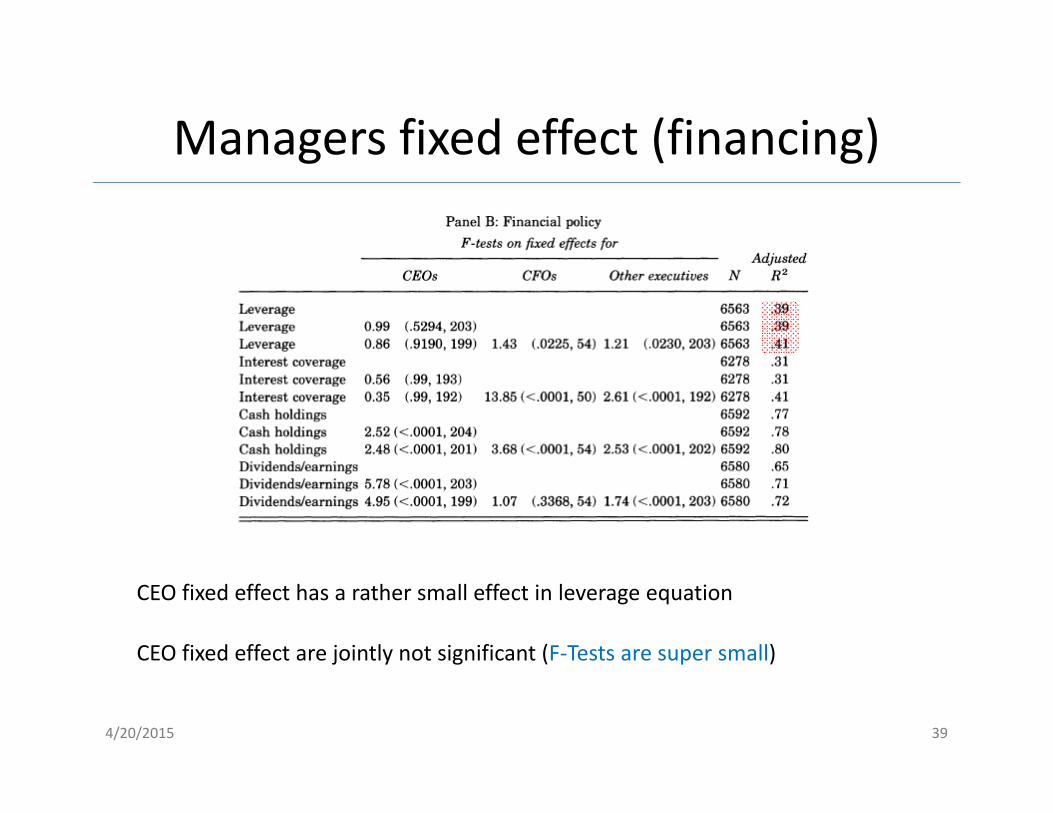
Managers fixed effect (financing)
4/20/2015 39
CEO fixed effect has a rather small effect in leverage equation
CEO fixed effect are jointly not significant (F‐Tests are super small)

Managers fixed effects (performance)
4/20/2015 40
CEO fixed effects are significant in performance equations
Controlling for many different things, some CEOs are related to better performance

Magnitude of the managers fixed effects?
• Retrieve the estimated managers fixed effect from the LSDV estimation (e.g. in Stata)
• Important heterogeneity across managers
4/20/2015 41
Some CEO are negatively related to
performance!

Management styles?• Can we detect systematic « styles » among managers fixed effect? (Use simple OLS
regression)
• We do see consistent patterns (e.g internal vs external investment or debt vs cash)
4/20/2015 42

Fixed effects and compensation
4/20/2015 43
Managers fixed effect appear to be related to theircompensation!
Firms appear to pay a premium for managers who are associated with higher rates of return on assets!
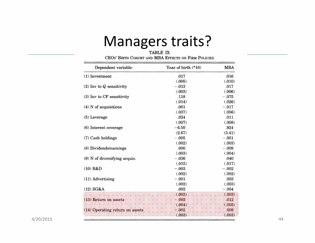
Managers traits?
4/20/2015 Empircal Corporate Finance 44

Conclusion/comments• CEO appear to matter
• CEO Systematically related to corporate policies
• This has generated a lot of research on WHY do CEO matter (some explanations)
– Overconfident CEO
– Connected CEO (political, school, investment bankers, private equity)
– Financial expertise
• Original use of fixed effects to answer an interesting question (not a causalquestion though)
• This type of approach has been used by others in the literature
4/20/2015 45

Think about Standard Errors!
Petersen (2009)
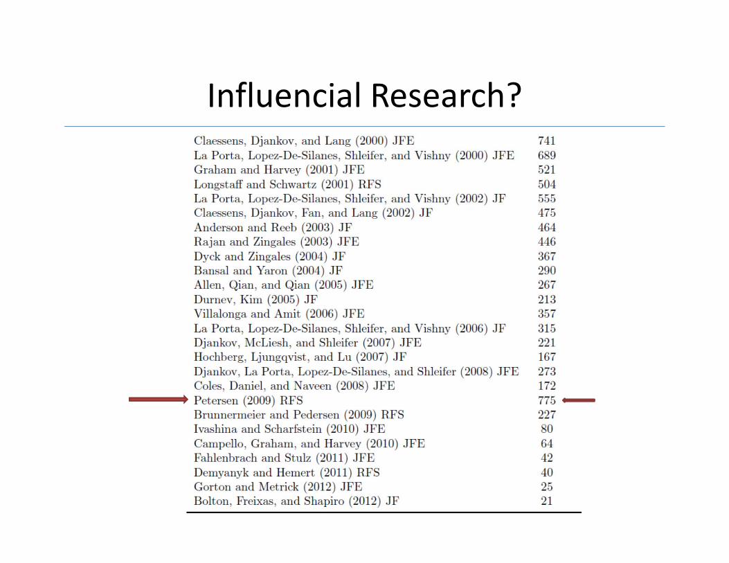
Influencial Research?
Potential Problem?
• In panel data, residuals may be correlated across firms and across time (not iid)
• Why?
• Consequences?– OLS standard errors (hence t‐stats) can be biased– May lead to wrong conclusion
• Let’s see what happens and what can de done
4/20/2015 48

Pooled OLS
• Simple panel model (firm i, time t)
4/20/2015 49
IID
Assume Cov(X, ε)=0
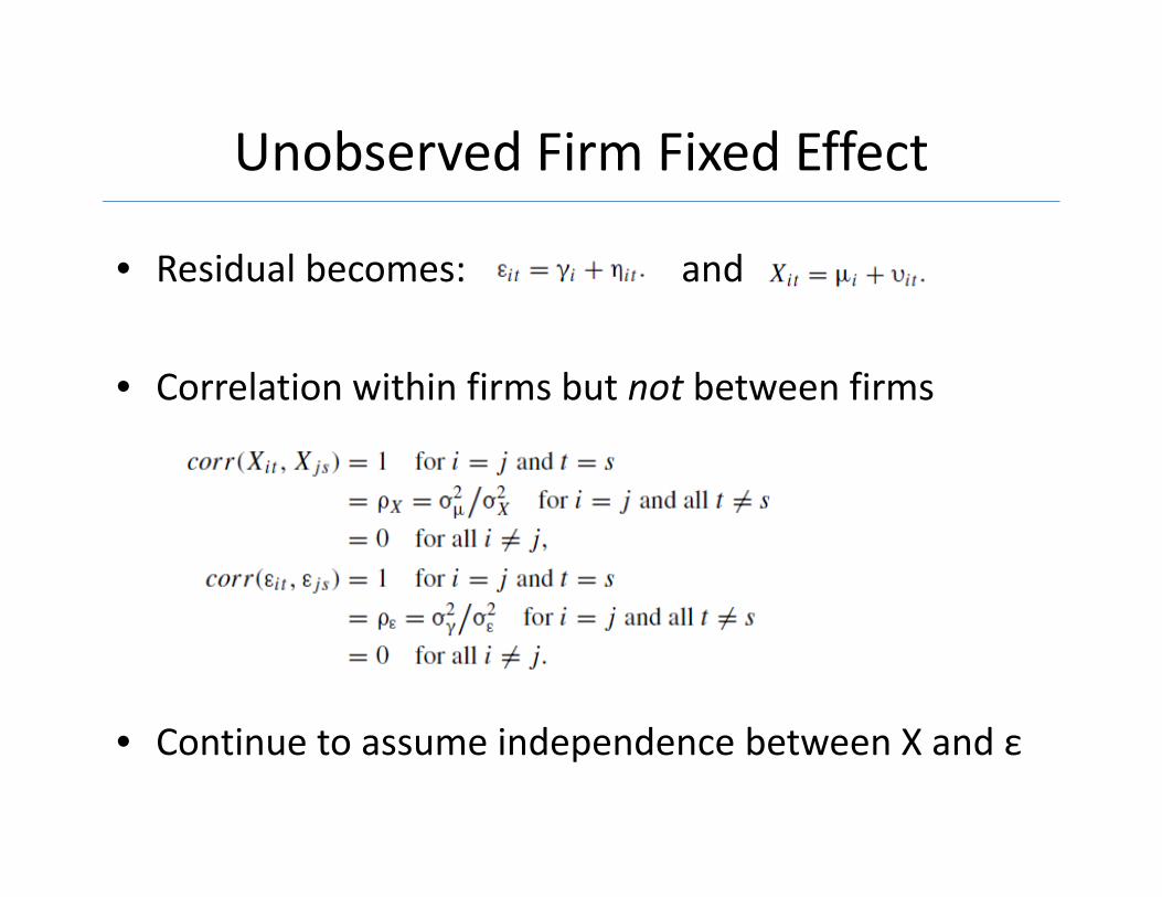
Unobserved Firm Fixed Effect
• Residual becomes: and
• Correlation within firms but not between firms
• Continue to assume independence between X and ε

True Standard Errors (OLS)?
OLS understates true standard errors if ρs are not zero! + Increases in T

True Residual Structure

How bad it this?
• Simulation of a panel dataset with a firm fixed effect
• Repeat this several time to observe “true” SE
• SE of y=1 and SE of ε=2 R2=20%
• Change the fraction of the variance of y that is due to the firm fixed effect (0%‐75%)
• Change the fraction of the variance of ε that is due to the firm fixed effect (0%‐75%)

True SE
OLS SE
OLS SE cluster

Time effect?
• Petersen (2009) execute a similar analysis for
– Time fixed effect (cross‐firm residual correlation)
– Firm and Time fixed effect
– Temporary Firm fixed effect (decay)
• Bottom line: Everything potentially create BIASES

Application: Capital Structure

Take‐Away
• In the presence of firm fixed effect– OLS SE are biased– SE clustered by firm are unbiased
• In the presence of a time fixed effect– OLS SE are biased– Fama‐McBeth SE are unbiased
• In the presence of both– Include time dummies and cluster by firm– Double cluster by time and firm
• Learn about the structure of the data

Stata and SAS code and help
http://www.kellogg.northwestern.edu/faculty/petersen/htm/papers/standarderror.html