Empirical likelihood estimation of the spatial quantile regression

Article

Empirical likelihood estimation of the spatial quantile regression

Kostov, Phillip

Available at http://clok.uclan.ac.uk/3809/

Kostov, Phillip ORCID: 0000-0002-4899-3908 (2012) Empirical likelihood estimation of the spatial quantile regression. Journal of Geographical Systems . ISSN 1435-5930

It is advisable to refer to the publisher’s version if you intend to cite from the work.http://dx.doi.org/10.1007/s10109-012-0162-3

For more information about UCLan’s research in this area go to http://www.uclan.ac.uk/researchgroups/ and search for <name of research Group>.

For information about Research generally at UCLan please go to http://www.uclan.ac.uk/research/

All outputs in CLoK are protected by Intellectual Property Rights law, includingCopyright law. Copyright, IPR and Moral Rights for the works on this site are retainedby the individual authors and/or other copyright owners. Terms and conditions for useof this material are defined in the policies page.

CLoKCentral Lancashire online Knowledgewww.clok.uclan.ac.uk

https://clok.uclan.ac.uk/policies.html

http://www.uclan.ac.uk/research/

http://www.uclan.ac.uk/researchgroups/

This is pre-print of an article published in Journal of Geographical Systems. The final publication is

available at www.springerlink.com or at http://dx.doi.org/10.1007/s10109-012-0162-3

Empirical likelihood estimation of the spatial

quantile regression

Philip Kostov

University of Central Lancashire

Abstract

The spatial quantile regression model is a useful and flexible model for analysis of empirical problems with

spatial dimension. This paper introduces an alternative estimator for this model. The properties of the proposed

estimator are discussed in a comparative perspective with regard to the other available estimators. Simulation

evidence on the small sample properties of the proposed estimator is provided. The proposed estimator is

feasible and preferable when the model contains multiple spatial weighting matrices. Furthermore a version of

the proposed estimator based on the exponentially tilted empirical likelihood could be beneficial if model

misspecification is suspect.

JEL codes: C21, C26

Introduction

Spatial models are quickly gaining prominence in areas such as economics, sociology

environmental studies and economic geography building on a long standing tradition in

regional studies, real estate and geographical analysis. The popularity of such methods is

partially due to the realisation that ‘space’ need not be only geographical, but alternative

distance metrics, such as economic and social distances can be employed instead resulting in

wide applicability of ‘spatial’ analysis methods. As a result whenever one is concerned with

analysis of issues such as social interaction, social norms, social capital, neighbourhood

effects, peer group effects, strategic interaction, reference behaviour or yardstick competition

theoretical models applying to such concepts are very likely to be susceptible to investigation

involving ‘spatial’ methods.

Some examples of theoretical models explicitly considering such issues include the models of

increasing returns, path dependence and imperfect competition that underline much of the

new economic geography literature (see Fujita et al. 1999 for an overview), neighbourhood

spillover effects (Durlauf 1994; Borjas 1995; Glaeser et al. 1996) macroeconomic interaction

models (Aoki 1996 and Durlauf 1997) and the interaction framework of Brueckner (2003).



It is then not surprising that a rich methodological literature dealing with specification,

estimation and testing of spatial models have developed. A wide range of statistical methods

and models have been developed to allow empirical analysis. This paper contributes to this

literature by proposing an alternative estimation method, namely smoothed empirical

likelihood, for the recently introduced spatial quantile regression model. The next section

briefly reviews the spatial quantile regression. Then we outline the empirical likelihood

estimation of the model. The practicalities of the implementation are compared to the

alternative estimation methods in terms of advantages and disadvantages in order to help

researchers with informal guidelines of which methods would be preferable under what

circumstances. Finally we present Monte Carlo study of the finite sample properties of the the

proposed estimator.

Spatial quantile regression

Here we will consider the so called spatial quantile regression model. Since this particular

term has been used to denote two very different specifications it is important to clarify which

one we are referring to. In this paper we follow the definition provided in Kostov (2009).

Recently Reich et al. (2011) proposed a totally different model which they also called spatial

quantile regression. Their model is a quantile regression with Bernstein polynomial basis

representation for the coefficients in which the basis functions are allowed to vary over space.

The model of Reich et al. (2011) is a compromise between (Bayesian) non-parametric and

parametric approaches to the quantile reression problem. The model of Kostov (2009) on the

other hand is fully parametric (frequentist) quantile regression, characterised by endogeneity.

The spatial quantile regression model, proposed by Kostov (2009) reads as:

sy W y X u (1)

It is a straightforward quantile regression extension of the widely used in spatial

econometrics linear spatial lag model. The quantile of the dependent variable y is modeled as

a function of its spatial lag sW y (obtained using some predetermined exogenous spatial

weighting matrix sW ) and explanatory variables X. Hereafter we will treat the spatial

weighting matrix as given. It is worth noting that the latter can be viewed as a combination of

‘spatial’ connectedness (neighbourhood structure) and weighting scheme, and defines an

interaction pattern amongst the units of analysis. Although discussing the way such



interaction pattern is to be determined falls outside the scope of the present paper, the actual

metrics system for doing so does not need to be geographical, as the term ‘spatial’ implicitly

suggests. Indeed wide range of alternative distance metrics, such as economic, social,

technological, cultural etc. can be employed to produce such ‘spatial’ weighting matrices and

the implications of the spillovers represented by these can be analysed by this model.

The same model has been studied in Su and Yang (2011) under the name spatial quantile

autoregression, a name that makes the link to the mean model that is being generalised, much

more explicit. Since in essence the spatial quantile regression is a straightforward

generalization of the (mean) spatial lag model, in empirical analysis similarly to the latter, the

main point of interest will be the partial derivatives 1

sI W

, rather than the raw

coefficients . Hereafter, in order to simplify discussion we will ignore this and will

focus on estimation issues, concerned with the raw coefficients.

In contrast to the standard (linear) spatial lag model the spatial lag parameter and the

vector of regression parameters are -dependent, where is the corresponding

quantile of the dependent variable. There are some distinct advantages that this model offers,

in particular the ability to approximate (monotonic) nonlinear functions by using an estimator

characterised by a parametric rate of convergence (see Kostov, 2009 for more details).

Furthermore since the quantile regression method does not involve any assumptions about the

error term (in this case u), the latter can exhibit arbitrary forms of heteroscedasticity,

including spatial dependence, which in the linear spatial modelling is represented by the so

called spatial error representation. So the spatial quantile regression can easily combine both

spatial lag and spatial error type of dependence in one parsimonious representation. One has

to note that although in general (spatial) dependency in the error term does not affect

estimators’ consistency (which is also valid for quantile regression estimators), it can have a

detrimental effect of efficiency. The latter is however an issue that concerns the construction

of confidence intervals. Even in the standard quantile regression with no endogeneity,

different methods for construction of confidence intervals can be employed, some of which

require stronger assumptions (such as e.g. iid of the errors), while others (e.g. the Monte

Carlo Marginal Bootstrap method) do not. (see Koenker 2005 for an overview).



There is another interesting property of this model. Since this specification allows the spatial

parameter to be dependent on , it can accommodate a different degree of spatial

dependence at different points of the response distribution. For example we could have

spatial lag dependence only present in some parts of the distribution of the dependent

variable, but not in other. Whether one wants to have a varying degree of spatial dependence

or not, depends of course on the particular aims of the analysis and nature of the empirical

problem. Therefore this model may not be suitable for every purpose. Note however that it is

possible in principle to impose certain restrictions to the model, such as for example making

the spatial dependence parameter fixed (i.e. common across quantiles) resulting in a

restricted version of the model represented by Eq. (1). Here however we will ignore such

possibilities and will focus on the original specification for the spatial quantile regression.

Since the spatial lagged variable is present on the right hand side of (1) then, similarly to the

mean case, the conventional quantile regression estimator of Koenker and Bassett (1978) will

in general be inconsistent. To solve the exogeneity problem Kostov (2009) proposed

instrumental quantile regression estimation. In particular two different estimators could be

implemented. The first is the two-stage quantile regression estimator of Kim and Muller

(2004), implemented in a spatial setting by Zietz et al. (2008). The other is the instrumental

variable quantile regression method of Chernozhukov and Hansen (2006), adapted to spatial

models in Kostov (2009). While Kostov (2009) implicitly considers only a spatial lag type of

dependence, Su and Yang (2011) extend the theoretical arguments of Chernozhukov and

Hansen (2006) and prove the applicability of their method under general dependent data

design. The two-stage quantile regression estimator of Kim and Muller (2004) also assumes

i.i.d. data is not applicable to dependent data.

This paper suggests an alternative estimator, namely a smoothed empirical likelihood

estimator for the spatial quantile regression. The next section briefly reviews the empirical

likelihood approach and introduces the estimator. It is then compared to the other alternative

estimators. Then we present simulation evidence of its performance relative to other spatial

estimation methods.



Empirical likelihood estimator

The empirical likelihood (EL) method (Owen 1988, 1990, 1991) is a nonparametric analogue

of likelihood estimation and can be applied to inference of distribution functionals. Its

asymptotic variance is the same as that of the efficient GMM (meaning that it is

asymptotically efficient). The empirical likelihood (EL) estimator is studied in some detail in

Owen (1988), Qin and Lawless (1994) and Imbens (1997). Newey and Smith (2004) showed

that the EL estimator and some other related methods, such as the continuous updating

estimator (CUE) of Hansen et al. (1996), and the exponential tilting (ET) estimator of

Kitamura and Stutzer (1997) and Imbens et al. (1998) all belong to the same family of

generalised empirical likelihood (GEL) estimators (although strictly speaking they extend the

earlier result of Smith (1997) with regard to the EL and ET). Furthermore Newey and Smith

(2004) have proven some interesting theoretical results. These include the fact that in addition

to being robust to the number of moment restrictions, the higher order bias of GEL equals the

asymptotic bias of the infeasible GMM (i.e. the GMM constructed using the optimal

(asymptotic variance minimizing) linear combination).

A major obstacle to the more widespread usage of the above EL type of estimators is the fact

that direct optimisation of their objective function can be numerically complicated. This has

precluded full-blown Monte Carlo studies of their presumably better finite sample properties.

Ramalho (2005) is one of few exceptions with empirical results demonstrating the better

performance of the EL type of estimators over the GMM estimators.

To facilitate the discussion consider the following alternative representation of the spatial

quantile regression model of Kostov (2009):

' 'i i i iy d X u (2)

where for each i= 1,...,n ( where n is the sample size) iy is the dependent variable, iX is a kx1

vector of exogenous covariates, is a kx1 vector of (fixed ) parameters and similarly id

and are correspondingly a sx1 vectors of endogenous variables and their associated

coefficients. In this case the endogeneous variables are simply spatial lags of the dependent

variable i.e. i id W y for some spatial weighting matrix W.

In principle the parameters are varying by quantile and should be indexed by it in Eq. (2)

above. Here however for simplicity we will focus our attention on a single (unspecified)



quantile and for this reason the usual quantile dependence of the model parameters will be

omitted from the notation. We also intentionally use notation indexed by observation in order

to facilitate the expression of the associated estimating functions that we will introduce and

use to specify the empirical likelihood estimator.

Kostov’s (2009) spatial quantile regression model explicitly sets s=1, but we will not impose

this restriction here. In this way our set up fits the more general quantile regression model

with endogenous covariates. Furthermore iu is an (unobserved) error term that satisfies the

usual quantile restriction 0 | ,i i iP u X w , where is the quantile of interest.

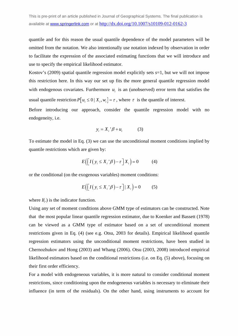
Before introducing our approach, consider the quantile regression model with no

endogeneity, i.e.

'i i iy X u (3)

To estimate the model in Eq. (3) we can use the unconditional moment conditions implied by

quantile restrictions which are given by:

' 0i i iE I y X X (4)

or the conditional (on the exogenous variables) moment conditions:

' | 0i i iE I y X X (5)

where I(.) is the indicator function.

Using any set of moment conditions above GMM type of estimators can be constructed. Note

that the most popular linear quantile regression estimator, due to Koenker and Bassett (1978)

can be viewed as a GMM type of estimator based on a set of unconditional moment

restrictions given in Eq. (4) (see e.g. Otsu, 2003 for details). Empirical likelihood quantile

regression estimators using the unconditional moment restrictions, have been studied in

Chernozhukov and Hong (2003) and Whang (2006). Otsu (2003, 2008) introduced empirical

likelihood estimators based on the conditional restrictions (i.e. on Eq. (5) above), focusing on

their first order efficiency.

For a model with endogeneous variables, it is more natural to consider conditional moment

restrictions, since conditioning upon the endogeneous variables is necessary to eliminate their

influence (in term of the residuals). On the other hand, using instruments to account for



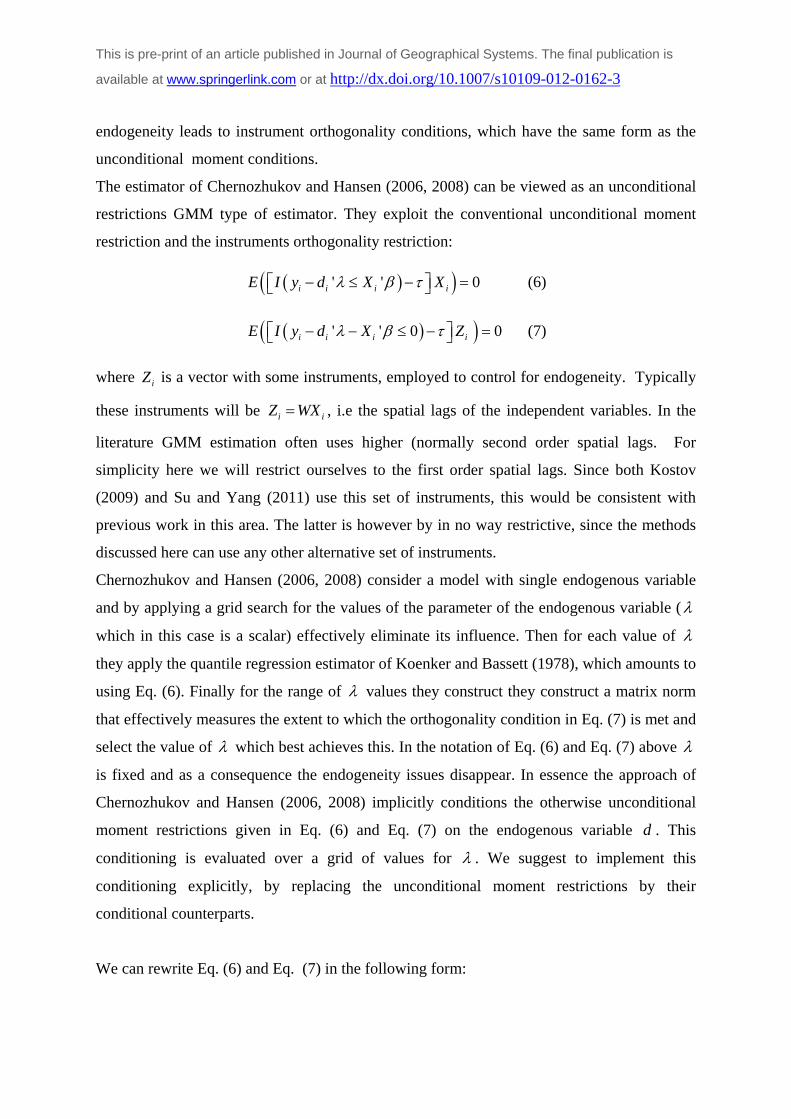
endogeneity leads to instrument orthogonality conditions, which have the same form as the

unconditional moment conditions.

The estimator of Chernozhukov and Hansen (2006, 2008) can be viewed as an unconditional

restrictions GMM type of estimator. They exploit the conventional unconditional moment

restriction and the instruments orthogonality restriction:

' ' 0i i i iE I y d X X (6)

' ' 0 0i i i iE I y d X Z (7)

where iZ is a vector with some instruments, employed to control for endogeneity. Typically

these instruments will be i iZ WX , i.e the spatial lags of the independent variables. In the

literature GMM estimation often uses higher (normally second order spatial lags. For

simplicity here we will restrict ourselves to the first order spatial lags. Since both Kostov

(2009) and Su and Yang (2011) use this set of instruments, this would be consistent with

previous work in this area. The latter is however by in no way restrictive, since the methods

discussed here can use any other alternative set of instruments.

Chernozhukov and Hansen (2006, 2008) consider a model with single endogenous variable

and by applying a grid search for the values of the parameter of the endogenous variable (

which in this case is a scalar) effectively eliminate its influence. Then for each value of

they apply the quantile regression estimator of Koenker and Bassett (1978), which amounts to

using Eq. (6). Finally for the range of values they construct they construct a matrix norm

that effectively measures the extent to which the orthogonality condition in Eq. (7) is met and

select the value of which best achieves this. In the notation of Eq. (6) and Eq. (7) above

is fixed and as a consequence the endogeneity issues disappear. In essence the approach of

Chernozhukov and Hansen (2006, 2008) implicitly conditions the otherwise unconditional

moment restrictions given in Eq. (6) and Eq. (7) on the endogenous variable d . This

conditioning is evaluated over a grid of values for . We suggest to implement this

conditioning explicitly, by replacing the unconditional moment restrictions by their

conditional counterparts.

We can rewrite Eq. (6) and Eq. (7) in the following form:



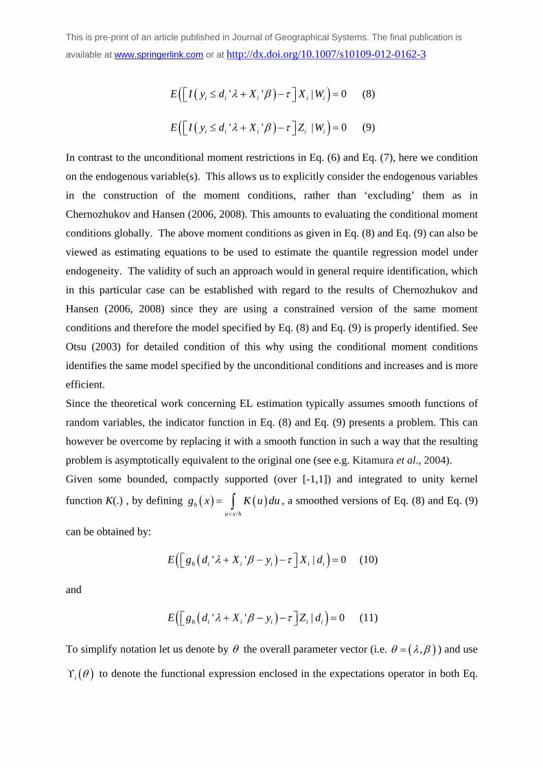
' ' | 0i i i i iE I y d X X W (8)

' ' | 0i i i i iE I y d X Z W (9)

In contrast to the unconditional moment restrictions in Eq. (6) and Eq. (7), here we condition

on the endogenous variable(s). This allows us to explicitly consider the endogenous variables

in the construction of the moment conditions, rather than ‘excluding’ them as in

Chernozhukov and Hansen (2006, 2008). This amounts to evaluating the conditional moment

conditions globally. The above moment conditions as given in Eq. (8) and Eq. (9) can also be

viewed as estimating equations to be used to estimate the quantile regression model under

endogeneity. The validity of such an approach would in general require identification, which

in this particular case can be established with regard to the results of Chernozhukov and

Hansen (2006, 2008) since they are using a constrained version of the same moment

conditions and therefore the model specified by Eq. (8) and Eq. (9) is properly identified. See

Otsu (2003) for detailed condition of this why using the conditional moment conditions

identifies the same model specified by the unconditional conditions and increases and is more

efficient.

Since the theoretical work concerning EL estimation typically assumes smooth functions of

random variables, the indicator function in Eq. (8) and Eq. (9) presents a problem. This can

however be overcome by replacing it with a smooth function in such a way that the resulting

problem is asymptotically equivalent to the original one (see e.g. Kitamura et al., 2004).

Given some bounded, compactly supported (over [-1,1]) and integrated to unity kernel

function K(.) , by defining /

h

u x h

g x K u du

, a smoothed versions of Eq. (8) and Eq. (9)

can be obtained by:

' ' | 0h i i i i iE g d X y X d (10)

and

' ' | 0h i i i i iE g d X y Z d (11)

To simplify notation let us denote by the overall parameter vector (i.e. , ) and use

i to denote the functional expression enclosed in the expectations operator in both Eq.



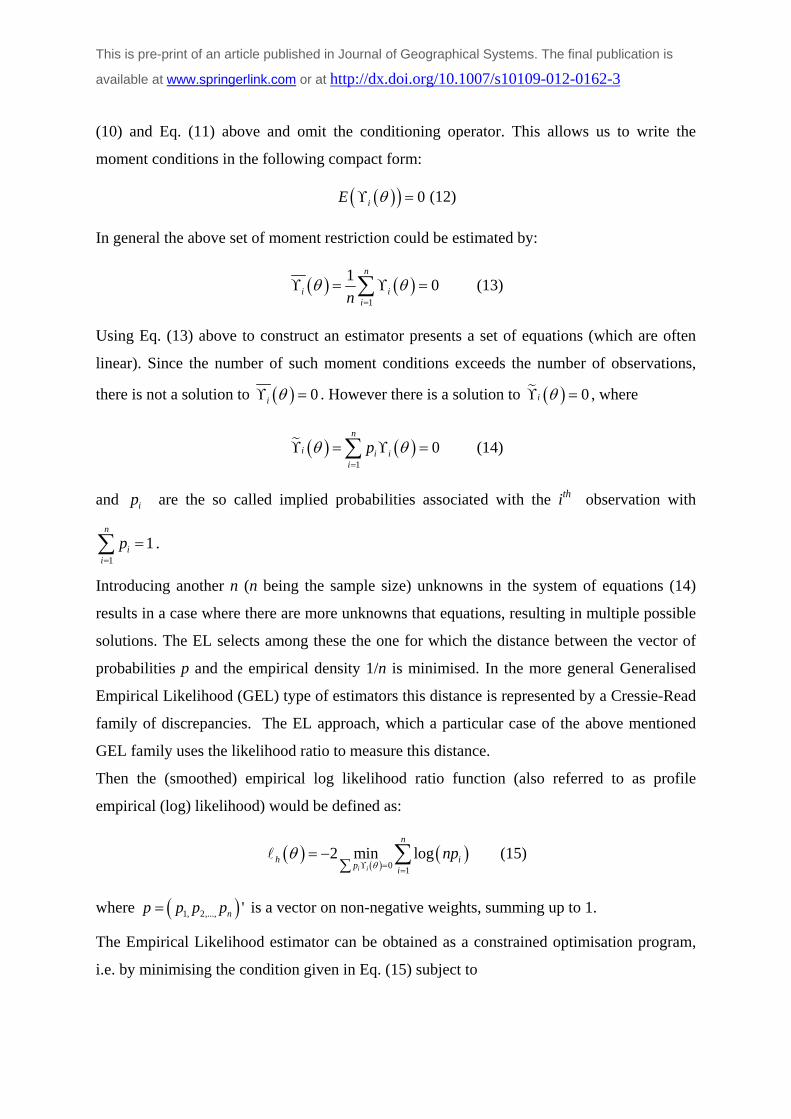
(10) and Eq. (11) above and omit the conditioning operator. This allows us to write the

moment conditions in the following compact form:

0iE (12)

In general the above set of moment restriction could be estimated by:

1

10

n

i iin

(13)

Using Eq. (13) above to construct an estimator presents a set of equations (which are often

linear). Since the number of such moment conditions exceeds the number of observations,

there is not a solution to 0i . However there is a solution to 0i , where

1

0n

i i ii

p

(14)

and ip are the so called implied probabilities associated with the ith observation with

1

1n

ii

p

.

Introducing another n (n being the sample size) unknowns in the system of equations (14)

results in a case where there are more unknowns that equations, resulting in multiple possible

solutions. The EL selects among these the one for which the distance between the vector of

probabilities p and the empirical density 1/n is minimised. In the more general Generalised

Empirical Likelihood (GEL) type of estimators this distance is represented by a Cressie-Read

family of discrepancies. The EL approach, which a particular case of the above mentioned

GEL family uses the likelihood ratio to measure this distance.

Then the (smoothed) empirical log likelihood ratio function (also referred to as profile

empirical (log) likelihood) would be defined as:

0

1

2 min logi i

n

h ip

i

np

(15)

where 1, 2,..., 'np p p p is a vector on non-negative weights, summing up to 1.

The Empirical Likelihood estimator can be obtained as a constrained optimisation program,

i.e. by minimising the condition given in Eq. (15) subject to



1

1n

ii

p

and 1

0n

i ii

p

.

The standard Langrage Multiplier method allows one to derive the optimal weights and

replacing them back into the empirical log likelihood ratio expression one can obtain:

1

2 log 1 'n

h ii

t

(16)

where t is a vector of Lagrange multipliers.

Then the smoothed empirical likelihood estimator can be defined as:

ˆ arg min h (17)

We also need confidence intervals for the smoothed empirical likelihood (SEL) estimates.

Different methods to obtain such confidence intervals are discussed in Whang (2006) and

Otsu (2008). These however rely on explicit assumption of just identification, while the

spatial quantile regression model we consider here is over-identified. Alternatively we could

use a quasi-posterior based on the EL objective function as proposed in Chernozhukov and

Hong (2003) and employ Markov chain methods to derive confidence intervals, in a way

reminiscent of the Bayesian approach to the problem. Strictly speaking Chernozhukov and

Hong (2003) assume i.i.d. data for constructing the appropriate sampler. This assumption can

however be relaxed and their suggested approach is applicable to dependent data. Here

however we will follow the most generally applicable standard approach to obtaining

confidence intervals. Solving Eq. (17) provides us with point estimates for the parameters.

Similarly to the parametric likelihood we can obtain confidence intervals by simply

contouring the empirical likelihood ratio.

Given the point estimates for each parameter we can apply the following to find the

confidence limits at a given confidence level. Here we only describe this for the upper

boundary, but the same algorithm is used to obtain the lower boundary.

(i) Take some starting value for the upper boundary.

(ii) Then estimate a restricted quantile regression model in which the value for this parameter

is fixed at the current upper boundary.

(iii) Calculate the smoothed empirical likelihood ratio for the restricted model with regard to

the full model. Compare with the desired probability level (the ELR follows asymptotically



chi–square distribution, see Owen, 1990). Adjust the value for the upper boundary if

necessary.

Steps (ii)-(iii) are iterated through until the desired probability level is achieved. This

procedure is then repeated for both the upper and lower boundary for each coefficient. In

principle step 2 involves repeatedly solving problems like Eq. (17). One can however greatly

reduce the computational load and use simpler to calculate estimator, such as the linear

programming estimator of Koenker and Bassett (1978) instead in step 2. As for the starting

values, these are not crucial, but values that are closer to the reality will reduce the number of

search iterations. Therefore one may use the standard errors estimates from a conventional

quantile regression routine. Taking into account that the EL intervals can be expected to be

more conservative and therefore wider it would be desirable to increase the starting intervals.

For example while adding (or subtracting for the lower boundary) two standard errors to the

parameter value, could be considered a workable strategy, one may want to increase this to

say 3 standard errors (or 2.5 as in the present application) in order to get closer to the final

results.

Contouring the empirical likelihood ratio however depends on it being (asymptotically) chi–

square distributed. When considering model with dependent data however, although the

empirical likelihood estimates remain consistent, the dependency in the data may cause the

empirical likelihood ratio to lose it chi-square distribution. (see Kitamura, 1997 for details).

Several alternatives to produce confidence intervals could be used. Spatial bootstrap (both

parametric and non-parametric) could be employed, but this would in general be undesirable

due to the high computational costs. Alternatively the block empirical likelihood approach of

Kitamura (1997) can be used.

The blocking idea amounts to treating dependence in a fully nonparametrical way. It is easier

to explain it in the time series setting where it was originally introduced. One uses blocks of

consecutive observations to provide a nonparametric evaluation of the dependence in the

data. The time series blockwise empirical likelihood was first proposed by Kitamura (1997)

and Kitamura and Stutzer (1997). It proceeds as follows. First one forms blocks of

observations. The aim of forming such blocks is to retain the dependence pattern within each

block. At the same time, similarly to the block bootstrap, the dependence structure between

the blocks is destroyed. Then one simply applies the ‘standard’ EL estimation treating the

block as if they were i.i.d. observations. The only difference is that the moment conditions

i.e. Eq. (10) and Eq. (11) in our representation) are replaced by what Kitamura and Stutzer



(1997) call the ‘smoothed moment function’, which is simply the averaged over each block

moment function. Kitamura (1997) suggests that more general weighting schemes (in place

of simple averaging) could be employed but virtually all related research uses averaging.

The block empirical likelihood estimator has been shown to achieve the same asymptotic

efficiency as an optimally weighted GMM for the dependent data case (see Kitamura, 1997

for details). Although the standard and the block empirical likelihood are both consistent and

can be used for obtaining point estimates, in the case of weakly dependent data the block EL

can be used to provide valid confidence intervals. For weakly dependent quantiles, Chen and

Wong (2009) provide theoretical and simulation evidence for the performance of the block

empirical likelihood. They also suggest data dependent smoothing to better capture the

dependency pattern. Their results are directly relevant in this case since the restriction on the

dependency present in the data, namely alpha mixing is the same as the one assumed in Su

and Yang (2011).

Note however that here we deal with spatial data. Since the latter is typically characterised by

two dimensions, constructing blocks of data that preserve spatial dependence is slightly more

involved than in the time series case. Nordman (2008) provides detailed account for block

sampling schemes for spatial empirical likelihood for lattice data. These schemes are

essentially the same as these used in the spatial block bootstrap and spatial subsampling (see

Lahiri, 2003 for a detailed overview of the latter). In essence this requires resampling

rectangular blocks of data. The size of these blocks has to be large enough to capture any

spatial dependence, but for theoretical reasons should increase more slowly than the sample

size. The optimal size of the blocks is an open issue and it often depends on the purpose of

the estimation. Probably the most popular method for selecting the block size is the so called

‘minimum volatility’ method, of Politis et al. (1999, see section 9.3.2). It is a heuristic based

on the premise that although some block sizes could be too small or too large, one may

expect a whole range of values for the block size to yield an asymptotically correct inference.

This is translated into visual inspection of the EL confidence intervals for a range of block

sizes to establish a stability region.

The EL estimation proposed here will be valid under the same set of assumptions as in Su

and Yang (2011). One important difference is that the method suggested here depends on

instrument identification (i.e. their assumption 4(iii)), while for the IVQR this assumption is

not necessary, because under weak identification the method is still valid, and efficient

inference can be obtained by inverting the Wald type statistic, as suggested in Chernozhukov



and Hansen (2008). The cost of dispensing of the above assumption is that the alternative

approach will produce wider confidence intervals (see Kostov 2009 for an empirical

illustration of this point). For the EL approach outlined here however instrument validity is

crucial.

Comparison with alternative estimators

Kim and Muller’s (2004) two–step estimator is by any means computationally simpler than

the other two approaches. It only requires two consecutive quantile regressions. The method

employed in Kostov (2009) and Su and Yang (2011) carries out a search over a set of values

for the spatial lag parameter and thus requires a separate quantile regression to be estimated

for each value in this range. This puts additional computational load on it. The SEL

advocated here requires non-trivial optimisation and hence will in general be computationally

expensive.

The three methods have a totally different approach to controlling for endogeneity. Using the

terminology of Blundell and Powell (2003), the two stage quantile regression (2SQR) uses

the so called ‘fitted values’ approach, replacing the dependent variable and the endogenous

spatially lagged dependent variable by the fitted values from the first stage. The other two

methods employed here, on the other hand can be viewed as estimating functions approaches

(or ‘instrumental variables’ approaches in the terminology of Blundell and Powell, 2003).

The latter two approaches seek to actively impose the orthogonality conditions for the

instruments. In the case of weak identification for example, this would be preferable. In the

latter case for the instrumental quantile regression estimator (IVQR) the indirect approach of

Chernozhukov and Hansen (2008) based on inverting the Wald test statistic could be

employed to ensure valid finite sample inference as demonstrated in Kostov (2009). For the

SEL estimator, the general EL higher order asymptotic efficiency arguments apply leading to

better finite sample performance, although inference is dependent on the right choice of block

size. It is worth mentioning that there is a third approach to endogeneity, namely the ‘control

function’ (CF) approach. For a (non-spatial) quantile regression application of the latter, see

Lee (2007).

In the 2SQR and CF approaches, it is required that a reduced-form equation of the

endogenous variable (used to produce correspondingly the ‘fitted values’ and the ‘control

variable’) is valid, and the estimation of the reduced-from equation is consistent. Then the



asymptotic distributions of the 2SQR and CF estimators will depend on the method used in

the estimation of reduced-form equation of the endogenous variable. In contrast, the

instrumental variable estimators (such as the IVQR or the ELQR) are robust to the method of

obtaining the estimated instrument. They do not require reduced-form equation of the

endogenous variable. In the homoscedastic case all the above estimators could be used to

provide consistent estimates. Under heterogeneous effects however the 2SQR estimates could

be biased (see Chernozhukov and Hansen, 2006 for the theoretical argument and Kwak, 2010

for simulation evidence). Since in the spatial quantile regression the potential spatial

dependence in the data could create such heterogeneity and the conditions under which the

2SQR remains consistent under such circumstances (e.g. constant effect of the endogeneous

variable(s) across quantiles) are rather restrictive, we will not pursue the 2SQR in this paper.

Of course a quantile regression model with constant spatial lag effect could in some

circumstances be a desirable approach, but the model pursued here is much more general.

Another point to consider is the number of endogenous (spatially lagged in this case)

variables. The method used in Kostov (2009) is designed to deal with a single spatially

lagged variable. For more than one endogenous variable a multidimensional grid search will

be required and the latter could be prohibitively expensive from a computational point of

view. It can still be feasible if the simulation methods of Chernozhukov and Hong (2003) are

used to evaluate the objective function (instead of grid search). Since the latter methods can

also be used to evaluate the smoothed empirical likelihood (see the confidence intervals

discussion in previous section) this provides an interesting estimation alternative applicable

for both estimators.

The 2SQR, the CF approach and the SEL on the other hand can deal with an arbitrary number

of endogenous variables. In the spatial context, models with several spatial weighting

matrices can arise naturally, see e.g. LeSage and Fischer (2012) where different ‘spatial’

weighting matrices account for static and dynamic spillovers. Larger number of endogeneous

variables will increase the number of moment conditions to be included in the SEL objective

function hence increasing the computational costs. The largest computational cost to the SEL

estimator however comes from the sample size. Since one needs to evaluate multiple

smoothed quantile score functions, such an evaluation could be computationally demanding

when large samples are employed. Note however, that the explicit motivation of the Kostov’s

(2009) original proposal is obtaining a flexible model with small sample sizes. In the light of



this non-parametric modelling alternative may be preferable for problems with larger sample

sizes.

The SEL proposed here could be further improved by employing Barlett type corrections

and/or bootstrap. Furthermore some more general GEL or pseudo-empirical likelihood

methods could be implemented to the same problem. In particular the robust to

misspecification Exponentially Tilted Empirical Likelihood (ETEL) method of Schennach

(2007) could be of potential interest. The later was originally proposed from a Bayesian point

of view (Schennach, 2005) and an adaptation for quantile regression has been implemented in

Lancaster and Jun (2010) showing promising potential. An interesting potential advantage of

EL methods with many spatially lagged variables is that EL ratio tests could be designed or

the general over-identification tests could be adapted to test the significance of a subset of

spatially lagged variables, providing means for endogenous variables selection. The latter

would of course only be feasible when the number of such variables is relatively small,

because of the potentially considerable computational costs.

Simulation study

In order to investigate the finite sample performance of the proposed estimator, we carried

out a small simulation study. In this study we consider the direct estimates of Eq. (1). Note

that in real word problems analysis correct interpretation of the model parameters would

require computation of the partial derivatives, as suggested in LeSage and Fischer (2008). For

the spatial quantile regression such a computation can be done similarly to the linear spatial

lag model. In order to simplify matters here we will treat these partial derivatives as

unknown.

In principle we follow the simulation design of Su and Yang (2011) with some modifications.

In addition to the empirical likelihood estimator we considered the instrumental variable

quantile regression estimator of Chernozhukov and Hansen (2006, 2008) as well as the

exponentially tilted empirical likelihood (ETEL) estimator of Schennach (2007), adapted to

quantile regression in the same way as the proposed estimator. Since the ETEL estimator is in

principle robust to misspecification, it would be interesting to look at its finite sample

performance for the spatial model. Although in the simulation design we do not consider

misspecification, it is nevertheless useful to consider the cost that such robust estimators pay

whenever misspecification is absent. Additionally we also consider two mean estimator,



namely the spatial two-stage least squares (STSLS) of Kelejian and Prucha (1998) and the

(quasi) Maximum Likelihood (QML) estimator.

The STSLS is probably the simplest, least computationally expensive estimator for spatial lag

type of models, while the QML is still the most widely applicable such estimator.

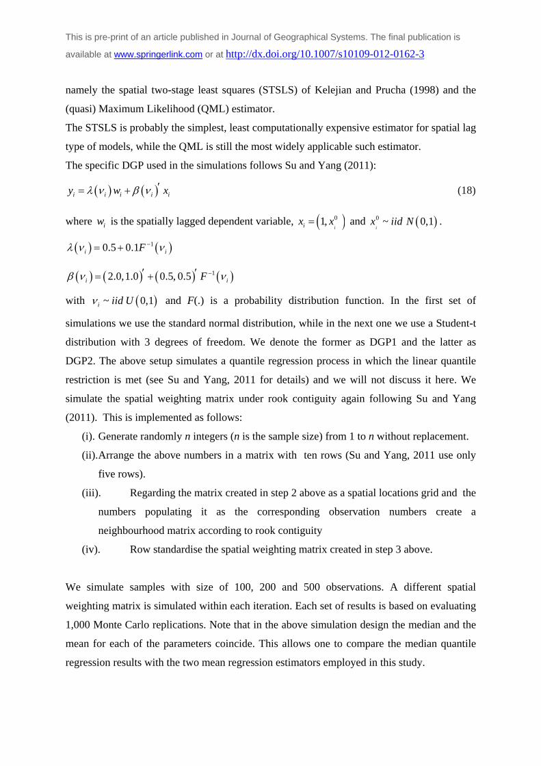
The specific DGP used in the simulations follows Su and Yang (2011):

i i i i iy w x (18)

where iw is the spatially lagged dependent variable, 01,iix x and 0 ~ 0,1

ix iid N .

10.5 0.1i iF

12.0,1.0 0.5, 0.5i iF

with ~ 0,1i iid U and F(.) is a probability distribution function. In the first set of

simulations we use the standard normal distribution, while in the next one we use a Student-t

distribution with 3 degrees of freedom. We denote the former as DGP1 and the latter as

DGP2. The above setup simulates a quantile regression process in which the linear quantile

restriction is met (see Su and Yang, 2011 for details) and we will not discuss it here. We

simulate the spatial weighting matrix under rook contiguity again following Su and Yang

(2011). This is implemented as follows:

(i). Generate randomly n integers (n is the sample size) from 1 to n without replacement.

(ii). Arrange the above numbers in a matrix with ten rows (Su and Yang, 2011 use only

five rows).

(iii). Regarding the matrix created in step 2 above as a spatial locations grid and the

numbers populating it as the corresponding observation numbers create a

neighbourhood matrix according to rook contiguity

(iv). Row standardise the spatial weighting matrix created in step 3 above.

We simulate samples with size of 100, 200 and 500 observations. A different spatial

weighting matrix is simulated within each iteration. Each set of results is based on evaluating

1,000 Monte Carlo replications. Note that in the above simulation design the median and the

mean for each of the parameters coincide. This allows one to compare the median quantile

regression results with the two mean regression estimators employed in this study.



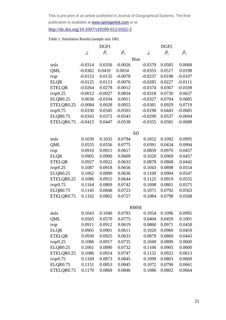
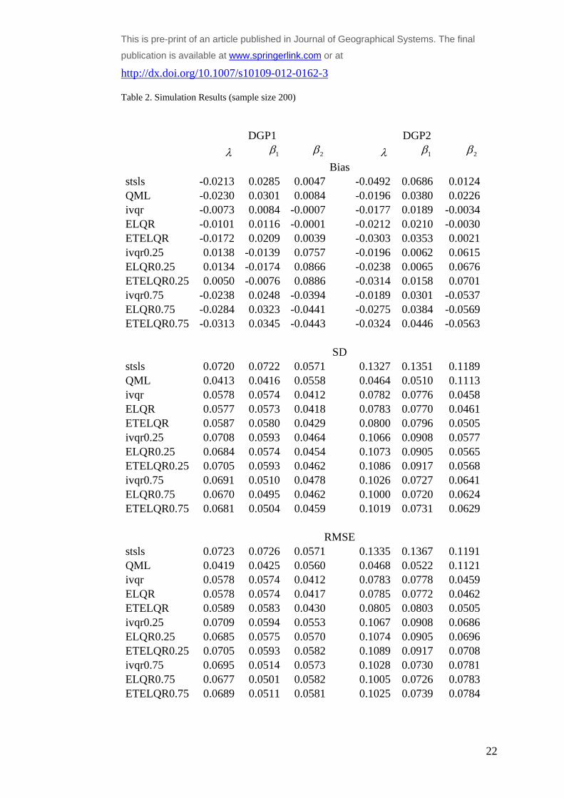
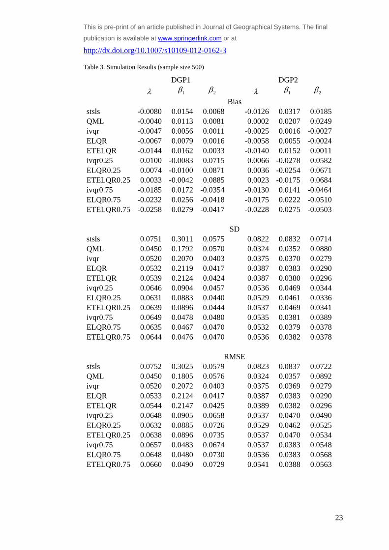
Tables 1-3 present the empirical (i.e. Monte Carlo) bias together with the standard deviation

and the root mean squared errors (RMSE) for each of the compared estimators at the 0.5th ,

0.25th and the 0.75th quantile. Where an estimator is applied to a quantile different from the

median, the acual quantile is added to its description (i.e. ELQR0.25 refers to the EL

estimator applied to the 0.25th quantile). For reporting purposes we standardise the empirical

bias by dividing it by the true value of the corresponding parameters. This allows for direct

comparison of the results across different parameters. The standard deviation and the RMSE

are calculated from the standardised bias and as such are also directly comparable.

Simulation Results

Following similar simulation design to that of Su and Yang (2011) allows for comparison

with their results. The results presented here seem to show slightly higher empirical bias, as

well as standard deviation and RMSE. This is due to on the one hand the slightly different

design for the rook contiguity matrix with ten rather than five rows, which results in a slightly

‘denser’ interaction pattern. The other reason (the random number generation

notwithstanding) for such differences could be the fact that we simulate different spatial

weighting matrix in each iteration. (Su and Yang (2011) are unclear about whether they use

the same spatial weighting matrix in their replications). In general the RMSE decreases

across all estimators, as the sample size increases, which is to be expected.

The first point of interest is the comparative performance of the EL type of estimators for the

0.5th quantile with regard to the conventional mean regression estimators. Although, the

median-based quantile estimators generally perform better than the mean regression

estimator, interestingly they are more dispersed (higher standard deviation and RMSE) than

the QML for the small sample size (n=100). The additional variability introduced by

simulating different spatial weighting matrices could have contributed to such a slower

convergence when the sample size is smaller. The overriding conclusion from this

comparison is that the quantile estimation methods are comparable to the mean regression

method for spatial lag models.

The other, more important issue, to consider is the relative performance of the suggested

estimator against the IVQR at different quantiles. In general the EL estimator performs very

similarly to the IVQR in terms of both bias and RMSE. The ETEL estimators seems to be

slightly worse than the EL one in terms of empirical bias, but tends to perform slightly better



in terms of RMSE under non-normal heteroscedastic errors (i.e. DGP2). This suggests that in

some cases the additional computational costs associated with EL estimators may not bring in

sufficient advantages to justify their usage over the IVQR estimator. Yet, as already

discussed, whenever the IVQR is difficult to implement, as e.g. in models with multiple

spatial weighting matrices, it is preferable, and given that it has similar properties to the

IVQR estimator, it can be a more effective alternative.

Another interesting conclusion from the simulation results, that may require further

investigation is the fact that although being outperformed by the other quantile estimators, the

ETEL estimator is still performing reasonably well. Given that it is robust with regard to

misspecification, it looks like that it pays a relatively small price for such robustness. It could

therefore be interesting to consider the issue of misspecification and the comparable

performance of the alternative estimators in such circumstances. We can nevertheless

tentatively suggest the when a misspecification is suspect, it might be warranted to undertake

ETEL estimation, i.e. to consider the additional computational costs as a trade-off for limiting

its implications on the results. The exact consequences of such a choice will need to be

investigated separately and is beyond the scope of the present study.

Conclusions

This paper suggested an alternative smoothed empirical likelihood estimator for the spatial

quantile regression model. Although this estimator can be computationally demanding for

larger sample sizes, it is feasible and practical for small and medium size samples typical for

spatial dependence problems, where the parametric rate of convergence of the quantile

regression estimators can be most beneficial. The main computational cost of the proposed

procedure lies in contouring the empirical likelihood in order to obtain confidence intervals.

Therefore alternative methods for achieving this task, outlined in the methodology section,

could reduce its computational costs and increase its appeal.

One of the main advantages of our proposal however lies in establishing a general estimation

framework in which the empirical likelihood can be substituted by alternative estimation

criteria (most notably those of the generalised empirical likelihood family) resulting in a

range of estimators that should be able to achieve higher order improvements compared to

more standard (generalised) method of moments approaches.



An added benefit of the proposed method is the ability to handle multiple spatial weighting

matrices, which is difficult for the IVQR methods. Furthermore the simulation evidence

suggests that the ETEL version of the estimator, pays relatively small price (in terms of

efficiency) for allowing for potential misspecification. Although the latter requires further

investigation, it tentatively suggests that this could be a preferred estimation option in

empirical investigations when there are doubts about the correct model specification.

References:

Aoki M. (1996) New Approaches to Macroeconomic Modelling (Cambridge University Press, Cambridge).

Borjas, G J, (1995) Ethnicity, neighborhoods, and human-capital externalities, American Economic Review, 86

(3), 365–390.

Brueckner J K, (2003) Strategic interaction among governments: an overview of empirical studies, International

Regional Science Review, 26 (2) 175-188.

Chen, S X and C. M. Wong (2009), Smoothed block empirical likelihood for quantiles of weakly dependent

processes, Statistica Sinica 19(1), 71-81.

Chernozhukov V, Hansen C. (2006). Instrumental quantile regression inference for structural and treatment

effect models. Journal of Econometrics 132(2): 491–525.

Chernozhukov, V., Hong, H., (2003). An MCMC approach to classical estimation. Journal of Econometrics 115

(2), 293–346.

Chernozhukov,V. and C. Hansen (2008) Instrumental variable quantile regression: A robust inference approach,

Journal of Econometrics 142 (1) , 379–398.

Durlauf S N (1994) Spillovers, stratification and inequality, European Economic Review 38 (3-4), 836–845.

Durlauf S N (1997) Statistical mechanics approaches to socioeconomic behaviour, in The Economy as an

Evolving Complex System II, Eds B W Arthur, S N Durlauf and D A Lane (Addison-Wesley, Reading, MA) pp.

81–104.

Fujita M, Krugman P and Venables A, (1999) The Spatial Economy: Cities, Regions and International Trade

(MIT Press, Cambridge, MA)

Glaeser E L, Sacerdote B and Scheinkman J, (1996) Crime and social interactions, Quarterly Journal of

Economics, 111(2), 507–548.

Hansen, L.P., J. Heaton and A. Yaron (1996). Finite sample properties of some alternative GMM estimators.

Journal of Business and Economic Statistics, 14(3), 262-280.

Imbens, G W (1997). One-step estimators for over-identified generalized method of moments Models, Review of

Economic Studies, 64(3), 359-83.

Imbens, G W, R. H. Spady and P. Johnson (1998). Information theoretic approaches to inference in moment

condition models, Econometrica, 66(2), 333-358.

Kelejian, H.H. and I.R. Prucha. (1998) A generalized spatial two stage least squares procedure for estimating a

spatial autoregressive model with autoregressive disturbances, Journal of Real Estate Finance and Economics

17(1), 99-121.



Kim, T. H. and C. Muller (2004). Two-stage quantile regression when the first stage is based on quantile

regression, Econometrics Journal, 7(1), 218-231.

Kitamura, Y. (1997) Empirical likelihood methods with weakly dependent processes, Annals of Statistics, 25(5),

2084–2102.

Kitamura, Y. and M. Stutzer (1997). An information-theoretic alternative to generalized method of moments

estimation. Econometrica, 65(5), 861-874.

Kitamura, Y., Tripathi, G., Ahn, H., (2004). Empirical likelihood-based inference in conditional moment

restriction models, Econometrica 72(6), 1667–1714.

Koenker, R. (2005) Quantile Regression, Econometric Society Monograph Series, Cambridge University Press.

Koenker, R., Bassett, G., (1978). Regression quantiles. Econometrica 46, 33–50.

Kostov, P. (2009) A spatial quantile regression hedonic model of agricultural land prices, Spatial Economic

Analysis, 4(1), 53-72.

Kwak, D. (2010). Implementation of instrumental variable quantile regression (IVQR) methods. Working Paper,

Michigan State University.

Lahiri, S. N. (2003). Resampling Methods for Dependent Data, Springer Series in Statistics, Springer, London.

Lancaster, T and S. J. Jun (2010) Bayesian quantile regression methods, Journal of Applied Econometrics, 25

(2), 287-307.

Lee, S (2007) Endogeneity in quantile regression models: A control function approach. Journal of

Econometrics, 141 (2) 1131 – 1158.

LeSage J. P. and M. M Fischer (2012) Estimates of the impact of static and dynamic knowledge spillovers on

regional factor productivity, International Regional Science Review 35(1), 103-127.

LeSage J. P. and M. M Fischer (2008) Spatial growth regressions: Model specification, estimation and

interpretation, Spatial Economic Analysis 3(3): 275-304.

Newey,W.K. and R.J. Smith, (2004). Higher order properties of GMM and generalized empirical likelihood

estimators. Econometrica, 72(1), 219-255.

Nordman, D. J. (2008) A blockwise empirical likelihood for spatial lattice data, Statistica Sinica, 18(3), 1111-

1129.

Otsu, T (2003) Empirical likelihood for quantile regression, Manuscript, Department of Economics, University

of Wisconsin.

Otsu, T (2008) Conditional empirical likelihood estimation and inference for quantile regression models,

Journal of Econometrics 142(1), 508–538.

Owen, A. (1988). Empirical likelihood ratio confidence intervals for a single functional. Biometrika, 75 (2),

237–249.

Owen, A. (1990). Empirical likelihood ratio confidence regions. Annals of Statistics, 18 (1), 90–120.

Owen, A. (1991). Empirical likelihood for linear models. Annals of Statistics, 19 (4), 1725–1747.

Pace, R. K. and R. Barry. (1997) Quick computation of spatial autoregressive estimators, Geographical

Analysis, 29 (3), 232-247.

This is pre-print of an article published in Journal of Geographical Systems. The final

publication is available at www.springerlink.com or at

http://dx.doi.org/10.1007/s10109-012-0162-3

21

Table 1. Simulation Results (sample size 100)

DGP1 DGP2

1 2 1 2

Bias stsls -0.0314 0.0356 -0.0026 -0.0379 0.0585 0.0068QML -0.0362 0.0410 0.0054 -0.0355 0.0517 0.0198ivqr -0.0153 0.0135 -0.0078 -0.0237 0.0198 -0.0107ELQR -0.0125 0.0113 -0.0076 -0.0285 0.0227 -0.0111ETELQR -0.0264 0.0278 -0.0012 -0.0374 0.0367 -0.0108ivqr0.25 -0.0012 -0.0027 0.0834 -0.0318 0.0730 0.0637ELQR0.25 0.0036 -0.0104 0.0911 -0.0327 0.0704 0.0685ETELQR0.25 -0.0084 0.0028 0.0955 -0.0381 0.0929 0.0719ivqr0.75 -0.0330 0.0345 -0.0503 -0.0198 0.0443 -0.0685ELQR0.75 -0.0343 0.0372 -0.0543 -0.0290 0.0537 -0.0694ETELQR0.75 -0.0415 0.0447 -0.0538 -0.0355 0.0581 -0.0688

SD stsls 0.1039 0.1035 0.0794 0.1052 0.1092 0.0995QML 0.0555 0.0556 0.0775 0.0391 0.0434 0.0994ivqr 0.0910 0.0911 0.0617 0.0859 0.0970 0.0457ELQR 0.0905 0.0900 0.0609 0.1020 0.0969 0.0457ETELQR 0.0927 0.0922 0.0633 0.0878 0.0868 0.0442ivqr0.25 0.1087 0.0918 0.0656 0.1043 0.0898 0.0554ELQR0.25 0.1062 0.0890 0.0636 0.1100 0.0904 0.0547ETELQR0.25 0.1086 0.0915 0.0644 0.1125 0.0919 0.0555ivqr0.75 0.1164 0.0869 0.0742 0.1098 0.0801 0.0575ELQR0.75 0.1145 0.0848 0.0723 0.1071 0.0792 0.0563ETELQR0.75 0.1162 0.0862 0.0727 0.1084 0.0798 0.0568

RMSE stsls 0.1043 0.1040 0.0793 0.1054 0.1096 0.0995QML 0.0565 0.0570 0.0775 0.0404 0.0459 0.1001ivqr 0.0911 0.0912 0.0619 0.0860 0.0971 0.0458ELQR 0.0905 0.0901 0.0611 0.1020 0.0969 0.0459ETELQR 0.0930 0.0925 0.0633 0.0879 0.0869 0.0443ivqr0.25 0.1086 0.0917 0.0735 0.1049 0.0899 0.0600ELQR0.25 0.1061 0.0890 0.0732 0.1106 0.0905 0.0600ETELQR0.25 0.1086 0.0914 0.0747 0.1132 0.0922 0.0613ivqr0.75 0.1169 0.0873 0.0845 0.1099 0.0803 0.0669ELQR0.75 0.1151 0.0853 0.0845 0.1072 0.0796 0.0661ETELQR0.75 0.1170 0.0869 0.0846 0.1086 0.0802 0.0664



http://dx.doi.org/10.1007/s10109-012-0162-3

22


DGP1 DGP2

1 2 1 2 Bias stsls -0.0213 0.0285 0.0047 -0.0492 0.0686 0.0124QML -0.0230 0.0301 0.0084 -0.0196 0.0380 0.0226ivqr -0.0073 0.0084 -0.0007 -0.0177 0.0189 -0.0034ELQR -0.0101 0.0116 -0.0001 -0.0212 0.0210 -0.0030ETELQR -0.0172 0.0209 0.0039 -0.0303 0.0353 0.0021ivqr0.25 0.0138 -0.0139 0.0757 -0.0196 0.0062 0.0615ELQR0.25 0.0134 -0.0174 0.0866 -0.0238 0.0065 0.0676ETELQR0.25 0.0050 -0.0076 0.0886 -0.0314 0.0158 0.0701ivqr0.75 -0.0238 0.0248 -0.0394 -0.0189 0.0301 -0.0537ELQR0.75 -0.0284 0.0323 -0.0441 -0.0275 0.0384 -0.0569ETELQR0.75 -0.0313 0.0345 -0.0443 -0.0324 0.0446 -0.0563 SD stsls 0.0720 0.0722 0.0571 0.1327 0.1351 0.1189QML 0.0413 0.0416 0.0558 0.0464 0.0510 0.1113ivqr 0.0578 0.0574 0.0412 0.0782 0.0776 0.0458ELQR 0.0577 0.0573 0.0418 0.0783 0.0770 0.0461ETELQR 0.0587 0.0580 0.0429 0.0800 0.0796 0.0505ivqr0.25 0.0708 0.0593 0.0464 0.1066 0.0908 0.0577ELQR0.25 0.0684 0.0574 0.0454 0.1073 0.0905 0.0565ETELQR0.25 0.0705 0.0593 0.0462 0.1086 0.0917 0.0568ivqr0.75 0.0691 0.0510 0.0478 0.1026 0.0727 0.0641ELQR0.75 0.0670 0.0495 0.0462 0.1000 0.0720 0.0624ETELQR0.75 0.0681 0.0504 0.0459 0.1019 0.0731 0.0629 RMSE stsls 0.0723 0.0726 0.0571 0.1335 0.1367 0.1191QML 0.0419 0.0425 0.0560 0.0468 0.0522 0.1121ivqr 0.0578 0.0574 0.0412 0.0783 0.0778 0.0459ELQR 0.0578 0.0574 0.0417 0.0785 0.0772 0.0462ETELQR 0.0589 0.0583 0.0430 0.0805 0.0803 0.0505ivqr0.25 0.0709 0.0594 0.0553 0.1067 0.0908 0.0686ELQR0.25 0.0685 0.0575 0.0570 0.1074 0.0905 0.0696ETELQR0.25 0.0705 0.0593 0.0582 0.1089 0.0917 0.0708ivqr0.75 0.0695 0.0514 0.0573 0.1028 0.0730 0.0781ELQR0.75 0.0677 0.0501 0.0582 0.1005 0.0726 0.0783ETELQR0.75 0.0689 0.0511 0.0581 0.1025 0.0739 0.0784



http://dx.doi.org/10.1007/s10109-012-0162-3

23


DGP1 DGP2

1 2 1 2

Bias stsls -0.0080 0.0154 0.0068 -0.0126 0.0317 0.0185QML -0.0040 0.0113 0.0081 0.0002 0.0207 0.0249ivqr -0.0047 0.0056 0.0011 -0.0025 0.0016 -0.0027ELQR -0.0067 0.0079 0.0016 -0.0058 0.0055 -0.0024ETELQR -0.0144 0.0162 0.0033 -0.0140 0.0152 0.0011ivqr0.25 0.0100 -0.0083 0.0715 0.0066 -0.0278 0.0582ELQR0.25 0.0074 -0.0100 0.0871 0.0036 -0.0254 0.0671ETELQR0.25 0.0033 -0.0042 0.0885 0.0023 -0.0175 0.0684ivqr0.75 -0.0185 0.0172 -0.0354 -0.0130 0.0141 -0.0464ELQR0.75 -0.0232 0.0256 -0.0418 -0.0175 0.0222 -0.0510ETELQR0.75 -0.0258 0.0279 -0.0417 -0.0228 0.0275 -0.0503 SD stsls 0.0751 0.3011 0.0575 0.0822 0.0832 0.0714QML 0.0450 0.1792 0.0570 0.0324 0.0352 0.0880ivqr 0.0520 0.2070 0.0403 0.0375 0.0370 0.0279ELQR 0.0532 0.2119 0.0417 0.0387 0.0383 0.0290ETELQR 0.0539 0.2124 0.0424 0.0387 0.0380 0.0296ivqr0.25 0.0646 0.0904 0.0457 0.0536 0.0469 0.0344ELQR0.25 0.0631 0.0883 0.0440 0.0529 0.0461 0.0336ETELQR0.25 0.0639 0.0896 0.0444 0.0537 0.0469 0.0341ivqr0.75 0.0649 0.0478 0.0480 0.0535 0.0381 0.0389ELQR0.75 0.0635 0.0467 0.0470 0.0532 0.0379 0.0378ETELQR0.75 0.0644 0.0476 0.0470 0.0536 0.0382 0.0378 RMSE stsls 0.0752 0.3025 0.0579 0.0823 0.0837 0.0722QML 0.0450 0.1805 0.0576 0.0324 0.0357 0.0892ivqr 0.0520 0.2072 0.0403 0.0375 0.0369 0.0279ELQR 0.0533 0.2124 0.0417 0.0387 0.0383 0.0290ETELQR 0.0544 0.2147 0.0425 0.0389 0.0382 0.0296ivqr0.25 0.0648 0.0905 0.0658 0.0537 0.0470 0.0490ELQR0.25 0.0632 0.0885 0.0726 0.0529 0.0462 0.0525ETELQR0.25 0.0638 0.0896 0.0735 0.0537 0.0470 0.0534ivqr0.75 0.0657 0.0483 0.0674 0.0537 0.0383 0.0548ELQR0.75 0.0648 0.0480 0.0730 0.0536 0.0383 0.0568ETELQR0.75 0.0660 0.0490 0.0729 0.0541 0.0388 0.0563

Empirical likelihood estimation of the spatial quantile regression

Documents

Transcript of Empirical likelihood estimation of the spatial quantile regression