Empirical Evidence of Airline Merger WavesBased on A Selective Entry Model

Peichun Wang

Professor James Roberts, Faculty Advisor

Honors Thesis submitted in partial fulllment of the requirements for Graduation with

Distinction in Economics in Trinity College of Duke University

Duke University

Durham, North Carolina

2012

The Duke Community Standard was upheld in the completion of this thesis.

Abstract

Ever since the Deregulation Act in 1978 in the U.S. airline industry, there have been series

of major airline mergers and acquisitions, notably three major waves in the 1980’s, 1990’s,

and late 2000’s. These mergers, especially the more recent multi-billion mergers (e.g. Delta-

Northwest, United-Continental) have shown a trend of substantial market consolidation that

inevitably worries consumers as well as the U.S. Department of Justice (DoJ). Most academic

literature to date have tried to study mergers in a static setting where these mergers are

assumed to be exogenous. However, the clear pattern of merger waves in the airline industry,

as well as many other industries, suggests strong correlation between mergers. A few studies

that attempted at a dynamic merger model remain theoretical due to computational barriers.

In this paper, I found empirical evidence of merger waves by investigating the change of airline

carriers’ incentive to merge after another merger between two other carriers. These results

are based on a structural model of the U.S. airline industry, in which I estimate demand with

a standard (for differentiated product markets) discrete-choice nested logit model, but allow

for selection on entrants’ costs and qualities, i.e. firms with lower costs and higher qualities

would have been selected into the market before the merger, suggesting that post-merger

entry is less likely than what non-selective entry models have predicted.1

JEL Classification Numbers: L13; L25; L93.

Keywords: Airline; Merger Wave; Selective Entry.

1I am extremely grateful to Professor Andrew Sweeting and Professor James Roberts for generouslygiving me the preliminary estimates of the current model from their Airline Selective Entry Model project,in which Ying Li, Joe Mazur and I are research assistants. I would like to thank Professor James Robertsindividually for all his guidance and encouragement throughout the writing of this paper. I would also like tothank Professor Andrew Sweeting for his invaluable advice. I am also grateful to Ying Li and Joe Mazur fromthe Economics Department of Duke University for their help in the Matlab code and data set, respectively,as well as their comments on the paper. Finally, I would like to thank the Davies Fellowship from theEconomics Department of Duke University for sponsoring my summer research with generous funding.

1 Introduction

Due to its comprehensive and publicly available data, the U.S. airline industry since

deregulation has long been the focus of empirical studies, a lot of which dealt with merger

simulations and antitrust merger policies. In most of these empirical studies, people tend

to abstract away from the endogeneity of consecutive mergers to establish their models in a

simple static setting. However, this might be too costly an assumption to make.

In the past five years (2008 - 2012), the U.S. airline industry has experienced tremendous

market consolidation through two record multi-billion merger deals. Delta Air Lines (DL)

and Northwest Airlines (NW) announced and closed their merger deal in 2008, setting a

world airline merger record of $3.1 billion. Less than two years later, United Airlines (UA)

and Continental Airlines (CO) almost tripled the size of the DL-NW deal in their merger

in 2010. In 2011, AMR Corporation, American Airlines’ (AA) holding company, filed for

bankruptcy protection and was recently reported to seek for a possible merger with US

Airways (US).2 It is hard to believe that all six major network airline legacy carriers all

paired up in five years without much correlation.

The industry also believes that series of mergers are inevitable. Morningstar analysts

Basili Alukos and Adam Fleck, pointing out AA’s comparative disadvantages in the mar-

ket after DL-NW and UA-CO mergers, expected mergers from AA-JetBlue. Scott Rostan,

founder of Training the Street and a former M&A banker at Merill Lynch, stressed that the

importance of synergies from mergers is what incentivizes airlines to merge and that many

other mergers would happen following the DL-NW, Southwest-AirTran (WN-FL), and UA-

CO mergers, a common phenomenon known as the domino effect in M&A.3 W. Douglas

Parker, CEO of US Airways, when speaking to industry analysts in 2008, reiterated that

consolidation is inevitable. “We believe that first and foremost, consolidation is going to

2Source: “Report: US Airways brings takeover plan to AA’s creditors” USA Today (2012):http://travel.usatoday.com/flights/post/2012/03/us-airways-discussing-american-airlines-merger/654891/1

3Source: “With More Airline Mergers on the Runway, American Could Be Next,” ForbesNews (2010): www.forbes.com/sites/steveschaefer/2010/10/11/with-more-airline-mergers-on-the-runway-american-could-be-next/

3

happen. While there clearly is value in getting international route networks broader, the

real value of consolidation is rationalization of the domestic industry, which is overly frag-

mented.”4

To find out the evidence of merger waves, a survey of all U.S. airline merger incidents

since deregulation is in place:

Figure 1: Airline Merger Frequency

In Figure 1, I collected all 22 major airline mergers in the U.S. and plotted them against

time. It is quite clear that these mergers are divided into three major waves in time, which

suggests certain degree of correlation between consecutive mergers.5

4Source: “The Domino Effect: Will Airlines Follow One Another in the Consolidation Game?” Knowl-edge@Wharton (2008): http://knowledge.wharton.upenn.edu/article.cfm?articleid=1898

5Figure 1 highly suggests a dynamic story where one merger would perturb the equilibrium and triggera series of mergers. In about 17-18 years of time, after some dynamic interactions between firms (whereantitrust policies also come into play, e.g. there were quite a few more mergers in the 1980’s wave due tothe exceptionally loose antitrust policy before 1990), the industry reaches some steady state until the nextmerger happens (in about 5 years). Due to technical and computational constraints, however, in this paper,

4

Another major theme of the story of the U.S. airline industry since deregulation is the

expansion of low-cost carriers6 through strategic entry into dense (in population and travel

demand) city-pair markets. Notably, Southwest has become the largest airline in the U.S.

based on domestic passengers carried and even maintained consistent profitability through

the most difficult times for the airline industry (e.g. 2001, after the 9/11 incident). According

to Ito and Lee (2006), LCCs expanded from 7% domestic passengers carried and limited

geographic scope, to almost 25% domestic passengers carried in 2002 and the entire U.S.

covered.

In fact, when a particular merger application is reviewed by DoJ, there are three major

defenses to the anti-competitive argument: (i) synergies generated by the merger, (ii) the

failing firm defense (where one of the merging firms is failing and its assets will exit the

market without the merger), and (iii) potential entry defense (where potential post-merger

entry would mitigate the anti-competitive effects from the merger). Historically, DoJ has

approved many mergers partially based on the potential entry defense in the hope that if

incumbent firms try to raise fares or reduce services to an anti-competitive extent, potential

entries would happen to counter such behaviors. However, in reality, we observe persistent

fare increase and few post-merger entries (Borenstein (1990), Kim and Singal (1993), Peters

(2006)).

Thus, in order to quantify the extent to which potential entry plays into the dynamics

of mergers, I adopt the selective entry model in Roberts and Sweeting (2011), in which

potential entrants’ costs and qualities are taken into account when entries are determined. I

will elaborate on this in much more details when introducing the model, but the basic idea

behind this model is that we divide the competition game into two stages. During the first

stage, all potential entrants make their entry decisions through a sequential game, in which

I only intend to suggest some empirical evidence of such dynamics, instead of implementing a fully functionaldynamic model, which is my next step in future research.

6Historically, the six major network carriers are called legacy carriers (LEG) including AA, UA, CO, US,DL, NW. Smaller carriers are called low-cost carriers (LCC) including Southwest, AirTran, JetBlue, and etc.Some other carriers are ambiguous on this front. In this version of the paper, I define Alaska Airlines as anadditional legacy carrier and everyone else is LCC.

5

all the game outcomes are profits derived from their respective qualities and costs. This

means that entry decisions are endogenous and firms with lower costs and higher qualities

are more likely to enter. During the second stage, all firms that decided to enter in the first

period compete in the market in a Bertrand fashion where firms compete in prices.

Traditionally, merger analysis has been mostly based on market concentration measures.

Merger effects are primarily decided by calculating pre-merger and post-merger concentration

in a given market. This approach is problematic when differentiated products are offered

and thus oftentimes involves strong assumptions about the market. This paper follows the

recent prevailing differentiated products market demand estimation methodology, e.g. Berry

(1994), Berry, Levinsohn, and Pakes (1995), Nevo (2000), and Peters (2006). To estimate the

structural model, I employed the Method of Simulated Moments (MSM) and an importance

sampling estimator proposed by Ackerberg (2009). 7

Finally, with the model estimates, I will conduct counterfactuals by proposing and simu-

lating consecutive mergers in a particular market. Particularly, I will investigate the change

of profitability of the second merger due to the first merger. I provide here a very simple

example to illustrate merger incentives with potential selective entry in a Cournot setting.

Consider a market with four identical incumbent firms with constant marginal costs c =

0.5, demand P (Q) = 2−Q, and Cournot competition. A potential entrant has marginal cost

c′ ≥ 0.5 and does not enter with four incumbent firms present in the market. Furthermore,

all firms have fixed cost F = 0.1. c′ will then reflect the degree of selection. Now consider a

first merger in the market between two incumbent firms. The merged firm will only have to

pay fixed cost F and marginal cost c−s, with s representing the synergy created between the

merging firms. I further assume the same synergy level across all mergers. Then I simulate

another merger between the remaining two original incumbent firms conditional on the first

merger. Entry could be induced after each merger.

Formally, let the four incumbent firms be A, B, C, and D. Let AB represent the merged

7In the current paper, I did not use more advanced identification methods, e.g. Andrews and Soares(2010), Ciliberto and Tamer (2009), which is another direction of my future research.

6

firm from A and B, and CD being the combination of C and D. Suppose we want to study

firm C’s incentive to merge (again, the four incumbents are identical), let

π1 = π(C|AB,C,D) (1)

π2 = π(C|AB,CD) (2)

π3 = π(C|A,B,C,D) (3)

π4 = π(C|A,B,CD) (4)

where π(C|AB,C,D) is the profit of firm C given that A and B have merged (with

possible entry of the potential entrant into the market), π(C|AB,CD) is the profit of C

given that both A, B and C, D have merged, and etc. I then define

I = (π2 − π1)− (π4 − π3) (5)

as the additional merger incentive of C induced by the merger between A and B. For

given levels of c′, I will give below the level of I with different synergies.

Figure 2 shows how the incentive changes as the synergy level changes when the marginal

cost of the potential entrant is at 0.58, whereas in Figure 3, c′ = 0.6. In both cases,

a profitable merger has led to positive incentive for other market participants to merge.

Despite being a very naive model, it provides us some intuition as to the empirical evidence

of merger endogeneity and how we study such evidence.

The rest of the paper is organized as follows. Section 2 gives a brief literature review

on the related literature concerning the airline industry, differentiated products markets,

merger simulations, and dynamic models. Section 3 presents my structural model of the

airline industry that accounts for selective entry. Section 4 describes the way I connect my

model with data and estimate the structural parameters that I am interested in. Section 5

talks about the source of my data and how I tailored it for my specific use as well as some

summary statistics. Section 6 presents the estimates of the current specification of the model

7

Figure 2: Merger Incentive with Potential Entrant Cost = 0.58

Figure 3: Merger Incentive with Potential Entrant Cost = 0.60

8

and how well they fit predicted moments to the data. In section 7, I conduct counterfactuals

by simulating two consecutive mergers in chosen markets using estimates provided above.

Section 8 finally concludes the paper with my findings about merger waves, implications of

this study, and suggestions of future research.

2 Literature Review

In this very brief literature review, I will follow the literature on the U.S. airline industry

(as well as some similar industries) in a chronological order, with specific focus on recent

demand estimation methodology used in differentiated product markets, merger simulations

and dynamic models.

In the early to mid-1980’s, when the Deregulation Act just went into effect in the U.S.

airline industry, there was an extensive theoretical discussion on the contestability8 of the

airline market and its transition from regulation to deregulation (Bailey and Panzar (1981),

Bailey and Friedlaender (1982), Bailey and Baumol (1983), and Morrison and Winston

(1987)).

From late 1980’s to early 1990’s, when air fares and airline profitability skyrocketed, the

first huge wave of airline mergers went through unchallenged, and Legacy carriers started

to build their “hub-and-spoke” network systems through mergers and acquisitions, research,

especially empirical research, turned to the study of hub premium, concentrated market

power, and barriers to entry. These studies have found that hub dominance and market

consolidation gave rise to high fares, barriers to entry and less competition (Borenstein

(1989), Borenstein (1990), Borenstein (1992), and Levine (1987)), but at the same time

brought along economies of scale, i.e. reduction of cost by putting passengers with different

destinations on the same plane (Brueckner, et al. (1992) and Brueckner and Spiller (1991)).

Since the early 1990’s, a long list of literature have adopted the now standard differen-

8A perfectly contestable market is one that is served by a small number of firms, but is characterized ascompetitive with desirable welfare outcomes because of the existence of potential entrants.

9

tiated products market demand estimation methodology using a discrete-choice nested logit

model. These papers include but not limited to, Berry (1992), Berry and Pakes (1993), Peters

(2006), Berry, Carnall, and Spiller (2006), and Armantier and Richard (2008). Such litera-

ture is also not limited to the airline industry: there are studies with similar methodology

on the beer industry (Baker and Bresnahan (1985), Hausman, Leonard and Zona (1994)),

long-distance telecommunications industry (Werden and Froeb (1994)), ready-to-eat cereals

industry (Nevo(2000)), soft drinks industry (Dube (2000)), and automobile industry (Berry,

Levinsohn, and Pakes (BLP) (1995)).

With these structural models, merger simulations and counterfactuals are easily con-

ducted because post-merger competition is fully specified bearing some assumption about

the time-invariance of the firm conduct. For example, Craig Peters (2006) used a standard

discrete-choice framework with underlying random utility model and pre-merger data to

estimate demand and recover marginal costs. Then by comparing post-merger equilibrium

prices of his model with actual post-merger data, he found significant effects of cost reduction

and change in firm conduct on post-merger price changes.

However, the literature on entry models that explicitly address selection bias is quite

limited, especially in the context of the airline industry (Reiss and Spiller (1989)). Our model,

on the other hand, sets up an entry game as such with observed and unobserved heterogeneity

that also incorporates the standard demand estimation mechanism. This model also has the

full potential to be estimated with more advanced model identification methods and used to

conduct counterfactuals about profitability, welfare changes, and entries induced by mergers.

At the same time, research in dynamic models stay behind and mostly remain in a

theoretical framework due to computational complexity. Berry and Pakes (1993), Cheong

and Judd (1992), and Ericson and Pakes (1995) all provide good theoretical guidance on this

front. Gowrisankaran (1999) proposed a dynamic model that endogenizes mergers. In this

model, firms rationally make decisions about merger, investment, entry, and exit to maximize

their expected discounted future profits. Gowrisankaran tested the model with a base case

10

vector that specifies an industry with some arbitrary (although sensible) parameters. Despite

the intuitive results Gowrisankaran found with his toy example and the potential usefulness,

this paper remains a methodological study that is yet to be used in practice. Moreover, it

would need some adaptation if we want to apply it on the airline industry because of its

original assumption of Cournot competition in a homogeneous goods market. Nevertheless,

this would be a good start towards a fully functional dynamic model of airline mergers in

the future.

Nocke and Whinston (2010) studies the interaction between mergers and the optimal

antitrust policies associated with it in a purely theoretical setting. They found that, among

other things, in a Cournot setting, if merger M1 is CS-nondecreasing (CS stands for consumer

surplus) in isolation, while M2 is CS-decreasing in isolation but CS-nondecreasing conditional

on M1, then the joint profit of firms involved in M1 is strictly larger if both mergers happen

than if neither happens. Despite its touch on profitability of mergers and thus merger

incentives, this paper, with its main purpose of optimal forward-looking antitrust policies,

deal mostly with the welfare effects of mergers. Their main result is that the sign of a

merger’s CS effect is unchanged if another merger whose CS effect has the same sign happens.

Therefore, antitrust authority can achieve the optimal forward-looking CS-maximizing goals

by setting myopic policies such that all mergers are CS-nondecreasing. Another hurdle in

applying similar analysis to the airline market is that, in order to get by their assumptions

about Cournot competition and homogeneous product market, we have to make strong

assumptions about the cost structure of all firms such that they all have identical marginal

costs, both pre-merger and post-merger.

As a result, this paper will contribute to the existing literature as empirical evidence of

the endogenous nature of mergers in the airline industry, when allowing for selective entry.

And hopefully this will set the first step for future empirical studies with dynamic models.

With these background in mind, I will proceed to present the current model.

11

3 Model

In this paper, I set up a structural model that intends to describe the competition in the

U.S. airline industry. On the supply side, competition is divided into two stages. During

the first (entry) stage, all market potential entrants make their entry decisions (direct flight,

indirect flight, out) based on a sequential game, aiming to maximize their respective profits.

During the second stage, all firms that decided to enter (either as direct or indirect) would

compete (in price) in the market and clear market with equilibrium (prices), given our

Bertrand assumption.

On the demand side, first of all, all firms are assumed to be single-product firms, i.e.

a carrier can either fly direct or indirect but not both. I then estimate demand in the

spirit of the recent literature on product differentiation by adopting a discrete-choice nested

logit model where between the top two nests consumers choose between flying versus other

transportations and conditional on flying, consumers choose between different carriers (since

each carrier only produces one product).

In practice, I estimate demand first and recover supply from the demand estimation to

set up the first order conditions for the equilibrium. Then for any possible outcome from

the game tree, I solve for the equilibrium prices, from which I can derive profits of all firms.

Finally, I solve the game tree with firms’ profits in different outcomes. Now I will elaborate on

the model in this order and use an example of three firms for illustrative purposes whenever

necessary.

3.1 Demand Estimation

To illustrate demand estimation, I will follow Berry (1994) to review the basic discrete-

choice nested logit model in differentiated products markets where competition is imperfect

and some product characteristics are unobserved. Instead of using a random-coefficient

model, we will make some distributional assumptions on such characteristics.

12

The nested logit model assumes that consumer tastes have a particular type of generalized

extreme value (GEV) distribution. However, under this assumption, consumer tastes are

correlated across products, which allows for more reasonable substitution patterns than

simple logit models.

Suppose we have three carriers A, B, and C, that decided to enter the market either as

direct flight or indirect flight after the sequential entry game (first stage), our nest structure

would look like Figure 4.

Figure 4: Nest Structure

where Adirect, Bindirect, and Cindirect are the three products in group 1 (call it G1) and the

outside good (“Not flying”) is the only one product in group 0 (call it G0). Note that this

is only one possible outcome of the sequential game in stage one, out of the 33 = 27 possible

outcomes. Then the utility of consumer i for product j is given by

uij = xjβi − αpj + ξj + (1− σ)εij (6)

where xj is a vector of observed product characteristics for product j, i.e., whether it is

air travel, carrier specific qualities, whether it is direct, whether it is Legacy carrier or

Low-Cost carrier, and travel distance. βi is a vector of consumer i’s perceived product

qualities associated with the corresponding characteristics, or consumer i’s tastes of such

characteristics. These tastes are unobserved (to the econometrician) but are assumed to

13

take on some a priori distributions. α is the price coefficient, which is also a measure of

the average price elasticity. pj is the price of product j. ξj is the unobserved product

characteristics, which could be treated as the mean of consumers’ tastes of an unobserved

product characteristic, while εij is the distribution of consumers’ tastes around this mean. σ

is the within group correlation of utility levels, which also means σ ∈ (0, 1).

Now to compute market share of product j, let δj = xjβi − αpj + ξj, and

Dg =∑j∈Gg

eδj/(1−σ) (7)

Then the market share of product j conditional on choosing its group is

s̄j/g = eδj/(1−σ)/Dg (8)

And the group share is

s̄g =D

(1−σ)g∑

gD(1−σ)g

(9)

Thus the unconditional market share of product j is given by

sj = s̄j/gs̄g =eδj/(1−σ)

Dσg [∑

gD(1−σ)g ]

(10)

3.2 Supply and Equilibrium

We assume firms to be price setters in this model and thus profits for firm j are

πj = pjMsj − Cj (11)

where M is market size and Cj is the total cost for firm j. Taking partial derivative with

14

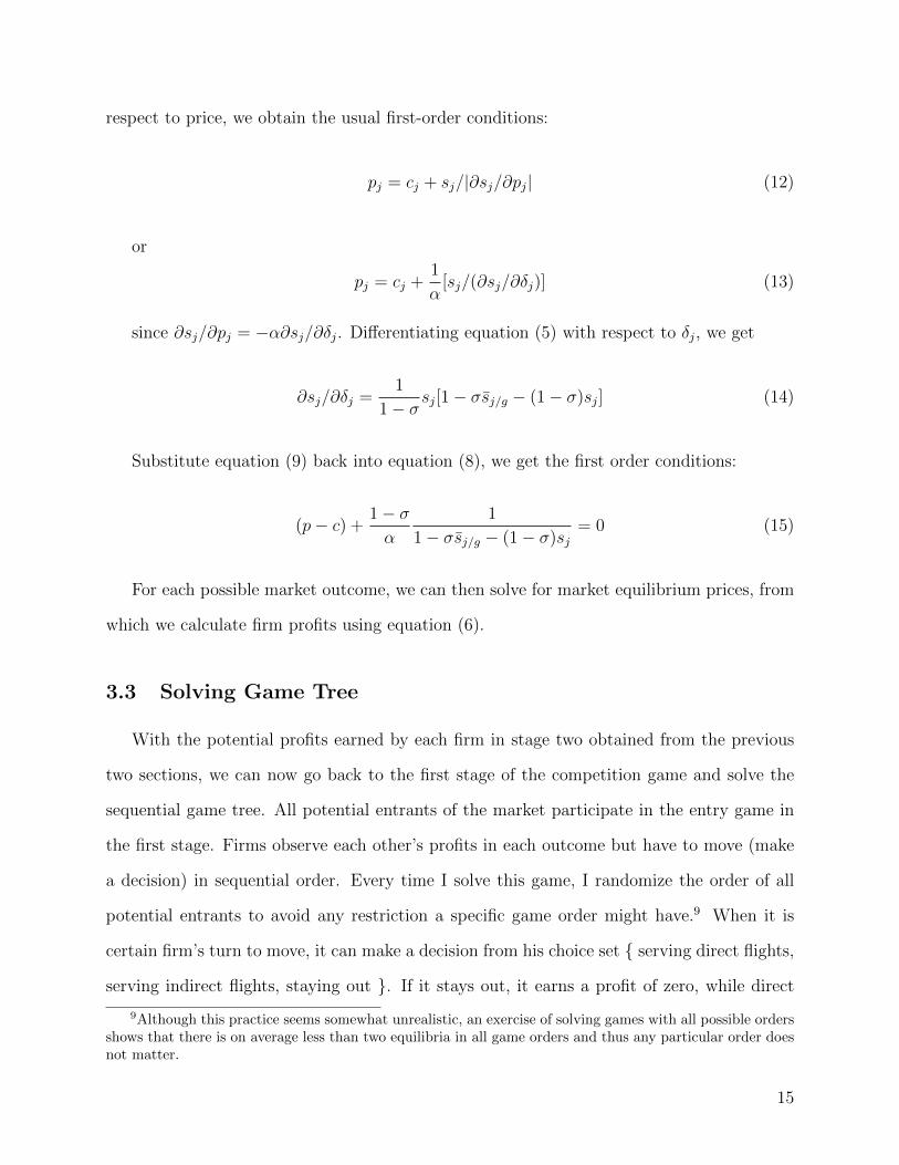
respect to price, we obtain the usual first-order conditions:

pj = cj + sj/|∂sj/∂pj| (12)

or

pj = cj +1

α[sj/(∂sj/∂δj)] (13)

since ∂sj/∂pj = −α∂sj/∂δj. Differentiating equation (5) with respect to δj, we get

∂sj/∂δj =1

1− σsj[1− σs̄j/g − (1− σ)sj] (14)

Substitute equation (9) back into equation (8), we get the first order conditions:

(p− c) +1− σα

1

1− σs̄j/g − (1− σ)sj= 0 (15)

For each possible market outcome, we can then solve for market equilibrium prices, from

which we calculate firm profits using equation (6).

3.3 Solving Game Tree

With the potential profits earned by each firm in stage two obtained from the previous

two sections, we can now go back to the first stage of the competition game and solve the

sequential game tree. All potential entrants of the market participate in the entry game in

the first stage. Firms observe each other’s profits in each outcome but have to move (make

a decision) in sequential order. Every time I solve this game, I randomize the order of all

potential entrants to avoid any restriction a specific game order might have.9 When it is

certain firm’s turn to move, it can make a decision from his choice set { serving direct flights,

serving indirect flights, staying out }. If it stays out, it earns a profit of zero, while direct

9Although this practice seems somewhat unrealistic, an exercise of solving games with all possible ordersshows that there is on average less than two equilibria in all game orders and thus any particular order doesnot matter.

15

and indirect flights’ profits were obtained from last two sections.

Now, in our example of three potential entrants, the game tree looks like the one in

Figure 5. With three firms, each with three choices, we have a total of 33 = 27 possible

outcomes, as shown in Figure 6, where 1 represents serving direct flights, 2 indirect flights,

and 0 represents staying out.

Figure 5: Game Tree

Figure 6: All Possible Outcomes

Accordingly, there is a profit matrix that has firms’ profits corresponding to each possible

outcome like Figure 7 (all numbers are made up for illustrative purposes).

Figure 7: Profit Matrix

To solve this game, we use backward induction on the profit matrix. First, let’s consider

firm C, who moves last. Given any possible combination of firm A and firm B’s decisions,

firm C would compare its profits associated with his three choices and make the decision

that would give it the highest profit. Thus, we can safely eliminate outcomes where C’s

profit is not optimal given A and B’s decisions, as shown in Figure 8. All outcomes that are

eliminated in the first round are shaded in black. Now similarly, for any decision of A, there

16

were nine possible outcomes, six of which were eliminated by C in the first round. Thus,

B is only left with three possible outcomes associated with its three choices. Therefore, the

game tree is effectively reduced to 2 layers (2 firms) and thus we could apply one more round

of elimination, as shown in Figure 9. Red blocks are the outcomes eliminated in the second

round. Now A is left with 3 choices and it would choose the one with the highest profit for

itself, as shown in Figure 10. Comparing the result with the original outcome matrix, we

know that the solution to this particular game is {A indirect, B direct, C direct}.

Figure 8: Profit Matrix after First Round of Eliminations

Figure 9: Profit Matrix after Second Round of Eliminations

Figure 10: Game Solution

4 Estimation

In order to estimate the model, I want to explain the variations in the data using our

model, and ultimately, how the observed and unobserved heterogeneity is explained by my

structural parameters. Thus, I make distributional assumptions about the unobserved char-

acteristics and estimate those distributions from which the key variables are drawn. In this

paper, I use the method of simulated moments (MSM) with an importance sampling esti-

mator proposed by Ackerberg (2009). Then I test the consistency of the estimator by Monte

17

Carlo simulations before I move to real world data, which is more noisy and unpredictable

in general.

4.1 Parameters

In the current version of the estimation, I assume that the parameters are distributed

as the following, where xjm is a vector of observed product characteristics of product j in

market m, and TRN(µ, σ2, a, b) is a truncated normal distribution with mean µ, standard

deviation σ, and truncated at a and b. LogN(µ, σ2) is a log normal distribution with mean

µ and standard deviation σ.

Direct Flight Quality: βjm ∼ N(xjmβ1, σ2

λ(Dm)), where β1 = β1,j+Dmβ2,τ(j)+Hubjmβ3,τ(j).

β1,j is the mean carrier-specific quality. Dm is the distance of market m, and λ(Dm) is a

binary variable that is equal to 1 if Dm > median(D) (long routes) and 0 otherwise. τ(j) is

also a binary variable that is equal to 1 if firm j (since each firm only produces one prod-

uct by assumption) is a Legacy carrier and 0 if it is a LCC carrier. This characterizes the

different effects of distance and hub on Legacy and LCC carriers.

Indirect service quality is specified as direct flight quality minus an indirect quality

penalty: βjm ∼ N(xjmβ2, σ2

p), where β2 = β4 +Dmβ5.

Price coefficient: αm ∼ LogN(βα, σ2α).

Nesting parameter (within-group correlation): σm ∼ TRN(βσ, σ2σ, 0.2, 0.95).

Marginal costs: Cjm ∼ TRN(xjmγ1, σ2

M , 0,∞), where γ1 = γ1,τ(j),φ(j) + Dmγ2,τ(j),φ(j) +

Hubγ3,τ(j),φ(j) and σM = σ1,τ(j),φ(j). φ(j) is a binary variable that is equal to 1 if product j

is providing direct service and 0 otherwise.

Fixed costs: Fjm ∼ TRN(xjmγ2, σ2

F , 0,∞), where γ2 = γ4,τ(j),φ(j) + Dmγ5,τ(j),φ(j) +

Hubγ6,τ(j),φ(j) and σF = σ2,τ(j),φ(j).

The set of structural parameters to be estimated is then

Γ = {β1, β2, β3, σλ(Dm), β4, β5, σp, βα, σα, βσ, σσ, γ1, γ2, γ3, σ1, γ4, γ5, γ6, σ2}.

And a draw of a set of parameters {βDirectjm , βIndirectjm , αm, σm, Cjm, Fjm} is called θt.

18

4.2 Importance Sampling Estimator

In this section, I will follow Ackerberg (2009) and Roberts and Sweeting (2011) to illus-

trate my estimation approach based on MSM with importance sampling. But the basic idea

is that I first generate a large number of simulations by solving my model described above

with some pre-specified set of structural parameters Γ0. Then I calculate moment functions

from both the simulations and data observations. Then when I search over the parameter

region of Γ for the optimal set of structural parameters, I re-weight my simulated moments

by likelihood functions of the realized draws θt and compare them with the data moments

to calculate my objective value (the value that I am minimizing throughout the estimation).

Formally, suppose we have n data observations. For each data observation, I take the

market-specific parameters from the data, i.e. market size, number of potential entrants,

number of LCC potential entrants, and market distance. Then together with a parameter

draw θt, I am able to solve my model described in the previous section. Repeat this process

and generate S simulations per data observation. All simulations are generated based on the

same pre-specified underlying structural parameters Γ0.

Let’s then define our moments as the following. Suppose we have k moments. For the

ith observation Wi in the data set, we define di,j(Wi) as the jth moment calculated from

that observation, e.g. AA market share given that AA has a hub.

In reality, I divide my moments into groups. In this version of the estimation, I first divide

the moments into 7 groups by the number of potential entrants in the market (ranging from

3 to 9). Then I further divide each of these groups into a group with short distance (less

than the median distance in the data sample), and one with long distance. Within each

group, we calculate 8 moments for each of the nine carriers (more on this later in the data

section), as shown in Table 1.

Thus I will end up with 14 groups with 72 moments in each group. Ultimately, moments

in each group are weighted by the number of observations (out of 1000 we sampled) in that

group when I construct the objective function.

19

Probability of AA entry as direct given hub statusProbability of AA entry as indirect given hub status

Average AA fare given hub statusAverage AA market share given hub status

Probability of AA entry as direct given non-hub statusProbability of AA entry as indirect given non-hub status

Average AA fare given non-hub statusAverage AA market share given non-hub status

Table 1: Sample Moments for AA

Let’s denote the simulation results obtained from a particular draw θj by yj, the likelihood

function is given by ∫fj(yj|θ)φ(θ|xj,Γ)dθ ≈ 1

S

S∑s=1

fj(yj|θs) (16)

where φ is the probability density function of the realized parameters given their respec-

tive distributions and the structural parameters used at that time. This would be the obvious

MSM estimator, but at the same time, it requires us to re-calculate fj and thus re-solve the

model every time the structural parameters change. Since we are searching for the optimal

set of parameters on many dimensions (we have quite a few parameters to estimate) and the

computation of fj is quite costly, the computational cost of this estimator is prohibitively

high.

What Ackerberg (2009) suggests is the following:

∫fj(yj|θ)φ(θ|xj,Γ)dθ =

∫fj(yj|θ)

φ(θ|xj,Γ)

g(θ|xj)g(θ|xj)dθ (17)

where g(θ|xj) is called the importance sampling density which does not depend on the

structural parameters Γ. Easily we can see that our estimator becomes

Es(Wi,Γ) =

∫fj(yj|θ)

φ(θ|xj,Γ)

g(θ|xj)g(θ|xj)dθ ≈

1

S

S∑s=1

fj(yj|θs)φ(θs|xj,Γ)

g(θs|xj)(18)

where θs is now a realized draw from the importance sampling density g. What this means

is that, since g does not depend on the structural parameters, we can calculate fj(yi|θs) once

20

and for all. During estimation, when the structural parameters change, all we have to do is

to re-compute φ(θs|xj,Γ) and re-weight our estimator in equation (13).

My moment function would then be

mn(Γ) = (mn,1(Γ), ...,mn,k(Γ))′ (19)

where mn,j(Γ) = n−1∑n

i=1(di,j(Wi)− Es(Wi,Γ)). I assume that

E[di,j(Wi)− Es(Wi,Γ∗)] = 0 (20)

where Γ∗ is the vector of true parameters. Thus, in practice, I search for Γ that mini-

mizes the norm of the moment vector mn(θ), with each moment weighted by the number of

observations in its moment group. Specifically, my objective function in the minimization

process is

F =k∑j=1

wj(mn,j(Γ))2 (21)

4.3 Monte Carlo Simulations

To test the consistency of this estimator before I am confident enough to move to data, I

ran several sets of Monte Carlo simulations. I first generate “data observations” by simulating

the above-mentioned games with parameters drawn from the specified a priori distributions

Γ0. In order to conduct the Monte Carlo simulations, I pretend that I know the “true

distribution” and let the importance sampling density g(θ|xj) = φ(θs|xj,Γ0). Then I estimate

the model exactly as described above to see whether I can recover the known true parameters.

Table 2 presents the Monte Carlo results from a previous model where I had one more

layer of nest and carriers only had two choices, i.e. entering and staying out.10 Although the

model is slightly different, I have developed the same estimator, and thus I show the results

10In the 3-level nested logit model, consumers first choose between flying versus other transportations.Conditional on flying, they choose between Legacy and LCC carriers. Within one category, they finallychoose which carrier to fly with.

21

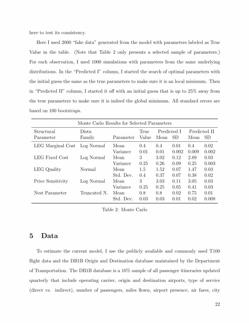
here to test its consistency.

Here I used 2000 “fake data” generated from the model with parameters labeled as True

Value in the table. (Note that Table 2 only presents a selected sample of parameters.)

For each observation, I used 1000 simulations with parameters from the same underlying

distributions. In the “Predicted I” column, I started the search of optimal parameters with

the initial guess the same as the true parameters to make sure it is an local minimum. Then

in “Predicted II” column, I started it off with an initial guess that is up to 25% away from

the true parameters to make sure it is indeed the global minimum. All standard errors are

based on 100 bootstraps.

Monte Carlo Results for Selected Parameters

Structural Distn True Predicted I Predicted IIParameter Family Parameter Value Mean SD Mean SD

LEG Marginal Cost Log Normal Mean 0.4 0.4 0.01 0.4 0.02Variance 0.01 0.01 0.002 0.009 0.002

LEG Fixed Cost Log Normal Mean 3 3.02 0.12 2.89 0.03Variance 0.25 0.26 0.09 0.25 0.003

LEG Quality Normal Mean 1.5 1.52 0.07 1.47 0.03Std. Dev. 0.4 0.37 0.07 0.38 0.02

Price Sensitivity Log Normal Mean 3 3.03 0.11 3.05 0.03Variance 0.25 0.25 0.05 0.41 0.03

Nest Parameter Truncated N. Mean 0.8 0.8 0.02 0.75 0.01Std. Dev. 0.03 0.03 0.01 0.02 0.008

Table 2: Monte Carlo

5 Data

To estimate the current model, I use the publicly available and commonly used T100

flight data and the DB1B Origin and Destination database maintained by the Department

of Transportation. The DB1B database is a 10% sample of all passenger itineraries updated

quarterly that include operating carrier, origin and destination airports, type of service

(direct vs. indirect), number of passengers, miles flown, airport presence, air fares, city

22

population, and etc. I use the T100 flight data to mainly identify airline hub status.

In cleaning up the data set, I only included domestic round trips with Economy class

tickets (fares ranging from $50 to $2000). A market is defined as a non-directional airport

pair. Some small carriers are aggregated into one carrier for computational costs consider-

ations: AA, CO, DL, NW, UA, US, other Legacy, WN, other LCC. I also want to exclude

services that served less than 15 sampled passengers (150 in actuality) during a quarter.

A potential entrant is then defined as a carrier who serves both endpoints of a particular

market. Since I assume that each carrier only produces one product in a particular market,

I choose the service of the carrier that has the most passengers.

For the current estimation, I restrict the data set to Q2 of 2008 to focus on the effects

of Delta-Northwest merger. I then sampled the data set to 1000 airport-pair markets based

on market sizes. The sampled relevant markets are relatively large markets, with endpoint

cities having more than 500,000 population. Table 3 below shows some summary statistics

for key variables of interests.

Summary Statistics of the Current Sample

Variable # of Obs. Mean SD 10th Percentile 90th Percentile

Potential Entrant 1000 7.6 1.1 6 9Legacy PE 1000 6.3 0.9 5 7LCC PE 1000 1.3 0.6 1 2Entrants 1000 4.0 1.7 2 6Direct Entrants 1000 0.9 1.0 0 2Indirect Entrants 1000 3.0 1.6 1 5Hub Status 9000 0.19 0.15 0 1Hub if direct 938 0.63 0.23 0 1Fare 3978 390.21 92.53 283.98 510.65Direct Fare 938 403.56 113.61 277.96 564.84Indirect Fare 3040 386.09 84.58 285.64 497.63Market Share 3978 0.060 0.089 0.008 0.155Direct Share 938 0.156 0.138 0.016 0.359Indirect Share 3040 0.030 0.026 0.008 0.064

Table 3: Summary Statistics

23

6 Results

For the current estimation, I used 250 simulations for each of the 1000 sampled markets

and obtained the estimates for the structural parameters that describe the perceived qualities

of product characteristics (demand side) as shown in Table 4. All standard errors are based

on a random bootstrap of 100 repetitions. Table 5 presents other demand-side parameters

including the price sensitivity coefficient α, nesting parameter σ that quantifies within-group

correlation, and the indirect penalty which describes the difference between the perceived

qualities of the same product (for both Legacy and LCC carriers) serving direct and indirect.

In Table 6, we show estimates of marginal and fixed costs parameters for different types of

services.

With these estimates, Table 7 presents a selected sample (to be consistent with the

example above) of all the moments associated with AA in the group (out of the 14 moment

groups) where there are 7 potential entrants and above-median distance. There are 139

observations out of the total 1000 observations that fall in this group, and thus the difference

between the moments of simulations and data moments is weighted by 0.139 in the objective

function in the optimization process.

Among these estimates, hub dominance (Table 4) gives carriers a big boost in their

perceived quality among consumers. Price sensitivity (Table 5) is fairly sensible and increases

in both magnitude and variance with distance. Penalty in perceived quality of product

decreases with distance, which reflects the fact that people are more willing to take indirect

flights when the travel distance is long. On the supply side (Table 6), hub status always

reduces fixed costs, but increases marginal costs for LCC carriers and indirect marginal costs

for Legacy carriers. This is probably the result of the strategic entry and selection of hubs

of LCC carriers. Once we introduce some exogenous cost shifters into the model in future

research, this might turn out differently. All marginal costs go up with longer distance, while

24

most fixed costs go down with longer distance.

Qualities

Legacy Carriers LCC CarriersMean Std. Dev. Mean Std. Dev.

AA 0.6579 (0.0453) WN 1.5553 (0.1031)CO -0.0436 (0.0499) Other LCC 0.4522 (0.0698)DL 0.7842 (0.0431) Distance -0.0864 (0.0326)NW 0.3447 (0.0444) Hub -0.0908 (0.1240)UA 0.8104 (0.0468) Short Std. 0.7815 (0.0318)US 0.4408 (0.0457) Long Std. 0.6526 (0.0485)Other LEG -0.1747 (0.0666)Distance 0.0127 (0.0177)Hub 0.9355 (0.0435)Short Std. 0.6945 (0.0129)Long Std. 0.8015 (0.0199)

Table 4: Estimates of Quality Parameters

Other Demand Parameters

Price Sensitivity α Nesting Parameter σ Indirect PenaltyMean Std. Dev. Mean Std. Dev. Mean Std. Dev.

Constant 0.3029 (0.0100) Mean 0.5339 (0.0072) Constant 1.0153 (0.0190)Distance 0.0879 (0.0055) Std. 0.1343 (0.0068) Distance -0.1653 (0.0084)Short Var. 0.0062 (0.0008) Std. 0.3132 (0.0047)Long Var. 0.0255 (0.0030)

Table 5: Estimates of Other Demand Parameters

25

Cost Parameters

Marginal Costs, Direct

Legacy Carriers LCC CarriersMean Std. Dev. Mean Std. Dev.

Constant 2.0966 (0.0508) Constant 1.1289 (0.1109)Distance 0.5566 (0.0246) Distance 0.4708 (0.0428)Hub -0.2506 (0.0664) Hub 0.3934 (0.1029)Std. 0.9705 (0.0155) Std. 0.7212 (0.0247)

Marginal Costs, Indirect

Legacy Carriers LCC CarriersMean Std. Dev. Mean Std. Dev.

Constant 1.2205 (0.0403) Constant 1.7031 (0.1374)Distance 0.7669 (0.0180) Distance 0.6847 (0.0505)Hub 0.2004 (0.0458) Hub 0.2162 (0.1553)Std. 0.7963 (0.0170) Std. 1.1068 (0.0448)

Fixed Costs, Direct

Legacy Carriers LCC CarriersMean Std. Dev. Mean Std. Dev.

Constant 3.7276 (0.0378) Constant 4.5748 (0.0932)Distance 0.1223 (0.0158) Distance -0.1836 (0.0394)Hub -0.1168 (0.0394) Hub -0.477 (0.1125)Std. 0.4848 (0.0210) Std. 0.6946 (0.0600)

Fixed Costs, Indirect

Legacy Carriers LCC CarriersMean Std. Dev. Mean Std. Dev.

Constant 0.6718 (0.0220) Constant 0.4815 (0.0367)Distance -0.0714 (0.0063) Distance -0.0501 (0.0094)Std. 0.525 (0.0543) Std. 0.2362 (0.0626)

Table 6: Estimates of Quality Parameters

26

Sample Moments Fit

7 Potential Entrants, Long RoutesMoments # of Obs. Data Predicted

AA entry direct hub 139 0.0288 0.0143AA entry indirect hub 139 0.1655 0.1659AA price hub 139 0.8994 0.9468AA share hub 139 0.0095 0.0222AA entry direct non-hub 139 0.0072 0.0027AA entry indirect non-hub 139 0.5324 0.4121AA price non-hub 139 2.1722 2.1692AA share non-hub 139 0.0230 0.0421

Table 7: Sample Moments Fit

7 Counterfactuals

With the current estimated model, I will investigate the merger endogeneity much in

a similar fashion as the Cournot model at the beginning of the paper by conducting the

following counterfactuals.

Consider the route from Atlanta to Detroit (ATL-DTW market) in 2008 Q2. In this

market, as shown in Table 8, there are 5 incumbents and 2 potential entrants. All 7 carriers

participate in the entry game, in which we define a natural order: DL, NW, FL, US, UA,

AA, CO, based on their hub status, type of service, and market share (again, I can make this

assumption because the game order only matters to some extent - there are on average less

than 2 equilibria among all possible orders). Given the five incumbents’ observed prices and

market shares, I can solve for their implied qualities and marginal costs associated with their

type of service (e.g. I can only solve for direct qualities for DL because DL is flying direct

on that route) by minimizing the difference between model-predicted and observed prices

and market shares. I then draw the rest of the parameters from the estimated distributions.

For now, I keep α and σ at their respective mean (so it is easier to collect useful games

in the following steps). Then I first simulate 5000 games with the implied parameters and

parameters drawn from estimated distributions. Out of the 5000 simulated games, I collected

1853 games that matched the actual outcome of the entry game, i.e. Northwest entered as

27

direct, Delta entered as direct, AirTran entered as direct, United entered as indirect, US

Airways entered as indirect, and American and Continental did not enter.

ATL-DTW Market in 2008 Q2

Carrier Hub Service Fare Passengers

Delta (DL) Y Direct 334.42 15960Northwest (NW) Y Direct 315.77 19210AirTran (FL) Y Direct 263.49 9870US Airways (US) N Indirect 399.41 330United (UA) N Indirect 230.44 160American (AA) N Potential - -Continental (CO) N Potential - -

Table 8: Market Summary I

I consider these 1853 games as my base set (call it set A) of market simulations, out

of which I can simulate mergers. To simulate a merger between Northwest and Delta, I

take out Northwest, give Delta the mean marginal costs, qualities (both direct and indirect)

of the two. Keeping everything else the same (same move orders and parameter draws), I

re-simulate these 1853 games and store the results in set B. Then I simulate two mergers

between FL and US: one conditional on set A and store the results in set C, the other

conditional on set B and store in set D.

Similar to the motivating example in the introduction, I am interested in the incentive

for firms to merge, which is measured in the profitability of the merger, i.e. the change of

profits of the merging firms before and after the merger. Specifically, let

π1 = π(FL|DL, NW, FL, US, others) + π(US|DL, NW, FL, US, others) (22)

π2 = π(FL-US|DL, NW, FL-US, others) (23)

π3 = π(FL|DL-NW, FL, US, others) + π(US|DL-NW, FL, US, others) (24)

π4 = π(FL-US|DL-NW, FL-US, others) (25)

I = (π4 − π3)− (π2 − π1) (26)

(π2 − π1) is the incentive for AirTran and US Airways to merge in the current market.

28

(π4−π3) is the incentive for them to merge given that Delta and Northwest completed their

merger in the market. Therefore, I is the extra incentive for AirTran and US Airways to

merge provided by the DL-NW merger.

Counterfactual Results: ATL-DTW

Min Max Mean % Positive

π1 5.34 14.12 11.57 100%π2 5.33 31.78 12.88 100%π3 22.97 31.74 29.17 100%π4 23.41 54.10 31.48 100%(π2 − π1) -0.22 19.17 1.31 57%(π4 − π3) -5.50 27.00 2.31 89%I -5.55 8.38 1.00 98%

Table 9: Counterfactual Results I

Table 9 presents the counterfactual results, in which the last column means what per-

centage of the 1853 game results are positive. Out of 1853 games, only 57% of the FL-US

mergers are profitable initially. After DL and NW merged, however, 89% of the FL-US

mergers would be profitable. About 33% of the FL-US mergers changed from non-profitable

to profitable after the DL-NW merger, while only 0.7% of the FL-US mergers changed from

profitable to non-profitable. Overall, 98% of the extra incentive to merge for FL and US

from the DL-NW merger are positive and thus, the DL-NW merger would at least to some

extent increase the probability of a merger between FL and US.

I then perform the same counterfactual analysis on a different market with more relevant

carriers in terms of current industry focus. Table 10 presents a market summary of the

ABQ-CLT market just like Table 8. In simulating the market to match the market outcome

this time, however, I was only able to collect 526 games out of 20,000 simulations. Then

out of these 526 games, I again simulate a first merger between Delta and Northwest and

a second merger between American and US Airways, and study how the DL-NW merger

affects the potential AA-US merger, which is more in line with what is happening in the

news. Table 11 shows the results I get with this counterfactual. Initially, only 21% of the

29

US-AA mergers are profitable, while after the DL-NW merger, there are 40% of them that

are profitable. 19.2% of the US-AA mergers changed from non-profitable to profitable after

the DL-NW merger, while only 1 out of 526 (0.2%) changed in the other direction. Finally,

89% of the extra incentive for US and AA to merge from the DL-NW merger are positive,

suggesting the positive correlation between mergers.

ABQ-CLT Market in 2008 Q2

Carrier Hub Service Fare Passengers

US Airways (US) Y Indirect 459.49 390Northwest (NW) Y Indirect 328.89 160American (AA) N Indirect 429.12 790Dleta (DL) N Indirect 469.08 520Continental (CO) N Potential - -United (UA) N Potential - -

Table 10: Market Summary II

Counterfactual Results: ABQ-CLT

Min Max Mean % Positive

π1 0.25 1.28 0.90 100%π2 0.20 0.99 0.77 100%π3 0.05 1.49 1.10 100%π4 0.34 1.30 1.06 100%(π2 − π1) -0.71 0.53 -0.13 21%(π4 − π3) -0.77 0.72 -0.04 40%I -0.41 0.58 0.09 89%

Table 11: Counterfactual Results II

8 Conclusions

In this paper, I constructed and estimated a preliminary structural model of the U.S.

airline industry that takes into account the entry selection bias based on firms’ costs and

qualities. In estimating demand, I incorporated a standard discrete-choice nested logit model

for differentiated products market. The structural model is estimated with the method of

30

simulated moments and an importance sampling estimator. Finally, I drew my conclusion

upon this model by conducting counterfactual analysis of merger simulations and revealing

some empirical evidence of positive correlation between consecutive mergers.

Specifically, from a firm’s perspective, I found that a potential merger’s profitability in

a given market is usually substantially augmented by a previous merger. In spirit of recent

news, what I found means that, given Delta and Northwest has completed their merger in

many markets (airport-to-airport routes), there is now a much higher incentive for other

carriers in the same markets to merge, e.g. United and Continental, and American and US

Airways, which to some extent explains the recent series of airline mergers.

This paper contributes to the current existing literature in the following ways. Merger

analysis has long been done in a static model based on the assumption that mergers are

exogenous. Studies of dynamic models in differentiated product markets like the U.S. air-

line market have been extremely limited to only theoretical analysis. This paper presents

empirical results from repeatedly solving a static model, suggesting the endogenous nature

of airline mergers. Another interesting aspect of this paper is that it is based on a selective

entry model, where the selection bias of entry is addressed and adjusted, which would in

turn affect the post-entry competition in the market.

This paper also has important implications to the antitrust authorities. Traditional

myopic antitrust policies only focus on the simulated welfare effects of the current merger

under review. Nocke and Whinston (2010) suggests that, in a Cournot setting, myopic

antitrust policies work as well as any forward-looking policies. However, in a differentiated

product market with Bertrand competition, strong assumptions about firms’ costs have to be

made in order to reach the same conclusion. Thus, our exercise based on the selective entry

model is in place to suggest that in a forward-looking antitrust policy, antitrust authorities

have to be more cautious about approving airline mergers due to the entry selection bias

and the potential domino effect induced by the current merger.

Going forward from the current paper, there are several directions that I would like to

31

further explore. First and foremost, I am eager to attempt to develop a fully functional

dynamic model of the U.S. airline industry that takes into account the dynamic interplay

of merger, investment, entry and exit much similar to Gowrisankaran (1999). Second, the

current model is fully capable of more advanced identification methods such as generalized

method of moments proposed by Andrews and Soares (2010), by which I might obtain more

accurate estimates. Third, several new model specifications will be introduced such as carrier

aggregation, cost shifters, and etc. Fourth, a model will be estimated with a data set up to

2011 Q3 to investigate effects of Delta-Northwest merger, United-Continental merger, and

potential effects of American-US Airways merger.

References

Ackerberg, D. (2009) “A new use of importance sampling to reduce computational burdenin simulation estimation,” Quant Mark Econ, 7, 343-376.

Armantier, O. and O. Richard (2008) “Domestic Airline Alliances and Sonsumer Welfare,”The RAND Journal of Economics, 39, 875-904.

Bailey, E. and A. Friedlaender (1982) “Market Structure and Multiproduct Industries,”Journal of Economic Literature, 20, 1024-1048.

Bailey, E. and J. Panzar (1981) “The Contestability of Airline Markets during the Transitionto Deregulation,” Law and Contemporary Problems, 44, 125-146.

Bailey, E. and W. Baumol (1983) “Deregulation and the theory of contestable markets,” TheYale Journal on Regulation, 1, 111-138.

Baker, J. and T. Bresnahan (1985) “the Gains from Merger or Collusion in Product-Differentiated Industries,” Journal of Industrial Economics, 33, 427-444.

Berry, S. (1992) “Estimation of a Model of Entry in the Airline Industry,” Econometrica,60, 889-917.

Berry, S. (1994) “Estimating Discrete-Choice Models of Product Differentiation,” The RANDJournal of Economics, 25, 242-262.

Berry, S. and A. Pakes (1993) “Some Applications and Limitations of Recent Advances inEmpirical Industrial Organization Merger Analysis,” The American Economic Review, 83,247-252.

Berry, S., M. Carnall, and P. Spiller (2006) “Airline Hubs: Costs, Markups, and the Implica-tions of Customer Heterogeneity,” Advances in Airline Economics: Competition Policy andAntitrust, 1, ed. Darin Lee, 183-214. Amsterdam: Elsevier.

32

Berry, S., J. Levinsohn, and A. Pakes (1995) “Automobile Prices in Market Equilibrium,”Econometrica, 63, 841-890.

Borenstein, S. (1989) “Hubs and High Fares: Dominance and Market Power in the U.S.Airline Industry,” RAND Journal of Economics, 20, 344-365.

Borenstein, S. (1990) “Airline Mergers, Airport Dominance, and Market Power,” AmericanEconomic Review Papers and Proceedings, 80.

Borenstein, S. (1992) “The Evolution of US Airline Competition,” Journal of EconomicPerspectives, 6, 45-73.

Brueckner, J., N. Dyer, and P. Spiller (1992) “Fare Determination in Airline Hub-and-SpokeNetworks,” RAND Journal of Economics, 23, 309-333.

Brueckner, J. and P. Spiller (1991) “Competition and Mergers in Airline Networks,” Inter-national Journal of Industrial Organization, 106, 323-342.

Cheong, K.-S. and K. Judd (1992) “Mergers and Dynamic Oligopoly,” Mimeo, Hoover In-stitution, Stanford University.

Ciliberto, F., and E. Tamer (2009) “Market Structure and Multiple Equilibria in AirlineMarkets,” Econometrica, 77, 1791-1828.

Dube, J.-P. (2005) “Product Differentiation and Mergers in the Carbonated Soft DrinkIndustry,” Journal of Economics & Management Strategy, 14, 879-904.

Ericson, R. and A. Pakes (1995) “Markov-Perfect Industry Dynamics: A Framework forEmpirical Work,” Review of Economic Studies, 62, 53-82.

Gowrisankaran, G. (1999) “A Dynamic Model of Endogenous Horizontal Mergers,” TheRAND Journal of Economics, 30, 56-83.

Hausman, J. G. Leonard, and D. Zona (1994) “Competitive Analysis with DifferentiatedProducts,” Annales d’Economie et de Statistique, 0, 159-180.

Ito, H. and D. Lee (2006) “Market Density and Low Cost Carrier Entries in the U.S. AirlineIndustry: Implications for Future Growth,” Low Cost Carriers: A Global Experience, IBSPress, 2006.

Kim, E. and V. Singal (1993) “Mergers and Market Power: Evidence from the AirlineIndustry,” American Economic Review, 83, 549-569.

Levine, M. (1987) “Airline Competition in Deregulated Markets: Theory, Firm Strategy,and Public Policy,” Yale Journal on Regulation, 4, 393-494.

Morrison, S. and C. Winston (1987) “Empirical Implications and Tests of the ContestabilityHypothesis,” Journal of Law and Economics, 30, 53-66.

33

Nevo, A. (2000) “Mergers with Defferentiated Products: The Case of the Ready-to-EatCereal Industry,” The RAND Journal of Economics, 31, 395-421.

Nocke, V. and M. Whinston (2010) “Dynamic Merger Review,” The Journal of PoliticalEconomy, 118, 1201-1251.

Peters, C. (2006) “Evaluating the Performance of Merger Simulation: Evidence from theU.S. Airline Industry,” Journal of Law and Economics, 49, 627-649.

Reiss, P. and P. Spiller (1989) “Competition and Entry in Small Airline Markets,” Journalof Law and Economics, vol. XXXII.

Roberts, J. and A. Sweeting (2011): “Competition versus Auction Design,” NBER WorkingPaper 16650.

Roberts, J. and A. Sweeting (2011): “Airline Mergers and the Potential Entry Defense,”Working Paper, Duke University.

Werden, G. and L. Froeb (1994) “The Effects of Mergers in Differentiated Products Indus-tries: Logit Demand and Merger Policy,” Journal of Law, Economics, and Organization, 10,407-426.

34