VA-502-06-TR SERDP SEED PROJECT UX-1451 FINAL REPORT

EMPIRICAL CORRECTIONS TO DIPOLE MODEL

October 2006 PERFORMING ORGANIZATION AETC Incorporated 1225 South Clark Street, Suite 800 Arlington, VA 22202 PRINCIPAL INVESTIGATOR Jonathan Miller This research was supported wholly by the U.S. Department of Defense, through the Strategic Environmental Research and Development Program (SERDP) through Project UX-1451 under Contract W912HQ-05-P-0034.

VIEWS, OPINIONS, AND/OR FINDINGS CONTAINED IN THIS REPORT ARE THOSE OF THE AUTHOR(S) AND

SHOULD NOT BE CONSTRUED AS AN OFFICIAL DEPARTMENT OF THE ARMY POSITION, POLICY, OR

DECISION, UNLESS SO DESIGNATED BY OTHER OFFICIAL DOCUMENTATION.

Distribution Statement A: Approved for Public Release, Distribution is Unlimited

Report Documentation Page Form ApprovedOMB No. 0704-0188

Public reporting burden for the collection of information is estimated to average 1 hour per response, including the time for reviewing instructions, searching existing data sources, gathering andmaintaining the data needed, and completing and reviewing the collection of information. Send comments regarding this burden estimate or any other aspect of this collection of information,including suggestions for reducing this burden, to Washington Headquarters Services, Directorate for Information Operations and Reports, 1215 Jefferson Davis Highway, Suite 1204, ArlingtonVA 22202-4302. Respondents should be aware that notwithstanding any other provision of law, no person shall be subject to a penalty for failing to comply with a collection of information if itdoes not display a currently valid OMB control number.

1. REPORT DATE OCT 2006

2. REPORT TYPE Final

3. DATES COVERED -

4. TITLE AND SUBTITLE Empirical Corrections to Dipole Model

5a. CONTRACT NUMBER

5b. GRANT NUMBER

5c. PROGRAM ELEMENT NUMBER

6. AUTHOR(S) Jonathan Miller

5d. PROJECT NUMBER MM-1451

5e. TASK NUMBER

5f. WORK UNIT NUMBER

7. PERFORMING ORGANIZATION NAME(S) AND ADDRESS(ES) SAIC (formerly AETC Inc.) 1225 South Clark Street, Suite 800Arlington, VA 22202

8. PERFORMING ORGANIZATIONREPORT NUMBER VA-502-06-TR

9. SPONSORING/MONITORING AGENCY NAME(S) AND ADDRESS(ES) Strategic Environmental Research & Development Program 901 N StuartStreet, Suite 303 Arlington, VA 22203

10. SPONSOR/MONITOR’S ACRONYM(S) SERDP

11. SPONSOR/MONITOR’S REPORT NUMBER(S)

12. DISTRIBUTION/AVAILABILITY STATEMENT Approved for public release, distribution unlimited

13. SUPPLEMENTARY NOTES The original document contains color images.

14. ABSTRACT

15. SUBJECT TERMS

16. SECURITY CLASSIFICATION OF: 17. LIMITATION OF ABSTRACT

UU

18. NUMBEROF PAGES

22

19a. NAME OFRESPONSIBLE PERSON

a. REPORT unclassified

b. ABSTRACT unclassified

c. THIS PAGE unclassified

Standard Form 298 (Rev. 8-98) Prescribed by ANSI Std Z39-18

This report was prepared under contract to the Department of Defense Strategic Environmental Research and Development Program (SERDP). The publication of this report does not indicate endorsement by the Department of Defense, nor should the contents be construed as reflecting the official policy or position of the Department of Defense. Reference herein to any specific commercial product, process, or service by trade name, trademark, manufacturer, or otherwise, does not necessarily constitute or imply its endorsement, recommendation, or favoring by the Department of Defense.

Table of Contents List of Figures ................................................................................................................................. 3 Acknowledgments........................................................................................................................... 4 Acronyms........................................................................................................................................ 4 Executive Summary ........................................................................................................................ 5 1. Project Objective......................................................................................................................... 6 2. Background................................................................................................................................. 6 2.1 The Dipole Model ............................................................................................................... 6 2.2 Advantages of the Dipole Model ........................................................................................ 7 2.3 Disadvantages of the Dipole Model.................................................................................... 7 2.4 Correcting the Dipole Model .............................................................................................. 8 3. Methods..................................................................................................................................... 12 3.1 The Look-up Table ........................................................................................................... 12 3.2 Populating the Look-up Table .......................................................................................... 13 3.3 The BOR.exe target .......................................................................................................... 14 4. Accomplishments...................................................................................................................... 14 4.1 ERDC Test Stand Measurements...................................................................................... 14 4.2 Background Signals at ERDC........................................................................................... 15 5. Results and Discussion ............................................................................................................. 17 5.1 Method of evaluation ........................................................................................................ 17 5.2 Evaluation with the ERDC dataset ................................................................................... 17 5.3 Evaluation with the BOR.exe dataset ............................................................................... 17 6. References................................................................................................................................. 21

2

List of Figures Figure 1. A small steel cylinder was moved through five positions along the x axis ................... 7 Figure 2 The 4-inch steel cylinder was positioned on a lattice ..................................................... 9 Figure 3 The Dipole Model fit to data (top set) shows discrepancies.. ....................................... 10 Figure 4 This contour plot shows the spatial distribution of the empirical correction factors. ... 11 Figure 5 Sensor – target geometry is defined using three angles and one length. ....................... 12 Figure 6. A graph of ranked correction values for all 6655 nodes in the lattice. ........................ 12 Figure 7. Contour graphs showing a 2-dimensional cut through the look-up table..................... 13 Figure 8. The ellipsoid target used in the BOR.exe code. ........................................................... 14 Figure 9. The 81mm mortar round measured on the ERDC test stand........................................ 14 Figure 10. The GEM3 sensor was attached to a carriage on the gantry. ..................................... 14 Figure 11. The sampling locations for the GEM3.. ..................................................................... 15 Figure 12. Background signals measured with at various locations............................................ 16 Figure 13. Processed GEM3 data for the sphere in the calibration area...................................... 16 Figure 14. Beta estimates from the ERDC dataset. ..................................................................... 18 Figure 15. Standard Dipole Model results and results using the look-up table corrections. ....... 19 Figure 16. The beta values used to generate Dipole Model predictions...................................... 20

3

Acknowledgments This project was funded fully by SERDP under project UX-1451 through contract W912HQ-05-P-0034.

Acronyms BOR Body of Revolution EMI Electromagnetic Induction. ERDC Engineer Research and Development Center GEM3 Sensor model manufactured by Geophex. GUI Graphical User Interface. IDL Interactive Data Language. A programming language. JPG Jefferson Proving Ground, IN. Rx Receiver SERDP Strategic Environmental Research and Development Program. Tx Transmitter UXO Unexploded Ordnance WES Waterways Experiment Station

4

Executive Summary We successfully demonstrated an empirical approach for correcting errors in the standard Dipole Model of EMI response. The Dipole Model [1,2] is accurate for small targets at relatively deep burial depths but it breaks down for larger targets at shallower depths because of the interaction between the target body and the spatially non-uniform primary field. Our approach was to calculate this interaction numerically for a large set of specific target-sensor geometries using the BOR.exe code developed in 2004 by Fridon Shubitidze and Irma Shamatava for a SERDP project, and then find empirical correction factors which adjust Dipole Model predictions to match the calculated results. The correction factors were assembled into a large look-up table, from which arbitrary target-sensor geometries can be queried through multi-linear interpolation. This approach is sensor-specific and target specific, but the results will indicate the seriousness of the corrections required, and it was originally thought that the results are likely to carry over to other geometries and scales. We incorporated the look-up table into a code that recovers target response parameters (beta values) from position-referenced sensor signals, and demonstrated application on a synthetic dataset generated by BOR.exe and a GEM3 dataset collected at the ERDC test stand in Vicksburg MS. To evaluate the usefulness of the empirical correction, repeated trials were performed in which random sub-samples of position-referenced EMI data were drawn and inverted twice: once using the standard Dipole Model, and a second time using the standard Dipole Model with the new empirical correction. The observed spread in results over many trials provided an estimate of uncertainty. Results show that the empirical correction produce marked improvement in consistency when applied to the synthetic dataset but not for the ERDC dataset. We speculate this could be because the ERDC data may be corrupted due to a malfunctioning GEM3 sensor, or possibly because the ERDC target was an 81mm mortar round, and our correction look-up table was based on numerical results for a homogeneous ellipsoid. This latter possibility suggests that Dipole Model corrections might not carry over across similar geometries and scales as well as hoped. This leaves open the possibility that more detailed numerical computations could be used to reduce Dipole Model errors on heterogeneous targets like mortars; however the computational tradeoff would have to be considered.

5

1. Project Objective The objective was to demonstrate improved discrimination of one UXO type (81mm mortar) using one EMI sensor (Geophex GEM3), by developing a straightforward, purely empirical correction to the Dipole Model. In the process, we also evaluated the magnitude of error in the Dipole Model, and developed a modified version of BOR.exe which translates inputs and outputs to our IDL coding environment, and allows complicated processing jobs to be batch-processed. 2. Background 2.1 The Dipole Model Analysis of EMI data can be approached as an inversion problem in which models that relate target attributes to associated EMI response are required. Such models can be derived analytically for only a few targets, e.g., a sphere [3], a cylinder of infinite length oriented transverse to the primary field [4], and multiple conducting loops [3]. While numerical models provide useful results for a variety of additional target types, e.g., bodies of revolution [2], and targets of arbitrary shape [5], they are not suitable for data inversion due to long computation times. The Dipole Model is a widely used method of predicting response based on the geometry of the target and sensor. In the Dipole Model, response is represented as an induced dipole moment m located at a single point in space (typically considered the center of the buried target), which is linearly related to the primary field H at that point, through the magnetic polarizability tensor B; m = B · H. (1) B can be diagonalized with a suitable rotation matrix U, which aligns the coordinate system with the target’s principal axes;

. (2) TUβ

ββ

U⎥⎥⎥

⎦

⎤

⎢⎢⎢

⎣

⎡=

3

2

1

000000

B

The β1, β2, β3, or “beta values” are eigenvalues of B and represent response along the three principal axes of the target. They are frequency-dependent, and comprise the information on which many target discrimination schemes are based.

6

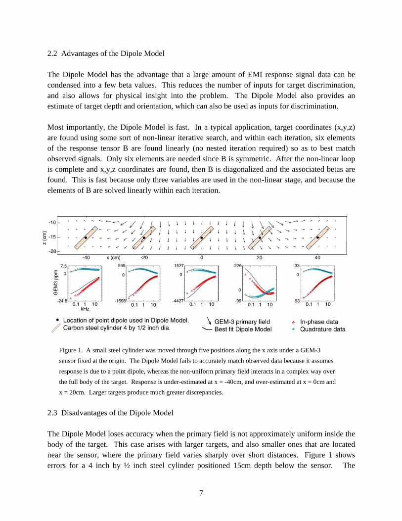
2.2 Advantages of the Dipole Model The Dipole Model has the advantage that a large amount of EMI response signal data can be condensed into a few beta values. This reduces the number of inputs for target discrimination, and also allows for physical insight into the problem. The Dipole Model also provides an estimate of target depth and orientation, which can also be used as inputs for discrimination. Most importantly, the Dipole Model is fast. In a typical application, target coordinates (x,y,z) are found using some sort of non-linear iterative search, and within each iteration, six elements of the response tensor B are found linearly (no nested iteration required) so as to best match observed signals. Only six elements are needed since B is symmetric. After the non-linear loop is complete and x,y,z coordinates are found, then B is diagonalized and the associated betas are found. This is fast because only three variables are used in the non-linear stage, and because the elements of B are solved linearly within each iteration.

Figure 1. A small steel cylinder was moved through five positions along the x axis under a GEM-3 sensor fixed at the origin. The Dipole Model fails to accurately match observed data because it assumes response is due to a point dipole, whereas the non-uniform primary field interacts in a complex way over the full body of the target. Response is under-estimated at x = -40cm, and over-estimated at x = 0cm and x = 20cm. Larger targets produce much greater discrepancies.

2.3 Disadvantages of the Dipole Model The Dipole Model loses accuracy when the primary field is not approximately uniform inside the body of the target. This case arises with larger targets, and also smaller ones that are located near the sensor, where the primary field varies sharply over short distances. Figure 1 shows errors for a 4 inch by ½ inch steel cylinder positioned 15cm depth below the sensor. The

7

inaccuracy arises from the fact that conducting targets of arbitrary shape and arbitrary permeability produce complex response in the presence of spatially non-uniform primary fields. Note the inverted response in the second graph from the right in figure 1. This results from the fact that the transmit coil and receive coil on the GEM3 do not have the same radius, and therefore the transmit (Tx) and receive (Rx) fields do not always point in the same direction. When a long slender object like this rod is positioned such that axial component of the Tx field points opposite to the axial component of the Rx field, then the signal inverts because the normal eddy currents excited in the target produce the opposite effect in the Rx coil. (Here, “axial component” refers to the projection of the given field onto the principal axis of the target.) This effect only occurs with long slender objects at certain angles. Note that the Dipole Model succeeds in predicting this effect, although there is some error in magnitude. The Dipole Model also produces errors in depth estimates, depending on target orientation. In general, a sharp local “spike” (spatially) in EMI response indicates a shallow target, whereas a wide, low “bump” indicates a deep target. This leads to a bias in depth predictions from the Dipole Model when applied to long, slender objects like typical UXO. When the target is vertical, EMI response directly overhead is exaggerated, because the near part of the target is excited more strongly than expected under the point-target assumption. This makes the EMI field appear to be more “spiked”, leading to under-prediction of target depth. On the other hand, when the target is horizontal, the ends of the target couple more strongly with the diverging fields of the sensor when it is located off-center, tending to make the EMI field appear broader than it would be under the point-target assumption, leading to over-prediction of target depth. The Dipole Model also results in distorted estimates of beta response values when used as an inversion tool. Since beta values are widely used as inputs for target discrimination and identification algorithms, this distortion can be important. 2.4 Correcting the Dipole Model Figures 2, 3, and 4 illustrate empirical correction factors to the Dipole Model based on GEM3 data. Corrections were found using least-squares minimization on each measurement point to find the linear combination of β values that best represents observed data. The corrections are expressed as coefficients on the β values, depending on the target orientation and position relative to the sensor. The contoured data in figure 4 shows correction factors for the transverse response (β value), and it appears to be a smoothly varying function of target x, y position, leading to the idea that correction factors may generally be found by interpolating between a fixed set of values determined empirically. The goal of this project is to determine many more contour surfaces similar to those in figure 4, to extend their dimensions so they include

8

dependence on target azimuth and target elevation, and to represent them in a multi-dimensional table. They may then be rapidly queried and used to accurately re-create the spatial dependence of UXO response for comparison with field data.

Figure 2 The 4-inch steel cylinder was positioned on a lattice of 25 measurement points and fitted to a Dipole Model using axial beta values determined from separate test stand measurements along the principal axes. Measurement points lie 25 cm below the sensor, and the cylinder was tipped at 45 degrees with the top in the –y direction.

9

Figure 3 The Dipole Model fit to data (top set) shows discrepancies. After applying empirical correction factors for both longitudinal and transverse beta values (bottom set) the fit is improved. These correction factors were found by minimizing mean squared error at each measurement point. This is for a 4-inch by ½ inch diameter cylinder 25 cm below the sensor.

10

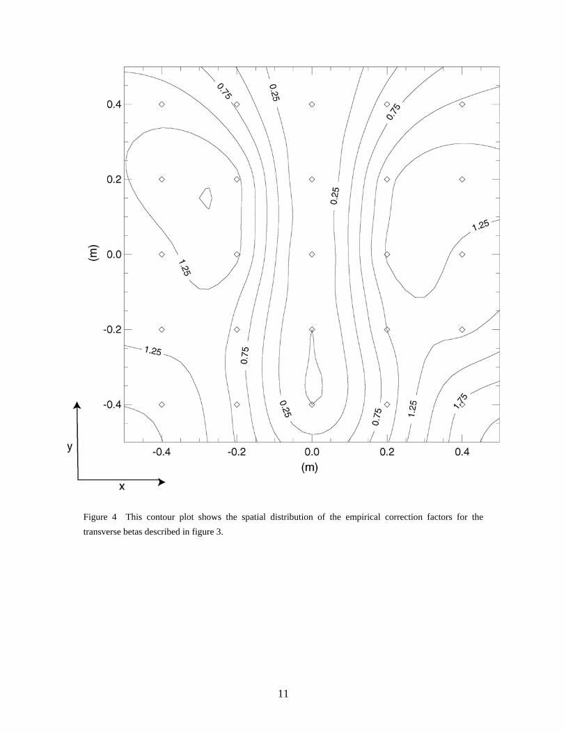
Figure 4 This contour plot shows the spatial distribution of the empirical correction factors for the transverse betas described in figure 3.

11

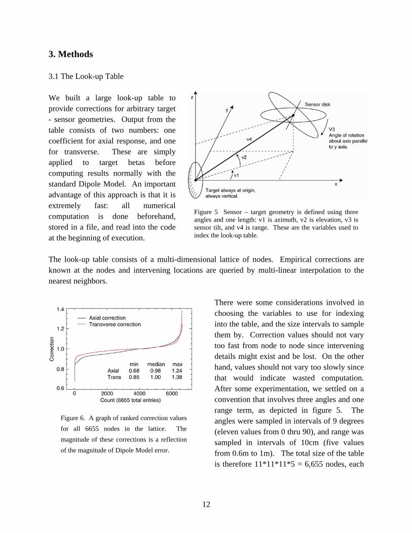
3. Methods 3.1 The Look-up Table We built a large look-up table to provide corrections for arbitrary target - sensor geometries. Output from the table consists of two numbers: one coefficient for axial response, and one for transverse. These are simply applied to target betas before computing results normally with the standard Dipole Model. An important advantage of this approach is that it is extremely fast: all numerical computation is done beforehand, stored in a file, and read into the code at the beginning of execution.

Figure 5 Sensor – target geometry is defined using three angles and one length: v1 is azimuth, v2 is elevation, v3 is sensor tilt, and v4 is range. These are the variables used to index the look-up table.

The look-up table consists of a multi-dimensional lattice of nodes. Empirical corrections are known at the nodes and intervening locations are queried by multi-linear interpolation to the nearest neighbors.

Figure 6. A graph of ranked correction values for all 6655 nodes in the lattice. The magnitude of these corrections is a reflection of the magnitude of Dipole Model error.

There were some considerations involved in choosing the variables to use for indexing into the table, and the size intervals to sample them by. Correction values should not vary too fast from node to node since intervening details might exist and be lost. On the other hand, values should not vary too slowly since that would indicate wasted computation. After some experimentation, we settled on a convention that involves three angles and one range term, as depicted in figure 5. The angles were sampled in intervals of 9 degrees (eleven values from 0 thru 90), and range was sampled in intervals of 10cm (five values from 0.6m to 1m). The total size of the table is therefore 11*11*11*5 = 6,655 nodes, each

12

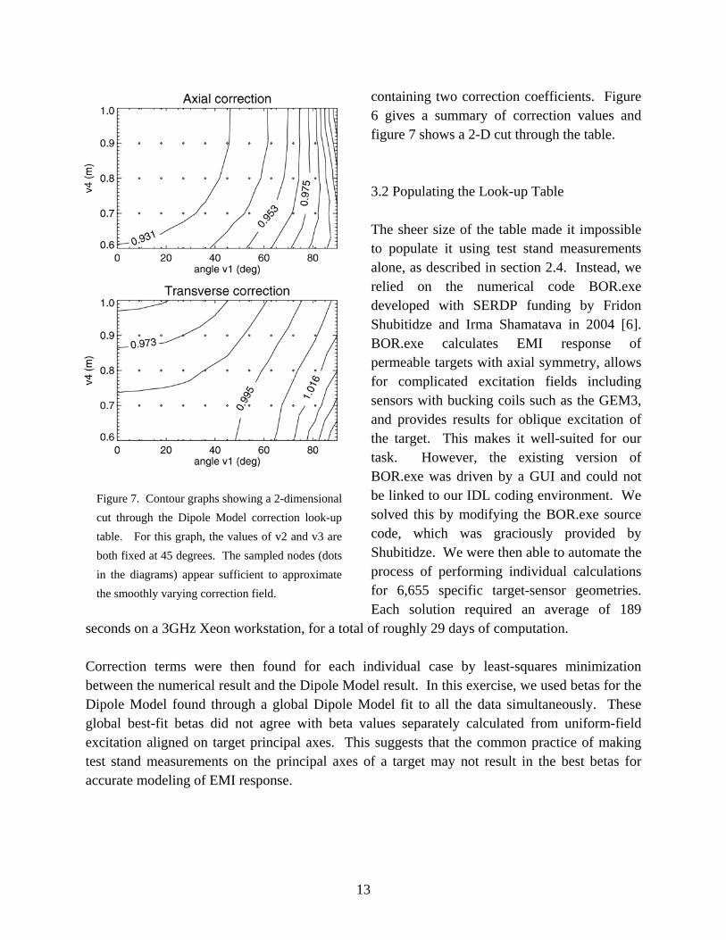
containing two correction coefficients. Figure 6 gives a summary of correction values and figure 7 shows a 2-D cut through the table. 3.2 Populating the Look-up Table The sheer size of the table made it impossible to populate it using test stand measurements alone, as described in section 2.4. Instead, we relied on the numerical code BOR.exe developed with SERDP funding by Fridon Shubitidze and Irma Shamatava in 2004 [6]. BOR.exe calculates EMI response of permeable targets with axial symmetry, allows for complicated excitation fields including sensors with bucking coils such as the GEM3, and provides results for oblique excitation of the target. This makes it well-suited for our task. However, the existing version of BOR.exe was driven by a GUI and could not be linked to our IDL coding environment. We solved this by modifying the BOR.exe source code, which was graciously provided by Shubitidze. We were then able to automate the process of performing individual calculations for 6,655 specific target-sensor geometries. Each solution required an average of 189

seconds on a 3GHz Xeon workstation, for a total of roughly 29 days of computation.

Figure 7. Contour graphs showing a 2-dimensional cut through the Dipole Model correction look-up table. For this graph, the values of v2 and v3 are both fixed at 45 degrees. The sampled nodes (dots in the diagrams) appear sufficient to approximate the smoothly varying correction field.

Correction terms were then found for each individual case by least-squares minimization between the numerical result and the Dipole Model result. In this exercise, we used betas for the Dipole Model found through a global Dipole Model fit to all the data simultaneously. These global best-fit betas did not agree with beta values separately calculated from uniform-field excitation aligned on target principal axes. This suggests that the common practice of making test stand measurements on the principal axes of a target may not result in the best betas for accurate modeling of EMI response.

13

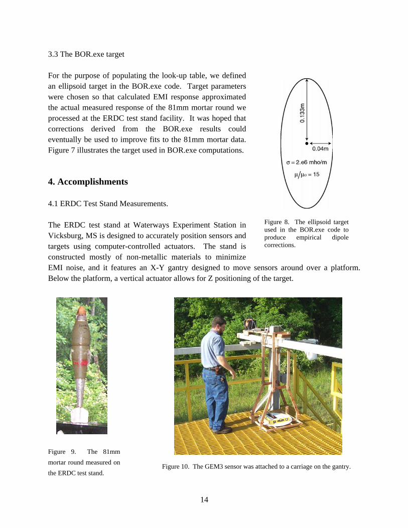
3.3 The BOR.exe target For the purpose of populating the look-up table, we defined an ellipsoid target in the BOR.exe code. Target parameters were chosen so that calculated EMI response approximated the actual measured response of the 81mm mortar round we processed at the ERDC test stand facility. It was hoped that corrections derived from the BOR.exe results could eventually be used to improve fits to the 81mm mortar data. Figure 7 illustrates the target used in BOR.exe computations. 4. Accomplishments 4.1 ERDC Test Stand Measurements. The ERDC test stand at Waterways Experiment Station in Vicksburg, MS is designed to accurately position sensors and targets using computer-controlled actuators. The stand is constructed mostly of non-metallic materials to minimize EMI noise, and it features an X-Y gantry designed to move sensors around over a platform. Below the platform, a vertical actuator allows for Z positioning of the target.

Figure 8. The ellipsoid target used in the BOR.exe code to produce empirical dipole corrections.

Figure 9. The 81mm mortar round measured on the ERDC test stand.

Figure 10. The GEM3 sensor was attached to a carriage on the gantry.

14

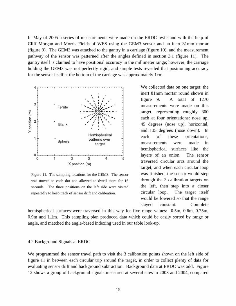
In May of 2005 a series of measurements were made on the ERDC test stand with the help of Cliff Morgan and Morris Fields of WES using the GEM3 sensor and an inert 81mm mortar (figure 9). The GEM3 was attached to the gantry in a carriage (figure 10), and the measurement pathway of the sensor was patterned after the angles defined in section 3.1 (figure 11). The gantry itself is claimed to have positional accuracy in the millimeter range; however, the carriage holding the GEM3 was not perfectly rigid, and simple tests revealed that positioning accuracy for the sensor itself at the bottom of the carriage was approximately 1cm.

We collected data on one target; the inert 81mm mortar round shown in figure 9. A total of 1270 measurements were made on this target, representing roughly 300 each at four orientations: nose up, 45 degrees (nose up), horizontal, and 135 degrees (nose down). In each of these orientations, measurements were made in hemispherical surfaces like the layers of an onion. The sensor traversed circular arcs around the target, and when each circular loop was finished, the sensor would step through the 3 calibration targets on the left, then step into a closer circular loop. The target itself would be lowered so that the range stayed constant. Complete

hemispherical surfaces were traversed in this way for five range values: 0.5m, 0.6m, 0.75m, 0.9m and 1.1m. This sampling plan produced data which could be easily sorted by range or angle, and matched the angle-based indexing used in our table look-up.

Figure 11. The sampling locations for the GEM3. The sensor was moved to each dot and allowed to dwell there for 16 seconds. The three positions on the left side were visited repeatedly to keep track of sensor drift and calibration.

4.2 Background Signals at ERDC We programmed the sensor travel path to visit the 3 calibration points shown on the left side of figure 11 in between each circular trip around the target, in order to collect plenty of data for evaluating sensor drift and background subtraction. Background data at ERDC was odd. Figure 12 shows a group of background signals measured at several sites in 2003 and 2004, compared

15

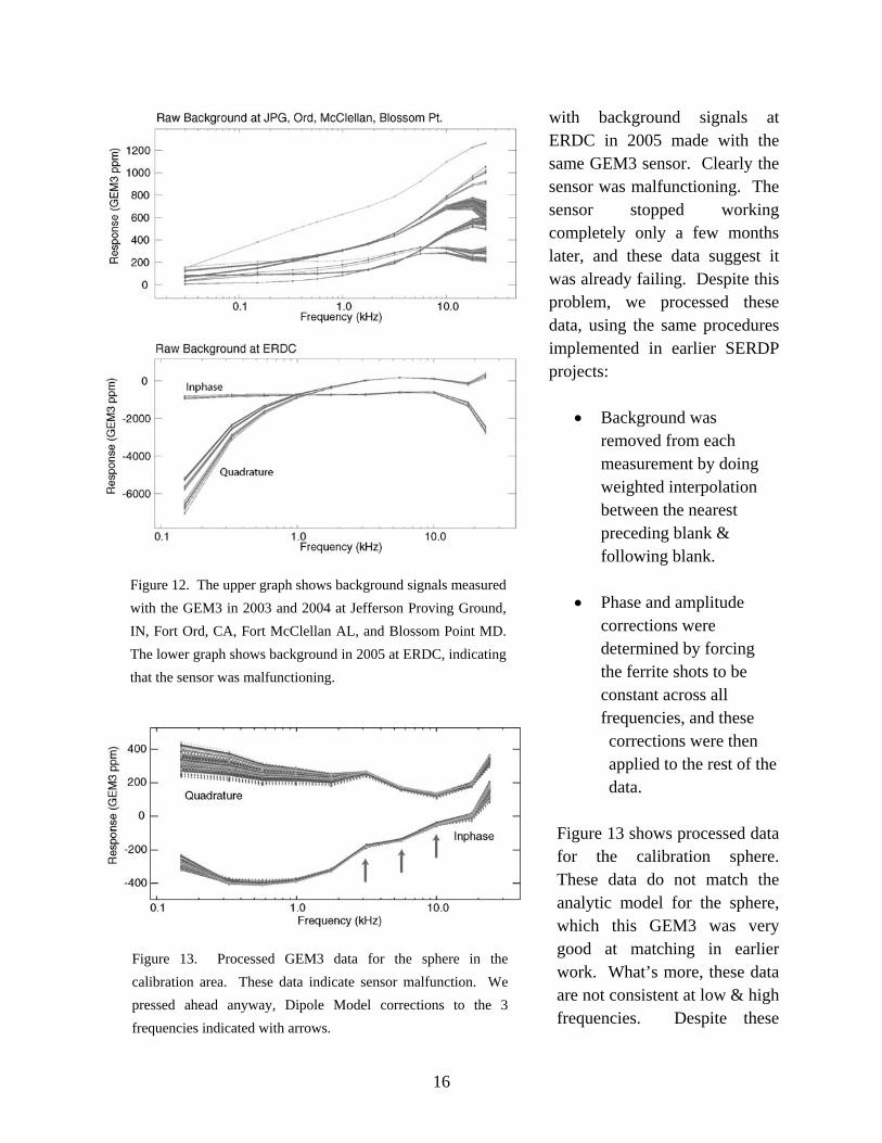
Figure 12. The upper graph shows background signals measured with the GEM3 in 2003 and 2004 at Jefferson Proving Ground, IN, Fort Ord, CA, Fort McClellan AL, and Blossom Point MD. The lower graph shows background in 2005 at ERDC, indicating that the sensor was malfunctioning.

with background signals at ERDC in 2005 made with the same GEM3 sensor. Clearly the sensor was malfunctioning. The sensor stopped working completely only a few months later, and these data suggest it was already failing. Despite this problem, we processed these data, using the same procedures implemented in earlier SERDP projects:

• Background was removed from each measurement by doing weighted interpolation between the nearest preceding blank & following blank.

• Phase and amplitude corrections were determined by forcing the ferrite shots to be constant across all frequencies, and these corrections were then applied to the rest of the data.

Figure 13. Processed GEM3 data for the sphere in the calibration area. These data indicate sensor malfunction. We pressed ahead anyway, Dipole Model corrections to the 3 frequencies indicated with arrows.

Figure 13 shows processed data for the calibration sphere. These data do not match the analytic model for the sphere, which this GEM3 was very good at matching in earlier work. What’s more, these data are not consistent at low & high frequencies. Despite these

16

corruptions, we hoped to salvage something by applying the Dipole Model analysis on the three frequencies shown by the arrows: 3150 Hz, 5610 Hz, and 10050 Hz. 5. Results and Discussion 5.1 Method of evaluation Ideally, data inversion should result in beta values that are fixed for a given target, no matter what particular locations are visited by the sensor. We compared consistency of recovered betas under the usual Dipole Model analysis versus Dipole analysis with empirical corrections. Repeated trials were performed in which random sub-samples of observed data were submitted for beta estimation independently. The spread in recovered values over many trials provides a way to evaluate the usefulness of this empirical Dipole Model correction because beta values are commonly used as inputs for discrimination schemes, and variability contributes to poor performance. Position-referenced EMI data was set up in an IDL environment and random subsets of size 50 were drawn without replacement. Each group of 50 was analyzed twice: once to find best-fit betas using the standard Dipole Model, and a second time using corrections from the look-up table. In both cases, resulting betas were recorded and the process repeated 100 times. 5.2 Evaluation with the ERDC dataset The ERDC data did not produce good results. Figure 14 shows recovered beta values, and there is no evidence of improvement from the Dipole Model correction. As mentioned in the Executive Summary, we speculate that this could be due to corrupt data, since the GEM3 sensor was not working properly, or it could be an indication that Dipole Model corrections have limited applicability across different sensor-target geometries. 5.3 Evaluation with the BOR.exe dataset A synthetic dataset was produced using the same target that was used to create the look-up table (figure 8). These data were then analyzed in the same way the ERDC data was. No noise was added, so any variability in the results must arise because of inherent errors in the Dipole Model, or numerical errors that result from inverting poorly conditioned matrices. As seen in figure 15, the empirical correction produces a marked improvement at all but one frequency. The

17

exception is at 2512Hz Inphase. The reason for this may be that axial inphase beta values are close to zero (figure 16), making it difficult to find best-fit solutions.

Figure 14. Beta estimates from the ERDC dataset for the three frequencies indicated in figure 13. Results from the standard Dipole Model inversion are shown in black, and results from the corrected version are in red. No improvement is seen, possibly because the data was corrupted, or possibly because dipole corrections are not applicable to somewhat different targets.

18

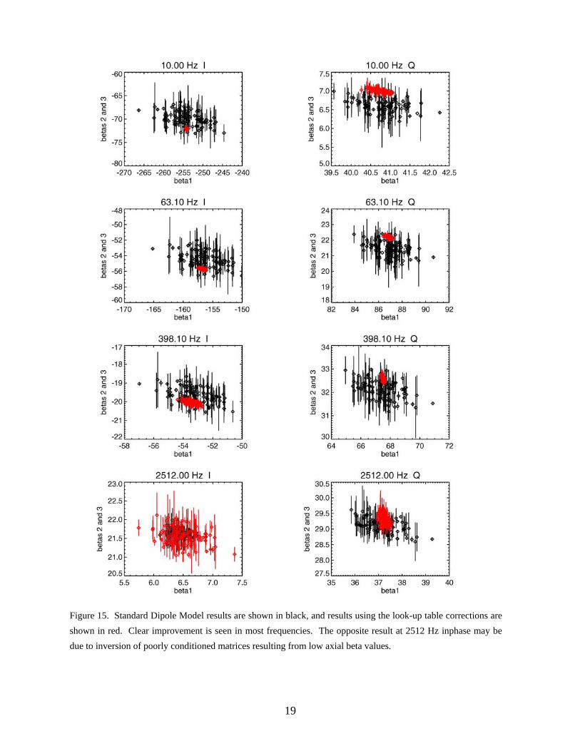
Figure 15. Standard Dipole Model results are shown in black, and results using the look-up table corrections are shown in red. Clear improvement is seen in most frequencies. The opposite result at 2512 Hz inphase may be due to inversion of poorly conditioned matrices resulting from low axial beta values.

19

Figure 16. The beta values used to generate Dipole Model predictions, which were then compared against BOR.exe results to derive empirical corrections. The low inphase axial value at 2512 Hz may be the cause of inversion difficulties.

20

6. References [1] T. Bell, B. Barrow, and J. Miller, “Subsurface Discrimination Using Electromagnetic

Sensors”. IEEE Transactions on Geoscience and Remote Sensing, vol. 39, pp. 1286-1293, June 2001.

[2] N. Geng, C. Baum, and L. Carin, “On the Low-Frequency Natural Response of Conducting and Permeable Targets”, IEEE Trans. Geosci. Remote Sensing, vol. 37, No. 1, pp. 347-359, Jan. 1999.

[3] F. Grant and G. West, 1965, Interpretation theory in applied geophysics: McGraw-Hill Book Co., New York, NY.

[4] S. Ward and G. Hohmann, Electromagnetic Theory for Geophysical Applications, Electromagnetic Methods in Applied Geophysics, Society of Exploration Geophysicists, 1987.

[5] A. Sebak and L. Shafai, “Near-Zone Fields Scattered by Three-Dimensional Highly Conducting Permeable Objects in the Field of an Arbitrary Loop”, IEEE Trans. Geosci. Remote Sensing, vol. 29, No. 1, pp. 9-15, Jan. 1991.

[6] Shamatava, K. O’Neill, Fridon Shubitidze, Keli Sun, Keith D. Paulsen. “Treatment of a permeable non-conducting medium with the EMI-BOR program”. Proc. SPIE Vol. 5794 p. 287-295, Detection and Remediation Technologies for Mines and Minelike Targets X; Russell S. Harmon, J. Thomas Broach, John H. Holloway, Jr.; Eds.

21