Empirical Bayes vs. fully Bayes variable selectionedgeorge/Research... · George and Foster s EB...

Author's personal copy

Journal of Statistical Planning and Inference 138 (2008) 888– 900www.elsevier.com/locate/jspi

Empirical Bayes vs. fully Bayes variable selection

Wen Cuia,∗, Edward I. Georgeb

aTexas State University, San Marcos, TX 78666, USAbThe Wharton School, 3730 Walnut Street, 400 JMHH, Philadelphia, PA 19104-6340, USA

Received 30 December 2004; accepted 28 February 2007Available online 25 April 2007

Abstract

For the problem of variable selection for the normal linear model, fixed penalty selection criteria such as AIC, Cp , BIC andRIC correspond to the posterior modes of a hierarchical Bayes model for various fixed hyperparameter settings. Adaptive selectioncriteria obtained by empirical Bayes estimation of the hyperparameters have been shown by George and Foster [2000. Calibration andEmpirical Bayes variable selection. Biometrika 87(4), 731–747] to improve on these fixed selection criteria. In this paper, we studythe potential of alternative fully Bayes methods, which instead margin out the hyperparameters with respect to prior distributions.Several structured prior formulations are considered for which fully Bayes selection and estimation methods are obtained. Analyticaland simulation comparisons with empirical Bayes counterparts are studied.© 2007 Elsevier B.V. All rights reserved.

Keywords: Hyperparameter uncertainty; Model selection; Objective Bayes

1. Introduction

We consider the variable selection problem in the context of normal linear regression. Suppose the relationshipbetween a dependent variable, Y, and potential explanatory variables, X1, . . . , Xp, can be described by a normal linearmodel,

Y = X� + �, (1)

where Y is n × 1, X is n × p, and � ∼ Nn(0, �2I ). The variable selection problem arises when there is uncertaintyabout which, if any, of the explanatory variables should be dropped from the model. Letting � = 1, . . . , 2p index thesubsets of X1, . . . , Xp, and letting X� be the n × q� design matrix corresponding to the �th subset, this corresponds touncertainty about which is the appropriate subset model

Y = X�� + �. (2)

A common strategy under such variable selection uncertainty has been to select the �th model which maximizes apenalized regression sum of squares criterion of the form

SS�/�2 − F − q�. (3)

∗ Corresponding author. Tel.: +1 512 245 3237; fax: +1 512 245 1452.E-mail addresses: [email protected] (W. Cui), [email protected] (E.I. George).

0378-3758/$ - see front matter © 2007 Elsevier B.V. All rights reserved.doi:10.1016/j.jspi.2007.02.011


W. Cui, E.I. George / Journal of Statistical Planning and Inference 138 (2008) 888–900 889

Here SS� = �LS� X′

�X��LS� is the regression sum of squares of the �th model, where �LS

� is the conditional least squares

estimate of ��, �2 is an estimate of �2 (such as the classical unbiased estimate based on the full model) and F is a fixedpenalty for adding a variable. Such criteria include AIC (Akaike, 1973) and Cp (Mallows, 1973) when F = 2; BIC(Schwarz, 1978) when F = log n; and RIC (Foster and George, 1994) when F = 2 log p.

More recently, a wide variety of semiautomatic and objective Bayesian approaches to the variable selection problemhave appeared in the literature, for example, see Berger and Pericchi (2001), Chipman et al. (2001), Clyde and George(2004), Casella and Moreno (2006) and the references therein. Of particular interest for this paper, are the empiricalBayes (EB) criteria proposed by George and Foster (2000) which were further developed and extended by Clyde andGeorge (2000) and Johnstone and Silverman (2004).

George and Foster’s EB criteria also entail maximization of a penalized sum of squares such as (3) but with Freplaced by adaptive dimensionality penalties that are obtained via a Bayesian calibration to the data. The model forthis calibration uses the hierarchical mixture prior on �� and �,

p(��, � | c, �) = p(�� | �, c)p(� |�), (4)

where

p(�� | �, c) = Nq�(0, c(X′�X�)

−1�2), c > 0, (5)

and

p(� |�) = �q�(1 − �)p−q� , � ∈ [0, 1]. (6)

This prior is determined by two hyperparameters c and �, where c controls the average size of the ��, and � controlsthe average number of nonzero coefficients in the model. Note that increasing c and/or � serves to increase the overall“strength of the signal”.

The connection between the induced hierarchical Bayes model and penalty criteria of the form (3) is revealed by theposterior for �, namely

p(� |Y, c, w) ∝ exp

{c

2(1 + c)[SS�/�

2 − F(c, w)q�]}

, (7)

where

F(c, w) = 1 + c

c

{2 log

1 − w

w+ log(1 + c)

}. (8)

For fixed Y, c and �, p(� |Y, c, w) is increasing in

SS�/�2 − F(c, w)q�, (9)

which is precisely (3) with F = F(c, w). Thus, selecting the highest posterior model under this prior is equivalentto selecting the model maximizing (3) with F = F(c, w). By suitable choices of c and �, the posterior mode can becalibrated to correspond to traditional fixed penalty criteria such as AIC/Cp, BIC or RIC, respectively.

Rather than using fixed prespecified values for c and �, George and Foster (2000) considered estimating themfrom the data via empirical Bayes. For this purpose, they proposed two approaches, marginal maximum likelihood(MML) and conditional maximum likelihood (CML). MML entails finding c and � that maximize the overall marginallikelihood

L(c, w |Y ) ∝∑�

p(� |w)p(Y | �, c)

∝∑�

wq�(1 − w)p−q�(1 + c)−q�/2 exp

{cSS�

2�2(1 + c)

}, (10)

and inserting them into (9) to obtain

CMML = SS�/�2 − F(c, w)q�. (11)


890 W. Cui, E.I. George / Journal of Statistical Planning and Inference 138 (2008) 888–900

Note that the penalty F(c, w) adapts to the data through the estimates of c and w. George and Foster (2000) showed viasimulations that, as opposed to fixed penalty criteria, the performance of CMML is nearly as good as the best possiblefixed penalty criterion over a broad range of model specifications.

A drawback of CMML is that it can be computationally overwhelming especially when X is nonorthogonal becausemaximizing (10) involves averaging � over the whole model space. To mitigate this difficulty George and Foster (2000)also proposed CCML, an easily computable alternative. CCML entails choosing the model � for which the conditionallikelihood

L∗(c, w, � |Y ) ∝ p(� |w)p(Y | �, c)∝ wq�(1 − w)p−q�(1 + c)−q�/2 exp

{cSS�

2�2(1 + c)

}(12)

is maximized over c, � and �. We further discuss the form of CCML in Section 2.3. Although its performance was notquite as good as that of CMML, George and Foster (2000) showed that CCML offered similar adaptive improvementsover fixed penalty criteria.

The main thrust of this paper is to propose and explore the potential of some fully Bayes (FB) alternatives to theseEB criteria. As opposed to EB estimation of c and �, FB approaches put hyperpriors on c and � and then integratethem out to obtain the marginal posterior, �(� |Y ) over the model space. As with CMML and CCML, the FB posteriormode can then be used for model selection.

For particular conjugate hyperpriors, we obtain nearly closed, easily computable forms for these posteriors whichwe then use for analytical and performance comparisons with CMML and CCML. Because in many statistical decisionproblems, the admissible estimators are either Bayes or limits of Bayes procedures (Berger, 1985), one might anticipatethat such FB procedures would improve over CMML and CCML which are neither Bayes nor limits of Bayes procedures.Surprisingly, it appears that our FB procedures are inferior to CMML and essentially comparable to CCML.

Throughout this paper we condition on � and treat it as if it were known. We do this because eliminating this sourceof uncertainty allows us to more clearly compare the EB and FB procedures both analytically and in terms of theirsimulated performance, which is our main thrust. In practice, of course, it is necessary and important to treat unknown�. As we discuss in Section 4, this can be done for the EB and FB procedures by using plug-in estimates of �. However,a further potential advantage of the FB approach is that it also straightforwardly allows for a Bayesian treatment ofunknown �. Such practical fully Bayesian approaches are considered and studied in Liang et al. (2006).

The structure of this paper is as follows. In Section 2, various priors for c and � are discussed and considered;under the priors, the FB selection criterion is derived and compared with the corresponding EB criteria; FB conditionalposterior mean estimates of � are obtained for inference after selection. In Section 3, the performance of the variousprocedures are compared via simulations. In Section 4, we conclude with a discussion of our findings.

2. Fully Bayes selection criteria

The formulation of an FB selection procedure is straightforward in principle: hyperpriors are chosen for c and w andthen these two hyperparameters are integrated out. FB selection then simply entails selecting the model with highestposterior probability. We begin with a discussion of the choice of the hyperpriors.

2.1. Hyperpriors on � and c

In seeking hyperpriors for c and w, several characteristics are especially desirable. First of all, because we areultimately considering a Bayesian model selection problem, it is crucial to use proper hyperpriors. This avoids theproblem of arbitrary norming constants that would render Bayes factors meaningless. Secondly, because of the typicallylarge number of models in variable selection problems, it is advantageous to have hyperpriors leading to computationallytractable posteriors. In particular, hyperpriors that lead to closed form posterior expressions are ideal. Finally, becausevery little, if any, subjective prior information is available in model selection settings such as ours, it is especiallyappealing to have objective prior formulations that can serve as default settings for automatic use. To satisfy all threeof these desiderata, we turn to conjugate hyperpriors. These are proper, they yield closed form posteriors, and allowfor some reasonable default settings.



We begin with the simple conjugate prior family for w, namely the Beta(wa, wb) distributions, which yields

�wa,wb(�) = �(q� + wa)�(p − q� + wb)

�(p + wa + wb)

�(wa + wb)

�(wa)�(wb). (13)

With mean wa/(wa+wb) and variance decreasing in wa and wb, the hyperparameters wa and wb can be chosen to reflecta preference towards particular models. For example, wa/(wa +wb) small would reflect a preference for parsimoniousmodels. For a default choice, three natural contenders are wa = wb = 1 which yields the uniform hyperprior on w,wa = wb = − 1

2 which yields the Jeffreys prior, and wa = wb = −1 which yields the Haldane prior. For a discussion ofthe relative virtues of these three priors, see Geisser (1984), who preferred wa = wb = 1, and the references therein.

As the default of �wa,wb, we consider wa = wb = 1, which yields

�1,1(�) = 1

p + 1

(p

q�

)−1

, (14)

a special case of a form proposed by George and McCulloch (1993). Note that under (14), the prior on model size

�1,1(q�) = 1

p + 1(15)

is uniform. This stands in stark contrast to the popular uniform prior on �,

�U(�) ≡ 1

2p(16)

which induces the prior on model size

�U(q�) = 1

2p

(p

q�

). (17)

Compared to �U , �1,1 places much more weight on the sparse and the saturated models. Note that �U is the limitingdistribution of �wa,wb

as wa = wb → ∞.Turning to c, we note that (1+c) serves as a scale parameter in the marginal distribution of f (y | c, �). Thus, a natural

choice is the incomplete Inverse Gamma (, b) conjugate form for (1 + c) for c ∈ (0, ∞). This yields the hyperpriorfor c

�,b(c) = M(1 + c)−(1+) exp

{− b

1 + c

}, (18)

where M = b(∫ b

0 t−1e−tdt)−1 and c ∈ (0, ∞). As will be seen in Section 2.2, this prior leads to nearly closed formposterior expressions involving only a single one dimension integral.

The prior in (18) is controlled by two hyperparameters, and b that control its shape and scale. As and b areincreased the prior becomes less flat and more concentrated near 0. Thus, in the spirit of stable estimation, a naturaldefault choice would entail using small values for and b. For this purpose, we recommend setting b = 0 and using

�(c) = (1 + c)−(1+) for c ∈ (0, ∞) (19)

with = 1 as the default prior on c. Although even smaller choices for might be considered, extensive simulationstudies in Cui (2002) suggest that the performance of the FB procedures, which we discuss below, is robust to smallchanges around = 1. It might be noted that = 0 and b = 0 yields an improper prior which is proportional to theJeffrey’s prior conditional on �. Because it is not proper, such a prior does not appear to be useful for model selection.

Priors of the form (19) were also recently and independently proposed for the variable selection problem by Lianget al. (2006). Referring to them as hyper-g priors, they studied these for the important practical case of unknownvariance in conjunction with �(�2) ∝ 1/�2. Priors of the form (19) were also proposed by Strawderman (1971) for thesomewhat different context of minimax estimation of a multivariate normal mean with identity covariance.

As an alternative to priors of the form (18), one might instead consider Inverse Gamma hyperpriors on c ratherthan on (1 + c). Such a conjugate choice is implicit in the work of Zellner and Siow(1980); Zellner and Siow (1984).



Motivated by Jeffreys (1967), Zellner and Siow proposed testing H1 : �� = 0 versus H2 : �� = 0 using multivariateCauchy priors with covariance X′

�X�/n for �(�� |�) and �(�) ∝ 1/�2. Such priors would be obtained here by putting

an inverse Gamma hyperprior IG( 12 , n/2) directly on c. Unfortunately, posteriors under this prior are computationally

more difficult to approximate than posteriors under (19). Zellner–Siow priors for variable selection with unknown �were also extensively studied by Liang et al. (2006).

2.2. Fully Bayes posteriors

Under the Beta(wa, wb) hyperprior for w and the incomplete gamma conjugate form (18) for c, the Normal–Bernoullisetup (5)–(6), and the linear model (1), the model posterior is straightforwardly obtained as

�(� |Y ) = K · M exp

{SS�

2�2

}(b + SS�

2�2

)−q�/2−

G,b(SS�, q�)�wa,wb(�) (20)

for q� = 0 and

�(� |Y ) = K · �wa,wb(�) (21)

for q� = 0, where

K = (2�)−n/2(�2)−n/2 exp

{−Y ′Y

2�2

}/m(Y), (22)

G,b(SS�, q�) =∫ SS�/2�2+b

0tq�/2+−1e−t dt , (23)

m(Y) is the overall marginal density function of Y, and M is the norming constant in (18).For our default prior choices �1,1(�) in (14) and �1(c) in (19), the model posterior reduces to

�(� |Y ) = K exp

{SS�

2�2

}(SS�

2�2

)−q�/2−1

G(SS�, q�)�1,1(�) (24)

for q� = 0 and

�(� |Y ) = K

p + 1(25)

for q� = 0, where

G(SS�, q�) =∫ SS�/2�2

0tq�/2e−t dt . (26)

Model selection under any one of these posteriors can then simply proceed by choosing the model � that maximizes�(� |Y ). For comparisons with empirical Bayes criteria, we focus on the default fully Bayes criterion obtained bymaximizing (24) and (25).

2.3. Comparison of CFB and CCML

It is interesting to compare the default fully Bayes criterion that maximizes (24) with the empirical Bayes criterionthat maximizes (12). To do this, we consider the penalized sum of squares representation of the empirical Bayes criterion

CCML ={

SS�/�2 − B(SS�, q�) − R(q�) if q� = 0,

0 if q� = 0,(27)

where letting I� = 1 if SS�/�2q� > 1 and I� = 0 otherwise,

B(SS�, q�) = I�q�

{1 + log

(SS�

�2q�

)}+ (1 − I�)

SS�

�2 (28)



and

R(q�) = −2{(p − q�) log(p − q�) + q� log q�}. (29)

As shown by George and Foster (2000), the component B is a consequence from estimating c and acts like BIC, whereasthe component R is a consequence from estimating � and acts like RIC. (The expression for CCML above corrects aminor error in the expression for CCML in George and Foster (2000). However, the error is relatively unimportant as itoccurs only when I� = 0, an event of low probability).

By maximizing 2 log �(� |Y ) with irrelevant constants removed, we can express the default fully Bayes criterion asan analogous penalized sum of squares criterion, denoted by CFB,

CFB ={

SS�/�2 − B∗(SS�, q�) − R∗(q�) if q� = 0,

0 if q� = 0,(30)

where

B∗(SS�, q�) = (q� + 2) logSS�

2�2 − 2 log G(SS�, q�) (31)

and

R∗(q�) = −2{log(p − q�)! + log q�! − log(p + 1)!}. (32)

Analogous to the CCML penalties B and R, here B∗ and R∗ are the penalties due to marginalizing over c and w,respectively.

It is interesting to compare the respective penalties of CCML and CFB when the model dimension goes from q� − 1to q� with a negligible change in SS�, corresponding to the addition of an unimportant variable. Assuming no changein SS� and that SS�/�2q� > 1, the change in B is obtained as

�B(SS�, q�) =(

1 + logSS�

�2q�

)− (q� − 1) log

q�

q� − 1. (33)

Under the same assumptions, the change in B∗ is

�B∗(SS�, q�) = logSS�

2�2 − 2 logG(SS�, q�)

G(SS�, q� − 1)(34)

≈ logSS�

2�2 − 2 log(SS�/2�2)(q�/2)q�/2e−q�/2

(SS�/2�2)((q� − 1)/2)(q�−1)/2e−(q�−1)/2(35)

=(

1 + logSS�

�2q�

)− (q� − 1) log

q�

q� − 1, (36)

where we have used the upper bound approximation

G(SS�, x) =∫ SS�/2�2

0tx/2e−t dt ≈ SS�

2�2

(x

2

)x/2e−x/2 (37)

(txe−t is maximized at t =x). Note that when SS�/�2q� > 1, q�/2 is within the range of integration, thereby improvingthe quality of this approximation.

Turning to the relative changes in R and R∗, George and Foster (2000) use the approximation

1 + log q ≈ q log q − (q − 1) log(q − 1) (38)



to show that

�R(q�) ≈ 2 logp − q� + 1

q�. (39)

For the CFB criterion, this approximation turns out to be exact

�R∗(q�) = 2 logp − q� + 1

q�. (40)

Thus, we see that, at least for small changes in SS�, the penalties imposed by CCML and CFB are very similar.

2.4. Estimation of �� after selection

When CFB is used to select a model �, it will usually also be of interest to estimate the corresponding vector ofcoefficients ��. For this purpose in the fully Bayes framework, it is most natural to use the conditional posterior meanof �� given the selected �, namely E(�� |Y, �). Under our default priors, an easily computable expression for this isobtained as

�FB� = E(�� | �LS

� , �) =(

1 − 2�2

SS�

G(SS�, q� + 2)

G(SS�, q�)

)�LS

� , (41)

where �LS� is the conditional least squares estimate of ��. This follows using E(�� |Y, �) = E(E(�� | �LS

� , �, c)) and

the fact that E(�� | �LS� , �, c) = (c/(1 + c)) �LS

� under the normal prior (5).In contrast, in the empirical Bayes framework, one further conditions on the estimate c. For CMML, this yields

�MML� = E(�� |Y, �, c) = c

1 + c�LS

� , (42)

where c is the maximum marginal likelihood estimate of c. Although this can be numerically computed, no closed formrepresentation for �MML

� is available. However, for CCML, the EB posterior mean is obtained in closed form as

��CML =

(1 − �2q�

SS�

)+�LS

� , (43)

where (a)+ denotes the positive part of a. The approximation

��FB ≈

(1 − �2(q� + 2)

SS�

)+�LS

� , (44)

which is obtained from (41) using (37) and then (38), reveals that �CML� and �FB

� are very similar. Note that all three of

these posterior mean estimators shrink �LS� towards zero.

3. Simulation evaluations

We now turn to simulation comparisons of our default fully Bayes procedures CFB with the empirical Bayes pro-cedures CMML and CCML. To shed light on the effect of the model space prior �1,1(�) in (14), we have included thedefault fully Bayes procedure which, like CFB, uses �1(c) in (19) but replaces �1,1(�) by the uniform �U(�) in (16).The resulting criterion to be maximized, which we denote CFBU, differs from CFB in (30) only in that R∗(q�) in(32) is replaced by a constant. Finally, for added perspective we also included AIC and BIC, the traditional penalizessum-of-squares criteria with fixed penalties F = 2 and F = log n, respectively.

From a decision theoretic point of view, the appropriate loss for such selection rules is the 0–1 loss function whichis 0 if and only if the correct model is selected. However, using such a loss function for simulation is problematicbecause getting the model exactly right is a very small probability event when so many models are being compared.



0 500 1000

0

Ma

xim

um

lo

g p

oste

rio

rsThe actual model is the null model

0 500 1000

0

100

log

po

ste

rio

rs

The actual model size is 50

0 500 1000

0

100

200

log

po

ste

rio

rs


0 500 1000

0

200

400

600

800

Ma

xim

um

lo

g p

oste

rio

rs


0 500 1000

0

200

400

600

800

1000

1200

log

po

ste

rio

r


0 500 1000

0

500

1000

1500

log

po

ste

rio

rs

The actual model is the full mode

-100

-200

-300

-400

-500

-600

-100

-200

-300

-400

-500

-100

-200

-300

-400

-500

-600

-700

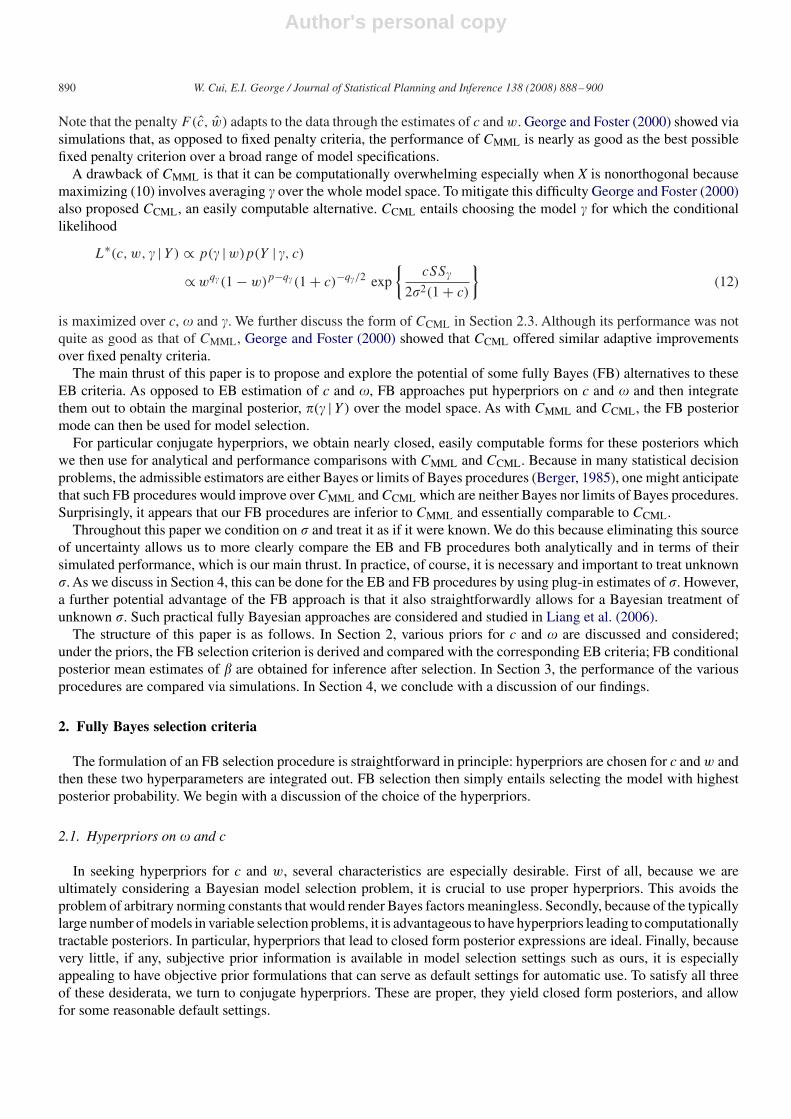
Fig. 1. FB maximum log posteriors.

Furthermore, such a loss function ignores the extent to which the selected model differs from the correct model; gettingmost of the variables correct is not rewarded at all.

Thus, as in George and Foster (2000), we find it more informative to summarize the performance of the variousselection rules by the predictive error loss

L{�, ��} ≡ {X�� − X�}′{X�� − X�}, (45)

where �� is an estimator of �� conditionally on the selected �. For the purpose of comparing the selection criteria CMML,

CCML, CFB, CFBU, AIC and BIC, we use �� = �LS� . For the purpose of evaluating and comparing the estimation-after-

selection posterior mean rules, �MML� , �CML

� , �FB� and �FBU

� , we substitute each of these for �� in (45). Note that �FBU�

is obtained just as�FB� in (41) except that � is instead selected using CFBU.

For simplicity, we assume that �2 = 1 is known, and focus exclusively on the orthogonal case where X = I , asetting that arises naturally in nonparametric regression. In this case, the regression model (2) is of the simple formY = � + �. Following George and Foster (2000), we generated data as follows. For n = p = 1000 and fixed values of qand c, we generated the first q components of � as independent N(0, c) realizations, set �q+1 = �q+2 = · · · = �p = 0,independently generated � ∼ Np(0, Ip), and then calculated Y = � + �. This procedure was replicated 1000 timesand the average loss (45) was calculated for each procedure. These average losses were obtained for each value ofq = 0, 10, 25, 50, 100, 300, 500, 700, 900, 1000 when c = 5, 25. Note that c = 5 and c = 25, respectively, correspondto weak and strong signal-to-noise ratios.

We remark that for each fixed q�, the posterior �(� |Y ) in (24), is monotonically increasing in SS�. This propertyallows us to easily identify the highest posterior models when X is orthogonal by simply using greedy forward selectionof Y coordinates to obtain the sequence of maximal SS� values for q = 0, . . . , 1000. If X is nonorthogonal and theproblem is large, one must resort to methods that heuristically restrict attention to a subset of the model space, and thenapply the selection criteria to the subset.

Before proceeding, we should point out a feature that CFB shares with CCML, namely a tendency towards bimodalityover the � space. This is illustrated by the six plots in Fig. 1 which display the maximum of the log posterior (24) foreach model size q over 50 simulations of six of our model setups. Note that for moderate size models, true model sizetends to fall between location of the two nodes. These plots were typical of what we saw in most of the simulations. Insharp contrast, Fig. 2 reveals no bimodality whatsoever in the log posteriors corresponding to CFBU for the identicaldata. This shows quite clearly that the bimodality of CFB is entirely due to effect of the prior �1,1(�) which, as was



0 500 1000

Maxim

um

log p

oste

riors

The actual model is the null model

0 500 1000

log p

oste

riors


0 500 1000

log p

oste

riors


0 500 1000

0

200

400

Maxim

um

log p

oste

riors


0 500 1000

0

200

400

600

800lo

g p

oste

rior


0 500 1000

0

500

1000

1500

log p

oste

riors

The actual model is the full mode

-550

-600

-650

-700

-200

-400

-600

-200

-400

-600

-400

-450

-500

-450

-600

-650

-700

-100

-200

-300

-400

-500

-600

-700

-500

Fig. 2. FBU maximum log posteriors.

Table 1Average losses over 1000 replications of the selection rules MML = CMML, CML = CCML, FB = CFB, FBU = CFBU, AIC and BIC, and of the

posterior mean rules �MML� , �

CML� �

FB� and �

FBU�

q 0 10 25 50 100 300 500 700 900 1000

Average losses when c = 5CMML 3.7 36.7 79.2 144.1 259.5 625.3 878.9 998.0 1000.3 1001.8CCML 0.3 35.1 81.1 149.9 273.6 682.2 990.3 1210.6 1301.9 1170.7CFB 0.3 35.2 81.0 149.3 273.2 681.4 989.7 1209.9 1301.2 1169.6CFBU 633.0 625.5 618.4 614.0 618.4 715.2 864.0 1024.9 1188.7 1274.2AIC 572.6 577.0 586.4 603.7 636.5 755.3 879.1 1002.1 1125.5 1188.1BIC 75.7 93.3 120.6 169.2 261.8 635.9 1008.6 1382.5 1756.7 1943.8

�MML� 1.3 31.8 70.5 127.8 227.7 527.4 714.3 794.3 820.3 834.2

�CML� 0.3 34.7 80.1 147.6 268.1 659.3 944.6 1137.9 1196.4 1029.7

�FB� 0.2 34.7 79.5 146.5 267.1 658.0 943.5 1136.7 1195.2 1028.4

�FBU� 307.2 326.8 353.0 387.9 439.8 594.3 750.6 909.7 1068.7 1150.0

Average losses when c = 25CMML 1.5 35.3 75.1 137.4 240.4 570.8 814.0 964.9 999.9 999.8CCML 0.1 36.1 77.5 141.3 247.6 589.7 844.4 1006.3 1004.5 999.8CFB 0.1 35.6 77.0 141.1 247.1 589.5 844.2 1006.1 1004.6 999.8CFBU 633.2 573.8 514.5 467.0 456.8 610.5 812.3 1013.8 1222.0 1327.7AIC 572.8 578.4 586.3 600.3 628.2 735.9 853.4 963.0 1075.3 1132.9BIC 76.2 91.5 117.4 162.0 246.0 593.8 943.0 1284.2 1629.7 1808.7

�MML� 0.6 34.2 73.0 133.7 233.4 551.0 781.7 923.1 957.9 961.1

�CML� 0.1 35.7 76.5 139.5 243.7 577.3 822.6 976.0 962.6 961.1

�FB� 0.1 35.2 75.9 139.1 243.2 576.9 822.3 975.7 962.8 961.1

�FBU� 307.3 373.9 400.3 404.4 420.7 585.3 785.0 984.0 1189.0 1292.5



0 10 25 50 100

0

200

400

600

800

1000

1200

1400

q

Avera

ge L

osses

Average losses: c = 5 and

q = 0, 10, 25, 50 and 100

MML

CML

FB

FBU

AIC

BIC

300 500 700 900 1000

600

800

1000

1200

1400

1600

1800

q

Avera

ge L

osses


q = 300, 500, 700, 900 and 1000

MML

CML

FB

FBU

AIC

BIC

0 10 25 50 100

0

200

400

600

800

1000

1200

1400

q

Avera

ge L

osses


q = 0, 10, 25, 50 and 100

MML

CML

FB

FBU

AIC

BIC

300 500 700 900 1000

600

800

1000

1200

1400

1600

1800

q

Avera

ge L

osses


q = 300, 500, 700, 900 and 1000

MML

CML

FB

FBU

AIC

BIC

Fig. 3. Average losses over 1000 replications of the selection rules MML = CMML, CML = CCML, FB = CFB, FBU = CFBU, AIC and BIC.

pointed out in Section 2.1, puts much larger weight on the sparse (small q�) and saturated (large q�) models. BecauseCCML is implicitly using approximately this prior, this evidently also explains the posterior bimodality of CCML, ratherthan the speculative bimodality explanation given by George and Foster (2000). To mitigate the bimodality difficultyin practice, we recommend selecting the more parsimonious of the two models when such bimodality is present. Thismodification, also used by George and Foster (2000) for CCML, helped to improve the performance of CFB for smallerq models.

Table 1 presents the average losses over 1000 simulations of the setup described above, for the EB selection rulesCMML, CCML, the FB selection rules CFB, CFBU, the fixed penalty selection rules AIC and BIC, and the estimation-after-selection posterior mean rules �MML

� , �CML� , �FB

� and �FBU� . For visual comparisons, these selection rule losses

are plotted in Fig. 3 and the posterior mean rule losses are plotted in Fig. 4.The main focus of our investigation is the extent to which CFB compares with CMML and CCML. We can see

immediately from Table 1 and Fig. 3 that when c = 5, corresponding to a low signal-to-noise ratio, CMML performedmarkedly better than both CFB and CCML except for very small values of q. When c=25, CMML was still best, althoughby a lesser extent, again except for very small values of q. It is also clear that, just as the analytical comparisons inSection 2.3 suggested, CFB and CCML are essentially equivalent, although CFB seems to perform very slightly betterthan CCML.



0 10 25 50 100

0

200

400

600

800

1000

1200

q

Ave

rage

Los

ses

Average losses: c = 5 andq = 0, 10, 25, 50 and 100

BMMLBCMLBFBBFBU

300 500 700 900 1000

600

800

1000

1200

1400

1600

1800

q

Ave

rage

Los

ses


BMMLBCMLBFBBFBU

0 10 25 50 100

0

200

400

600

800

1000

1200

q

Ave

rage

Los

ses


BMMLBCMLBFBBFBU

300 500 700 900 1000

600

800

1000

1200

1400

1600

1800

q

Ave

rage

Los

ses


BMMLBCMLBFBBFBU

Fig. 4. Average losses over 1000 replications of the posterior mean rules �MML� , �

CML� , �

FB� and �

FBU� .

Turning to CFBU, Table 1 and Fig. 3 reveal that replacing �1,1(�) by the uniform �U(�) has a substantial effect. CFBperformed substantially better than CFBU for smaller q, and for larger q when c=25. Compared to AIC and BIC, whichwe included simply to add perspective, CMML, CCML and CFB are all clearly superior. In particular, AIC is much worsewhen q is small and BIC is much worse when q is large, a reflection of their inability to adapt. Finally, Table 1 and Fig.4 reveal that the estimation-after-selection posterior mean rules, �MML

� , �CML� , �FB

� and �FBU� all uniformly improve on

their least squares counterparts CMML, CCML, CFB and CFBU, especially for c = 5 when the components of � are onaverage smaller and shrinkage is more likely to be effective. Not surprisingly, the relative performance of these fourposterior mean rules parallel exactly the relative performance of their counterparts.

4. Discussion

When we began this research, we were hopeful that we would find a fully Bayes selection procedure that wassuperior to the empirical Bayes procedure. We were surprised to find that CFB was not as good as CMML and wasessentially equivalent to CCML. In retrospect, the explanation for this may be understood by noting that MML estimateof c incorporates information across all potential models, whereas the CML estimate is based on the single maximized



model. Rather than estimate c, the fully Bayes procedure margins out c out of each model separately via

p(� |Y ) ∝ �(�)∫

p(Y | c, �)�(c) dc. (46)

This integration does not incorporate information outside of the �th model, and so behaves like the implicit CMLposterior p(� |Y ) ∝ �(� | w)p(Y | c, �). Thus, the similarity between CFB and CCML was to be expected. Note that theprior �(c) is not the issue here.

The dominance of the MML procedure over the FB procedure persisted in our comparisons of the conditionalposterior mean estimators �FB

� , �MML� and �CML

� . However, in principle, one can go further and consider the Bayes ruleunder squared error loss, namely the unconditional posterior mean of � under the hyperpriors on c and w. This modelaveraged estimator would incorporate information across all the potential models and would likely dominate the EBcounterparts. Unfortunately, when p is large, such an estimate will be prohibitively expensive to calculate. However, aninteresting and computable hybrid alternative proposed by Johnstone and Silverman (2004) integrates out c with respectto a prior, but then uses an empirical Bayes estimate of the median w. Insofar as the posterior median approximatesthe posterior mean, this estimator is a promising EB alternative.

In this paper, we have focused on the orthogonal case which simplifies the computation of both the EB and FBprocedures. However, when X is nonorthogonal, MML calculations will no longer be feasible even in moderately sizedproblems, and so CMML must be ruled out. Although CCML and CFB can still be pursued, it should be noted that findingthe posterior mode will no longer be practical in large problems where it is not feasible to evaluate the posteriors ofall the 2p models. In such cases, heuristics such as stepwise methods or stochastic search might be used to restrictattention to a manageable set of models.

Finally, as mentioned in Section 1, we have considered only the case where �2 is known in order to focus on the contrastbetween the EB and FB approaches to hyperparameter uncertainty. However, the more realistic and practical case ofunknown �2 can be addressed in all these procedures. A straightforward approach for the EB and FB procedures is to set�2 equal to a plug-in estimate such as the traditional full model estimate (Y ′Y −SSp)/(n−p) or, in the nonparametric

regression case where n=p, to use the robust median estimate �=median(|�i |)/0.6745 (Donoho et al., 1995). But forFB procedures, one can do even better by integrating out �2 with respect to a prior such as �(�2) ∝ 1/�2 as in Zellnerand Siow(1980); Zellner and Siow (1984) and Liang et al. (2006).

Acknowledgments

We would like to thank the editor, two anonymous referees and Merlise Clyde for helpful comments and suggestions.This work was supported by a number of NSF Grants, where DMS-0605102 is the most recent.

References

Akaike, H., 1973. Information theory and an extension of the maximum likelihood principle. In: Petrov, B.N., Csaki, F. (Eds.), Second InternationalSymposium on Information Theory. Akademia Kiado, Budapest, pp. 267–281.

Berger, J.O., 1985. Statistical Decision Theory and Bayesian Analysis. Springer, New York.Berger, J.O., Pericchi, L., 2001. Objective Bayesian methods for model selection: introduction and comparison. In: P. Lahiri (Ed.), Model Selection.

IMS Lecture Notes—Monograph Series, vol. 38. Institute of Mathematical Statistics, pp. 135–193.Casella, G., Moreno, E., 2006. Objective Bayesian variable selection. J. Amer. Statist. Assoc. 101, 157–167.Chipman, H., George, E.I., McCulloch, R.E., 2001. The practical implementation of Bayesian model selection. In: P. Lahiri (Ed.), Model Selection.

IMS Lecture Notes—Monograph Series, vol. 38. Institute of Mathematical Statistics, pp. 65–134.Clyde, M., George, E.I., 2000. Flexible empirical Bayes estimation for wavelets. J. Roy. Statist. Soc. Ser. B 62, 681–698.Clyde, M., George, E.I., 2004. Model uncertainty. Statist. Sci. 19 (1), 81–94.Cui, W., 2002. Variable selection: empirical Bayes vs. fully Bayes. Ph.D. Dissertation, Department of MSIS, University of Texas at Austin.Donoho, D., Johnstone, I., Kerkyacharian, G., Picard, D., 1995. Wavelet shrinkage: asymptopia? J. Roy. Statist. Soc. Ser. B 57, 301–369.Foster, D.P., George, E.I., 1994. The risk inflation criterion for multiple regression. Ann. Statist. 22, 1947–1975.Geisser, S., 1984. On prior distribution for binary trials. Amer. Statist. 38 (4), 244–251 (with discussion).George, E.I., Foster, D.P., 2000. Calibration and Empirical Bayes variable selection. Biometrika 87 (4), 731–747.George, E.I., McCulloch, R.E., 1993. Variable selection via Gibbs sampling. J. Amer. Statist. Assoc. 88, 881–889.Jeffreys, 1967. Theory of Probability. Oxford University Press, Oxford.Johnstone, I.M., Silverman, B.W., 2004. Needles and straw in haystacks: Empirical Bayes estimates of possibly sparse sequences. Ann. Statist. 32,

1594–1649.



Liang, F., Paulo, R., Molina, G., Clyde, M.A., Berger, J.O., 2006. Mixtures of g-priors for Bayesian variable selection, ISDS Discussion Paper 05–12.Duke University, Durham, NC.

Mallows, C.L., 1973. Some Comments on Cp . Technometrics 15, 661–676.Schwarz, G., 1978. Estimating the dimension of a model. Ann. Statist. 6, 461–464.Strawderman, W.E., 1971. Proper Bayes minimax estimators of the multivariate normal mean. Ann. of Math. Statist. 42, 385–388.Zellner, A., Siow, A., 1980. Posterior odds ratio for selected regression hypotheses. In: Bernardo, J.M., DeGroot, M.H., Lindley, D.V., Smith, A.F.M.

(Eds.), Bayesian Statistics, vol. 1. University Press, Valencia.Zellner, A., Siow, A., 1984. Basic Issues in Econometrics. University of Chicago Press, Chicago.

Empirical Bayes vs. fully Bayes variable selectionedgeorge/Research... · George and Foster s EB...

Documents

Transcript of Empirical Bayes vs. fully Bayes variable selectionedgeorge/Research... · George and Foster s EB...